Aug 1, 2016 - classes using Random Forest[3], ship detection[2][4], oil slick characterization[5], crop monitoring of rice in China[6] and identification of potato ...
Supervised Classification of RADARSAT-2 Polarimetric Data for Different Land Features
arXiv:1608.00501v1 [cs.CV] 1 Aug 2016
Abhishek Maity Abstract—The pixel percentage belonging to the user defined area that are assigned to cluster in a confusion matrix for RADARSAT-2 over Vancouver area has been analysed for classification. In this study, supervised Wishart and Support Vector Machine (SVM) classifiers over RADARSAT-2 (RS2) fine quadpol mode Single Look Complex (SLC) product data is computed and compared. In comparison with conventional single channel or dual channel polarization, RADARSAT-2 is fully polarimetric, making it to offer better land feature contrast for classification operation. Index Terms—Wishart, Support Vector Machine (SVM), Confusion matrix
I. I NTRODUCTION SAR data analysis for a range of applications from compact and fully Polarimetric SAR like RADARSAT-2 are becoming popular everyday on the fact that they offer features like higher resolution imaging, wide swath, reduced PRFs. Data from these family of SAR are very useful in several applications involving terrain to oceans which are clearly depicted in[1]. The polarimetric data analysis from Convair-580 and RADARSAT2 have resulted many successful studies in fields ranging from ship-detection[2] , land-use pattern, crop classification. With the launch of RADARSAT-2 on December 14, 2007, it became possible to have a SAR system having modes of multiple polarization including full polarimetry and resolution upto 1 metre in spotlight mode. The satellite carries a C-band SAR. In this paper, confusion matrix analysis of RADARSAT2 data has been examined for various feature classification. Many studies have been undertaken for classification using RADARSAT-2 till date. They include classification of terrain classes using Random Forest[3], ship detection[2][4], oil slick characterization[5], crop monitoring of rice in China[6] and identification of potato and rice fields using RADARSAT1 in India[7].Even work like ice-monitoring[8] and mapping of seasonal floods in wetland forests of Brazil has yielded promising results[9]. Research on classification using multitemporal data sets of RADARSAT-2 is also being carried out using different classification algorithms coupled with various functions. II. VANCOUVER STUDY SITE : RS2 DATA Here for the study, we utilize the data set consisting the Greater Vancouver area, Canada. The test site is very diverse in nature consisting a wide variety of features to classify. The area consists of urban settlements including Richmond area, rotated urban areas west to New Westminster. Rugged
Fig. 1. (a) PauliRGB and classification based on supervised (b) SVM (c) Wishart classifiers
mountains in northern Vancouver, rivers merging to the Strait of Georgia and crop-lands in the Fraser River Delta. RADARSAT-2 data has been acquired on May 2008 over Vancouver area in full polarimetric mode. Ground-truth parameters was also collected synchronous with the satellite pass. Near Range Incidence Angle is 34.49o and Far Range Incidence Angle is 36.08o .The dataset of RADARSAT-2 was acquired in Fine Quad mode with Q15 beam. It has been captured in descending pass direction inferring the snap is recorded on the sunlit side as the orbit of the SAR system is sun-synchronous III. M ETHODOLOGY The coherency matrix T of 3 × 3 is generated. Beside T3 matrix, additional polarimetric information like H/A/α coefficients for Target decomposition are computed for performing classification based on Wishart distribution [10]. Speckle is a kind of noise that appears in data obtained through SAR systems. Speckle reduces with multi-looking images. Therefore, we have applied a 3 × 3 look using Lee filter to remove noise keeping loss of information minimum. The coherency matrix T is computed through a scattering vector in the base of Pauli that demonstrate geometrical properties.The equation is given by and is in accordance to [12] SHH + SV V 1 kp = √ SHH − SV V 2 2S HV
[T ] = kp .kp∗T After decomposition from [12] the H entropy shows the wave polarization, where as A or Anisotropy is a difference between the second and third eigenvalue especially significant for the range 0.7 < entropy < 0.9. The α parameter is an important component because it gives the wave reflection mechanisms over the considered pixels. It characterizes the single bound, double bound and volume scattering. A. Wishart Classification The T matrix elements especially dedicated to SAR data involves the Wishart classification as because the presence of speckle noise in the data set account for the Wishart distribution. The polarimetric information for mono-static case is define by the target vector h √SHH h = 2.SHV SV V
Fig. 2. Linear SVM classifier
In the multi-look data that is 3 × 3 case we represent the data by a polarimetric covariance matrix Z n
Z=
1 X . hk h∗T k n k=1
Where hk is nothing but kth sample of h, the superscript * in the equation denote the complex conjugate where as the number of looks (samples) is given by n. As per Wishart distribution the covariance matrix could be expressed as : P−1 Z) nqn |Z|n−q exp−tr(n P n p(Z) = K(n, q)| | with K(n, q) = π
q(q−1)/2
.
q Y
Fig. 3. Non-linear SVM classifier
f (x) = sign(hω, Xi + b) Γ(n − i + 1)
i=1
Where Γ() represents the gamma function and tr() is the trace of the given matrix. The q denotes the number of elements of the obtained target vector h (It is generally 3 for mono-static and 4 for the bi-static). Lastly, the n represent the number of looks. It is to be noted that the Wishart classification consist in a maximum likelihood classification based on a Wishart distribution. B. SVM classification The Support Vector Machine (SVM) are models of supervised learning that basically analyse data used for classification and regression analysis. The work here coincide with [11] and [13]. Linear case: With N training samples, the case of two classes problem is considered. Every sample is described by a Support Vector Xi consisting of different ”band” having n dimensions. A sample is labelled as Yi . Here, we shall consider the first class label as -1 and other as +1. The SVM classifier consist in defining the function
that found the optimum separating hyperplane as presented in The label from sample gives the sign of f (x). The target of the SVM is to maximize the margin between the support vector and the optimal hyperplane. Thus, we look for the min ||ω|| 2 . For executing this, we tend to use the Lagrange multiplier f (x) = Sign(
Ns X
yi .αi hx, xi i + b)
i=1
where Lagrange multiplier is αi . Nonlinear case: In non-linear as the Fig. the solution involves first to develop soft margin that is adapted to data containing noise. The next solution of SVM is to utilize a kernel. The kernel in this context is a function where the projection of the initial data is simulated in a space feature with greater dimension φ : Rn −→ h . In this new space the information are considered as separable linearly. Thus, the dot product hxi , xj i is replaced by K(x, xi ) = hφ(x), φ(xi )i
The classification turns to be Ns X f (x) = Sign( yi .αi .K(x, xi ) + b) i=1
In general three types of kernels are used 1. Polynomial kernel K(x, xi ) = (hφ(x), φ(xi )i + 1)p 2. Sigmoid kernel K(x, xi ) = tanh(hφ(x), φ(xi )i + 1) 3. RBF kernel K(x, xi ) = exp
−
IV. R ESULTS AND D ISCUSSIONS Urban 87.78 0 9.41
Vegetation 0 99.95 0.16
Water 12.22 0.05 90.43
TABLE I W ISHART C ONFUSION MATRIX WITH OVERALL CLASSIFICATION ACCURACY ( IN %) CLASS Urban Vegetation Water
Urban 72.53 0 10.53
Vegetation 0.25 97.70 6.17
Fully Polarimetric data has significant contribution for urban and tropical vegetation cartography. For full polarimetric mode (swath 2x bigger), dual Polarimetry and particularly π/4 turns out to be a good compromise .Wishart can be a good potential for PolSAR data classification for very few cases. ACKNOWLEDGMENT The author would like to thank Mr. Shaunak De for helping to understand on SAR and MDA corporation for providing RS2 sample data of Vancouver site. R EFERENCES
|x−xi |2 2σ 2
In accordance to the nature of this work, the RBF kernel is used as because it yields the best result. For classification using supervised Wishart and SVM classifiers, T3 matrix elements of SAR data is processed. For SVM, lib-SVM [11] is applied. The Radial Basis Function (RBF) kernel γ = 1/σ is 0.444 and the cost is 100. In both the processes, we select training areas in accordance with the ground truth. Nine test areas representing the type of terrain cover present in the area were selected. The classes included urban, water and non-urban. Significant pixel density were selected for every class and the standard and mean deviation of the back-scattering were also calculated. Same training set is used for both the classifiers. Training cluster maps are generated for different classes for each classifier. Confusion matrix is calculated and generated for every class from SVM and Wishart polarimetric segmentation.
CLASS Urban Vegetation Water
V. C ONCLUSION AND F UTURE W ORK
Water 27.22 2.30 83.30
TABLE II SVM C ONFUSION MATRIX WITH OVERALL CLASSIFICATION ACCURACY ( IN %)
The rows represent the user defined clusters columns represent the segmented clusters. A number located at a position (I, J) represents the amount of pixels in percent belonging to the user defined area I that were assigned to cluster J during the supervised classification. The results through the confusion matrices shows that the performance by the Wishart is little better than the SVM. But generally SVM is the best from the other as we see from [14].This may be because of the training areas computed for classification.
[1] F.J. Charbonneau, B. Brisco, R.K. Raney, H. McNairn, C. Liu, P.W. Vachon, J. Shang, R. DeAbreu, C. Champagne, A. Merzouki, T. Geldsetzer ”Compact polarimetry overview and applications assessment” Canadian Journal of Remote Sensing, 36, sup2, S298–S315, 2010 [2] R. Touzi, J. Hurley and P. W. Vachon, ”Ship detection using polarimetric Radarsat-2,” Synthetic Aperture Radar (APSAR), 2013 Asia-Pacific Conference on, Tsukuba, 2013, pp. 104-107. [3] P. Du, A. Samat, B. Waske, S. Liu, Z. Li. ”Random Forest and Rotation Forest for fully polarized SAR image classification using polarimetric and spatial features.” ISPRS Journal of Photogrammetry and Remote Sensing. 2015 Jul 31;105:38-53. [4] R. Touzi, J. Hurley and P. W. Vachon, ”Optimization of the Degree of Polarization for Enhanced Ship Detection Using Polarimetric RADARSAT2,” in IEEE Transactions on Geoscience and Remote Sensing, vol. 53, no. 10, pp. 5403-5424, Oct. 2015. [5] G. Staples and R. Touzi. ”The Application of RADARSAT-2 quadpolarized data for oil slick characterization.” In International Oil Spill Conference Proceedings, vol. 2014, no. 1, pp. 2242-2252. American Petroleum Institute, 2014. [6] F. Wu, C. Wang, H. Zhang, B. Zhang and Y. Tang, ”Rice Crop Monitoring in South China With RADARSAT-2 Quad-Polarization SAR Data,” in IEEE Geoscience and Remote Sensing Letters, vol. 8, no. 2, pp. 196-200, March 2011. [7] S. Panigrahy, K.R. Manjunath, M. Chakraborty, N. Kundu, J.S. Parihar. ”Evaluation of RADARSAT standard beam data for identification of potato and rice crops in India”. ISPRS Journal of Photogrammetry and remote sensing. 1999 Sep 30;54(4):254-62. [8] B. Scheuchl, D. Flett, R. Caves, I. Cumming. ”Potential of RADARSAT2 data for operational sea ice monitoring”. Canadian Journal of Remote Sensing. 2004 Jan 1;30(3):448-61. [9] T. L. Evans, M. Costa, K. Telmer and T. S. F. Silva, ”Using ALOS/PALSAR and RADARSAT-2 to Map Land Cover and Seasonal Inundation in the Brazilian Pantanal,” in IEEE Journal of Selected Topics in Applied Earth Observations and Remote Sensing, vol. 3, no. 4, pp. 560-575, Dec. 2010. [10] J.S. Lee, M.R. Grunes, R. Kwok, ”Classification of multi-look polarimetric SAR imagery based on complex Wishart distribution”. International Journal of Remote Sensing. 1994 Jul 20;15(11):2299-311. [11] C.C. Chang, C.J. Lin ”LIBSVM: a library for support vector machines”. ACM Transactions on Intelligent Systems and Technology (TIST). 2011 Apr 1;2(3):27. [12] S. R. Cloude, E. Pottier ”A Review of Target Decomposition Theorems in Radar Polarimetry”, IEEE Transactions on Geoscience and Remote Sensing, vol. 34, no. 2, pp 498-518, Sept. 1995 [13] C. J. Burges. ”A tutorial on support vector machines for pattern recognition”. Data mining and knowledge discovery. 1998 Jun 1;2(2):12167. [14] Lardeux, C., Frison, P., Tison, C., Deleflie, D., Souyris, J., Rudant, J. and Stoll, B. ”Comparison of compact polarimetric with full polarimetric radar data for land use discrimination based on SVM classification”. In Proc. of the 3rd International Workshop on Science Applications of SAR Polarimetry and Polarimetric Interferometry. PolInSAR (Vol. 2007).