Electronic Letters on Computer Vision and Image Analysis 5(4):1-11, 2005
A New MR Brain Image Segmentation Using an Optimal Semisupervised Fuzzy C-means and pdf Estimation A. Moussaoui1,2, K. Benmahammed1, N. Ferahta1 and V. Chen2 1 Laboratoire Systèmes Intelligents (LSI)- Université Ferhat Abbas - SETIF 19000 – Algeria 2 Laboratoire d'automatique et de micro-électronique (LAM), Université de Reims - IUT de Troyes – France Received 7 April 2005; accepted 26 July 2005
Abstract The work presented in this article concerns the classification of numeric data representing voxels of multimodal RM-Imaging. The procedure is partially supervised and it's not made any supposition on the number of classes and their correspondent's prototypes. The problem of initialization of the prototypes as well as their number is transformed in an optimization problem, besides the procedure is adaptive since it takes in consideration the partial and contextual information of some voxels by an adaptive and robust non parametric model. The procedure is founded on the evaluation of the probability density function (PDF) of the multimodal data. The originality of the method resides in a combination of evaluation of the PDF and the optimization of the number of classes by an energizing model applied to the fuzzy c-means classification algorithm (FCM) followed by a heuristic partial supervision. The quantitative and qualitative validation of this classification procedure of brain tissues and its performance are demonstrated through artificial MRI's data (125 cases) and real MRI's data (29 cases). The input images may be corrupted by noise and intensity nonuniformity (INU) artifact. This INU artifact is formulated as an additive bias field affecting the true MR imaging signal. A considerable improvement in the quality of the segmentation has been observed on it last at the time of the use of our algorithm. Key Words: Clustering, Semi-supervised FCM, Mean-shift algorithm, Density estimation, MRN image segmentation.
1
Introduction
In automatic classification, we try to put in evidence the relations between objects by regrouping them in homogeneous entities according to a certain similarity measure. This function is constructed via the research of an adequate functional extremum (Fuzzy C-Means [1] or Expectation-Maximization [2], etc…). However the complexity of the space to observe generally imposes the use of intermediate methods, which provides local extremum. In this setting, the choice of the parameters and especially of the initial conditions proves to be crucial for the success of the method [2]. In this context, we try to answer the two following questions: "can we palliate to the failure of most methods of automatic classification in presence of aberrant data"? and "can we improve the quality of the training while adding a minimum of labeled data"?. These thematic constitute two major actual preoccupations for the data analysis and for all training process [3]. The aberrant data can have various and multiple reasons (mutation of a gene, invalid data in relation to the considered problem, defect of a sensor, etc). It is therefore indispensable to understand the reasons of the failure of most algorithms of automatic classification in presence of this type of data and to bring some solutions there. Correspondence to:
[email protected] Recommended for acceptance by Fabio Roli ELCVIA ISSN: 1577-5097 Published by Computer Vision Center / Universitat Autonoma de Barcelona, Barcelona, Spain
2
A. Moussaoui et al. / / Electronic Letters on Computer Vision and Image Analysis 5(4):1-11, 2005
Several algorithms of automatic classification based on different theories and techniques have been proposed [1][3], the majority of these algorithms suppose to know the prototypes of each class beforehand, and the data classification results depend of these prototypes. Besides, the observed data are generally supposed to follow a certain law. It is often very difficult to determine in a unique way the optimal clusters of a set of data that we have strictly no information on its elements. Indeed, the type of grouping obtained is very sensitive to the constructed unsupervised classification and it is defined notably by a certain number of choices like: the similarity or dissimilarity measure; the prototypes shapes; the priori knowledge or no of the number of clusters; the initial partition or the order of presentation of the data. In this article, the problem of initialization of the prototypes is transformed in a problem of optimization by the Mean-shift algorithm [4][5], the evaluation of the densities of data achieve by the method of Parzen [6]. In this approach, we try to find a compromise between supervised and non supervised classification. We have first estimated the probability density function and from this one we tried to optimize the number of prototypes via an iterative algorithm named mean-shift. This algorithm consists in shifting the data points toward their respective means until all points converge toward their real prototypes. Our approach is robust since it is not sensitive to the aberrant data since that a supplementary phase of supervision is operated through a supervised labeling of these points. In the section 2 we present the definition of the automatic classification. The section 3 is dedicated to the evaluation of the probability density of the data. The algorithm of semiautomatic classification used in our approach is described in the section 4, where an improvement of the FCM algorithm is described. It consists in optimizing the number of classes by the Mean-shift algorithm detailed in section 5. Our new algorithm and its applications on cerebral RMN images will be the subject of the section 6 and 7 where we present the results.
2
Automatic classification approaches
The unsupervised training even named training, from observations or discovered, consist in determining a classification from a given set of objects or situations with unlabeled examples. We have a mass of undifferentiated data, and we want to know if they possess any structure of groups. It is about identifying a possible tendency of the data to be regrouped in classes. This type of training is also called automatic classification [1][2]. The unsupervised classification can be defined in a formal manner as follows:
(x
Considering a set of points X = ( x 1 ,L , x n ) , a distance d ( x , y ) ∈ Ζ 0+ definite for all couple of points i
,x j
)
and two positive integers b and c . We try to find (if possible) a partition C 1 ,L ,C c of X in
(
)
(
)
c clusters as: ∀ k ∈ [1, c ] and ∀ x i , y j ∈ C k , d x i , y j < b
with i , j = 1,.., n [3].
We can try to solve this problem by a brutal method by generating a set of possible partitions and then we test the partition validity [7]. But, does each of the partitions have to be examined?
3
Estimation of probability density function (PDF)
In Parzen-Rosenblatt1 method, we estimate the probability density by using a convolution kernel. The kernel is a function that is generally itself a function of probability density. In this description, we take like a kernel the multi-normal function (centered and reduced) definite by: ∀x ∈
n
, fˆ ( x ) =
1 Nh n
N
⎛ x −X i ⎞ h ⎟⎠
∑ K ⎜⎝ i =1
(1)
h being the estimation smoothing parameter . In this density approach, every data X i contributes with the same way to the calculation of fˆ and this contribution depends of h . The kernel K is being a unimodal and
1
It is a non parametric probability density evaluation method.
A. Moussaoui et al. / / Electronic Letters on Computer Vision and Image Analysis 5(4):1-11, 2005
positive function. The contribution of every data to fˆ is added and is equal at more to
3
1 (the maximal Nh n
contribution of a data X i to fˆ ( x ) is gotten when x = X i ). This probability density estimation corresponds to a convolution of the function K with the function ∆ definite by: 1 N
∆ (x ) =
N
∑δ (x ) i
i =1
if x = X i ⎧0 with δ i ( x ) = ⎨ ⎩1 otherwise
(2)
The parameter h corresponds to variance of the kernel K . The more h will be small, the more the kernel will be "narrow" and fˆ will present "peaks" of probabilities to the points X i . In this setting, h is called the estimation window or smoothing window. This kind of probability density function estimation depends on the choice of the smoothing window [5][6].
4
A Semi-Supervised algorithm (SS-FCM)
The semi-supervision intervenes when we have at a time a set of labelled data X X d where nd = card (X d ) et nu = card (X u ) .
d
and non labelled data
Historically, Pedrycz introduced the partial supervision notion while modifying the algorithm of the FCM [8]. The original criterion to minimize is: c
n
c
J (U ,V ) = ∑∑ u im d ik2 with
∑u
k =1 i =1
k =1
= 1 for i = 1,L , n
ik
(3)
where u ik et d ik designate respectively the degree of membership and the distance of X i in the C k class. Pedrycz proposes to modify this functional by the introduction of one term of supervision ( J s ): c
n
c
n
J ss = α1 ∑∑ u ik2 d ik2 + α 2 ∑∑ (u ik − f ik bi ) d ik2 k =1 i =1 k =1 i =1 14243 1444 424444 3 J
2
(4)
Js
In this version, the coefficient of fuzzy m is fixed to 2. The term J S represents the information relating to the semi-supervision. The Boolean vector b designates the supervised points ( bi = 1 if X i is supervised, 0 otherwise). In the case where the point X i is supervised, the element f ik is the degree of membership fixed by the expert. The sum of the membership degrees for each of this X i must respect the constraint of normalization. In the contrary case, we must do normalization. On the other hand, it is impossible to take in account the inverse information: "This point doesn't belong to this class". Indeed, we can consider that the information of supervision for X i is only complete if the vector f i is given entirely by the expert [8][9]. In the formula of J s , the term (u ik − f ik bi ) can be interpreted like a measure of the disagreement between the degree of membership u ik estimated by the algorithm and the degree of membership f ik proposed by the expert. The minimization of the functional J ss , sum of positive terms, imply the minimization of this disagreement. The minimization under constraints of J ss is given in terms of the Lagrange multipliers λi relative to the
∑
constraint
c k=1
u ik = 1 for each point. We will have then the following update of the membership degrees:
c
u ik =
2 − ∑ f il bi l =1 c
d2 2∑ ik2 l =1 d il
+ 0.5f ik bi
(5)
In [8] the general form of the functional to minimize (with the coefficient of fuzzy) is given by: c
n
c
n
J ss 2 = ∑∑ u ikm d ik2 + α ∑∑ (u ik − f ik bi ) m d ik2 k =1 i =1
k =1 i =1
(6)
4
A. Moussaoui et al. / / Electronic Letters on Computer Vision and Image Analysis 5(4):1-11, 2005
Even though the authors [8] limit the problem to the case m = 2 , the general formula for the membership degrees will be written:
u ik =
1 1 + α 1 ( m −1)
⎛ ⎜ c 1 ( m −1) (1 − bi ∑ l =1 f il ) + α 1 ( m −1) f ik bi ⎜ 1+ α ⎜ 2 ( m −1) ⎜ c ⎛ d ik ⎞ ∑ l =1 ⎜ d ⎟ ⎜⎜ ⎝ il ⎠ ⎝
⎞ ⎟ ⎟ ⎟ ⎟ ⎟⎟ ⎠
(7)
We will notice that in the unsupervised case, the functional J ss 2 can be rewritten under the form J ss 2 = (1 + α )J . The term (1 + α ) is a scale factor that it agrees to ignore in the minimization. In the same way, the update of the membership degrees in the equation will be simplified to give the classic formulation of the FCM: u ik
2 ⎡c ⎤ ⎛ d ik ⎞ m −1 ⎥ ⎢ = ∑⎜ ⎟ ⎢ l =1 ⎝ d il ⎠ ⎥ ⎣⎢ ⎦⎥
−1
(8)
Concerning the choice of α , the authors propose to choose a proportional term to the quantity
n [8]. nd
The inconvenience of this algorithm is that we must always fix the number of classes and their prototypes corresponding. A good classification depends therefore on this choice that is very often subjective (dependent of the experience and the perfected knowledge of the data), condition that is not always satisfied. It is for this reason that we added a heuristic permitting to search for the optimal number of classes and their prototypes. This objective is reached while introducing a procedure of optimization of the number of the classes and their prototypes upstream, it is about the Mean-shift algorithm [4][5][9].
5
Mean-shift procedure (MS)
The most known of the probability density estimation methods is certainly the Parzen's window which is capable to provide an evaluation on the density of a set of points: if we note {x i } i =1...n a set of n points (i.e. features), the Parzen density function can be estimated in all point x ∈ R d by the following formula as: fˆ ( x ) =
1 nh d
∑
n i =1
⎛ x −xi ⎞ K⎜ ⎟ ⎝ h ⎠
(9)
where K is the kernel function and h is the ray of the ball centered on x . The difference quantity between the estimated density function and the real density function is measured by the mean integrated
(
)
squared error ( MISE ): MISE = E ⎛⎜ ∫R fˆ (x ) − f (x ) dx ⎞⎟ ⎝
d
2
⎠
(10)
The minimization of MISE conducted to the Epanechnikov kernel described as below [4][9]:
(
⎧ 1 −1 ⎪ C (d + 2 ) 1 − x K E (x ) = ⎨ 2 d ⎪ 0 ⎩
2
)
if x < 1
(11)
otherwise
in which C d represents the unit hyper-sphere volume of dimension d . The mean-shift algorithm is a non parametric statistical method to estimate the modes of the distribution's points [7][10]. It has been used for the first time by Fukunaga in 1975 in the goal to propose an intuitive estimation of the gradient probability density of a set of points, then it has been used extensively in the problems of patterns recognition [9]. To satisfy this objective, the mean-shift procedure uses a simple mechanism that consists in shifting iteratively every point to the mean of its neighboring points. We describe the principle of the mean-shift algorithm by: m (x ) =
∑ ∑
s ∈S s ∈S
K (s − x )w (s )s K (s − x )w (s )
(12)
A. Moussaoui et al. / / Electronic Letters on Computer Vision and Image Analysis 5(4):1-11, 2005
5
with S ⊂ X represents a fix number of a sample points such as x ∈ R d ; K is the mean-shift kernel and w is the a weight function. In the literature several kernel can be used (Gaussian kernel, truncated Gaussian kernel, etc.) [4][9]. The process of the mean-shift is related to the centers parameterization T (T ⊂ X ) of the group (or of clusters) and of the weight function w can be fixed during the phase of training or revalued during every iteration. The weight w (s ) for every element s is calculated by the maximum entropy principle [7][11] given by: w(s) =
6
1 , ∑ t ∈T G (s − t )
s ∈S
(13)
Developed algorithm Stage 1 : mean-shift 1- Determine the distribution modes. 2- Fix the kernel function K and the weight function w . 3- Initialize T ⊂ S around the modes. 4- Finding the optimal number of clusters and their corresponding prototypes: Repeat For all t∈ T do ⎧⎪1 ⎪⎩0
Compute m (t ) (formula 12) and v t ,s = ⎨
if
t = arg minτ s − t
2
otherwise
End For For all t∈ T do t←
∑v ∑v
t ,s
s ∈S
s ∈S
s t ∈T ;
t ,s
End For Until m(t)=t ∀ t∈ T C=T' / T'={t∈ T and m(t)=t ∀ t∈ T} (we eliminate the redundant prototypes) Stage 2 : FCM-SS initialized with C 1- Initialize C (obtained by the mean-shift algorithm). 2- Labeling the b supervised points. 3- Fix the stop test ε . 4- Minimize the functional J SS (formula 6) 2
t ←0
Repeat For i=1 to N do
End for For k=1 to C do n
v
(t +1) k
=
∑ (u i =1 n
(t ) m ik
∑ (u i =1
) xi
(t ) m ik
)
End for
t ← t + 1;
while
|| v (t +1) − v (t ) || < ε ;
For k=1 to C do Compute u ik (formula 7) End for
6
A. Moussaoui et al. / / Electronic Letters on Computer Vision and Image Analysis 5(4):1-11, 2005
In order to explain better the sequences of the different tasks, we propose the following flow diagram. Fix K and w
1
Images
Fix the parameters
Image selection 3 8
1
2
Mode detection
Labeled Data
3
PDF estimation Iterative Mean_shift Procedure 4
3
5
Initialize T⊂S around the modes Labeling b supervise
8
FCM-SS classification
7
Optimal prototypes
7
6
FCM with Optimal Prototype 7
Figure 1. Sequences of the proposed algorithm.
7
Results
In order to test stability and robustness of our semi-automatic algorithm we applied it to a set of T1, T2 and PD weighted2 images acquired from different normal brains (125 cases). The method was further applied to a set of real T1, T2, and PD weighted images containing pathologically altered tissues or tumors (29 cases). It is noted that although the FCM-SS method is presented in three dimensions, its performance was studied for 2D slice images because of computer memory limitation. The images were acquired by a 1.5 Tesla GE whole body scanner. The acquisition matrix was 128 x 256 with 1 NEX. The matrix was interpolated into 256 x 256 by zero-filling before Fourier transform to reconstruct the images of 256 x 256 size. The field of view was 24 x 24 cm2. The slices were 5 mm thick with 5 mm inter-slice space. A fixed bandwidth (16 KHz) was used. The T1 weighted (or short TR and TE) images acquired using saturation recovery (SR) sequences, and T2 weighted (or long TR and TE) and PD weighted (or long TR and short TE) images were obtained by multiple spin-echo (SE) scans. The SR and SE pulse sequences are routinely used in clinical studies. The first set of normal-brain images was acquired using three different protocols : (1) TR =500 msec and TE =20 msec for the T1 weighted image (as shown on the left of Figure 2); (2) TR =2,500 msec and TE =80 msec for the T2 weighted image (as shown on the center of that figure); (3) TR =2,500 msec and TE =30 msec for the PD weighted image (as shown on the right of Figure 2). The second set of normal-brain images was acquired by the same TR and TE settings as described above for the first set of images. The third set of normal-brain images had : (1) TR =1,000 msec and TE =20 msec for the T1 weighted images; (2) TR =2,000
2
It is noted that a T1 weighted image is the image which is usually acquired using short TR (or reception image of a pulse sequence) and TE (or spin-echo delay time). Similarly, a T2 Weighted image is acquired using relatively long TR and TE, and a PD weighted image with long TR and short TE.
A. Moussaoui et al. / / Electronic Letters on Computer Vision and Image Analysis 5(4):1-11, 2005
7
msec and TE =75 msec for the T2 weighted image; and (3) TR =3,000 msec and TE =20 msec for the PD weighted image. Although the sizes of the three brains set are quite different, the three sets of 2D images selected to test the segmentation algorithm have the similar tissue distribution (see Figure 2). For tumour imaging, the contrast agent is routinely used and the protocol acquisition is similar as the protocol (1) for the T1 weighted of the normal-brain images described in the previous paragraph (i.e. TR =500 msec and TE =20 msec) but the T2 weighted image were acquired with TR =2000 msec and TE =60 msc, and PD weighted with TR =3000 msec and TE =30 ms (as shown in Figure 7). We have first constructed an atlas3 of reference (Figure 3) that provides us the contextual information that will serve to the semi-supervision. Then we estimated for every phantom its probability density by Parzen kernel method. A first classification, operated in a completely automatic manner, allows us to note that some mistakes are committed in this classification (Figure 4) in relation to the atlas of reference. We chose then three supervision points to adjust the density in relation to the atlas (Figure 5). A clean improvement has been noted in the second classification in relation to the first. These results are applied to the RMN mages segmentation and we got a clean separation of the 3 fundamental tissues (WM, GM, and CSL). The recuperation rate of the voxels badly classified in first phase by tissue is shown in the Figure 6 for the normal-brain image and Figure 8 for the pathological-brain image. We notice that the joined use of the MS (Mean-shift) and FCM algorithms seems to give good results in relation to the number of real clusters (Table 1). This optimization of the number of clusters followed by a local supervision allowed us to segment better our images, even in presence of noise or aberrant data. This robustness is demonstrated well on different volumes (phantom images) of different weight (T1weigted, T2-weighted and proton density weighted). These results are well visible in the table 2.
Figure 2. The three slice images of T1 (left), T2 (center), and PD (right) weighted. The T1 weighted image was acquired with short TR and TE, the T2 weighted image with long TR and TE, and the PD weighted image with long TR and short TE.
Figure 3. Atlas of reference. 3
it is a probabilistic atlas giving for every voxel the probabilities in relation to the three tissues : WM, GM and CSL.
8
A. Moussaoui et al. / / Electronic Letters on Computer Vision and Image Analysis 5(4):1-11, 2005
Figure 4. Density estimation by Parzen kernel and classification by classical FCM and mean-shift without any supervision.
Figure 5. Density estimation by Parzen kernel and classification by classical FCM after the addition of 3 supervision points from the atlas of reference.
Figure 6. Segmentation of normal T1-weighted RMN images. On the left: without supervision; and on the right: with supervision; in top: initialization of the prototypes with classic FCM; below: initialization with Mean-shift.
A. Moussaoui et al. / / Electronic Letters on Computer Vision and Image Analysis 5(4):1-11, 2005
9
Figure 7. The three slice pathological images of T1 (left), T2 (center), and PD (right) weighted.
Figure 8. Segmentation of pathological T1-weighted RMN images. On the left: without supervision; and on the right: with supervision; in top: initialization of the prototypes with classic FCM; below: initialization with Mean-shift.
Cluster's number Cluster's number Cluster's number Cluster's number
FCM4 4 3 20 150
MS 4 3 2 150
MS/FCM 3 3 3 5
Real cluster's number 3 3 3 3
Table 1. Number of clusters gotten by application of the FCM algorithm (alone), MS algorithm (alone) and by combination of the two algorithms MS/FCM.
4
FCM: Fuzzy C-means, MS: Mean-shift, SS-FCM: Semi-supervised FCM, SS-MS: Semi-supervised MS.
10
A. Moussaoui et al. / / Electronic Letters on Computer Vision and Image Analysis 5(4):1-11, 2005
% WM GM CSL Others
FCM 87 91 89 91
MS 90 78 89 92
SS-FCM 75 80 75 89
SS-MS 98 94 98 97
Table 2. Histograms of the percentages of pixels recovered by tissue (WM , GM and CSL) at the end of the semi-supervision.
8
Conclusion
In a general manner, we can note that with semi-supervision, we could manage the bad classification of the cerebral tissues better. The object of this survey is to show that it is possible to use the optimal algorithms among the existing techniques for a blind classification applied to medical images in cooperation with techniques of optimization (number clusters) and of local supervision. The consistent proceeding was to do a non parametric statistical analysis by the mean-shift algorithm to get an optimal evaluation of the number of classes. During the segmentation stage, we use the fuzzy c-means procedure to achieve an improved final classification map compared to a classic technique of classification. A contextual labeling is operated to correct the gotten classification. The approach that consists in combining at the same time an algorithm reputed to be very robust and that made the object of a lot of improvement that is the FCM with an algorithm dedicated to the data mining and that is used to estimate the number of classes with the introduction of other contextual information, as the study of the data distribution through the detection of the modes for example, seem to be robust [12][13]. Indeed, we note that even in presence of noise or imprecise or missing information as in the case of the RMN images, the classification is very succeeded and the number of classes is very near to the reality since we were able after segmentation to really recognize the white substance. The performances as well as the quantitative and qualitative validation of this classification procedure of the cerebral tissues are demonstrated through simulated RMN data (125 cases) and of real RMN data (29 cases). A considerable improvement in quality of the segmentation has been observed on its last.
9
Bibliography
[1] J. Bezdek., Pattern Recognition with Fuzzy Objective Function Algorithms, Plenum Press, New York, (second edition) edition, 1987. [2] A. P. Dempster, N. M. Laird, and D. B. Rubin, “Maximum likelihood from incomplete data via the EM algorithm (with discussion)”, Journal of the Royal Statistical Society (series B), , vol. no. 39, pp. 1-38, 1977 [3] C. Frélicot., “On unifying probabilistic/fuzzy and possibilistic rejection-based classifiers”, Advances in Pattern Recognition, Springer-Verlag, pp. 736-745, 1998 [4] Y. Cheng., “Mean Shift, Mode Seeking and Clustering”, IEEE Trans. Pattern Analysis and Machine Vision, vol. 17, no. 8, pp. 790-799, 1995 [5] A. Moussaoui and V. Chen, “Fuzzy automatic classification without a prior knowledge-mean shift application to MRN brain images segmentation”, In Symposium of electronics and telecommunications, October 2004, Timisoara, Romania, pp. 157-163. [6] E. Parzen, “On estimation of a probability density function and mode”, Annals of Mathematic and Statistics, Vol. 33, pp. 1065-1076, 1962. [7] F. Hoppner, and al., Fuzzy Cluster Analysis, Methods for Classification, Data Analysis and Image Recognition, John Wiley & Sons, New York, 1999. [8] W. Pedrycz. and J. Waletzky, “Fuzzy clustering with partial supervision”, IEEE Transaction on Systems, Man and Cybernetics, Part B: Cybernetics, vol. 27, no.5, pp. 787-795, 1997.
A. Moussaoui et al. / / Electronic Letters on Computer Vision and Image Analysis 5(4):1-11, 2005
11
[9] D. Comaniciu, P. Meer., “Mean Shift : A Robust Approach Toward Feature Space Analysis”, IEEE Trans. Pattern Analysis and Machine Vision, vol. 24, no. 5, pp. 1-16, 2002. [10] K. Fukanaga, L. D. Hostetler, “The Estimation of the Gradient of a Density Function with application in Pattern Recognition”, IEEE Trans Information Theory , vol. 21, pp. 32-40,1975 [11] K. Rose, E. Gurewitz and G. Fox, “Constrained clustering as an optimization method”, IEEE Trans Pattern Anal Mach Intelligence, vol. 7, no. 15, pp. 85–94, 1993 [12] A.W.-C Liew and Ya Hong, “Adaptive fuzzy segmentation of 3D MR brain images”, In the 12th IEEE International Conference on Fuzzy Systems , vol. 2, pp. 978- 983, 2003. [13] L. Szilagyi, Z. Benyo, S.M. Szilagyi and H.S. Adam, “MR brain image segmentation using an enhanced fuzzy C-means algorithm”, Proceedings of the 25th IEEE Annual International Conference of the Engineering in Medicine and Biology Society, Vol. 1, pp. 724-726, 2003.