ADVANCED SEMINAR SS 2017: SURVEY OF NEURAL NETWORKS IN AUTONOMOUS DRIVING
1
Survey of neural networks in autonomous driving Gustav von Zitzewitz Sensors 2017, 17, 414
3 of 1
Abstract—For the last five years neural networks are in the center leads to the question, what makes a NN deep? It is the fact of attention when talking about the reachability of autonomous a mechanical system, whichhidden usually layers containsare richconnected information between in the raw the datainput and is sensitive to that multiple driving. After briefly introducing the theoretical background training time as well as model size. and output layer whereas several mathematical functions are of deep neural networks this report gives an overview Aiming of to address the two problems of multi-sensor data fusion mentioned above, this paper propose combined in each of them. The essential part of each hidden current applications using state-of-the-art system architectures an adaptive data fusion method based on DCNN and applies it to detect the health conditions of a planetar layer is the activation function to introduce non-linearity into like recurrent and convolutional neural networks. Furthermore, gearbox. Different from conventional methods, the proposed method is able to (1) extract features from it examines the advantages and hindrances that are connected the network, which makes it able to solve non-linear raw data automatically and (2) optimize a combination of different fusion levelsequations. adaptively for any specifi to the use of deep learning. It raises and tries to answer the DL works with increasing the complexity of those combined fault diagnosis task with less dependence on expert knowledge or human labor. questions that a vehicle needs to be able to answer to achieve The rest of the paper is organized as follows. In Section 2, the typical architecture functions with layer depth. After the information is passedof DCNN and autonomy: Where am I? Where is everybody else? How do get an Iadaptive training method are briefly described. Section 3 illustrates the procedures of the proposed through the net it is most often reassembled. This be from A to B? What is the driver up to? Finally, it discusses the the design of the DCNN model, and several comparative methods can method, introduced to furthe done for example with fully connected layers to feed an Nstate of research and gives a hint about future possibilities for analyze the performance of the proposed method. In Section 4, an experimental system of a planetar further improvement. way softmax function that transfers weights to possibilities gearbox test rig is used to validate the effectiveness of the proposed method. Finally, the conclusion
N possible are drawn inofSection 5.
outcomes. In contrast to that, DNNs can also be trained in an end-to-end fashion where the input is maped I. I NTRODUCTION TO D EEP N EURAL N ETWORKS 2. Deep Convolutional Neural Networks directly to a control signal as output. Finally, there are two EEP neural networks (DNN) are at the moment the field different of a network: First the training process, where 2.1. Architecture of Deepstates Convolutional Neural Networks of research in data science where the most effort and as a a calculated error is minimized by backpropagation, where the DCNN is a type of DNN model inspired by visual system structure [11,21], and it ha result progress is made. Every year new network architectures bias are adjusted accordingand to detection the negative gradibecome theweights dominantand approach for almost all recognition tasks in image and speech and improvements to existing systems are presented by analysis a wide [22–24]. ent, in combination with various optimization possibilitest like DCNN contains three kinds of layers [25], which are the convolutional laye range of scientists all over the globe. Big tech companies such layer, pooling and fully-connected As shown in[2], Figure the first several layers of a typica adaptive learningratelayer. or momentum [3].1, Second inference, consist of a combination of twoand types layers—convolutional as Google and Facebook as well as carmakers such as DCNN BMWusually where training is completed theof network operates onlayers, it’s followed b last layer is a fully-connected layer. In the following part, we will describ and Tesla invest billions in the research of deep learning,pooling which layers—and specific the task on unseen data. these three kinds of layers in more detail. pushes the development to not yet seen levels. As the objective Convolutional and pooling layer Convolutional and pooling layer Fully connected layer Input data of this report is to survey neural networks in autonomous driving, the report is structured as follows: First there is a brief introduction on the topic of DNNs. Therefore the main characteristics as well as the most important network architectures for autonomous driving approaches, recurrent neural networks (RNN) and convolutional neural networks (CNN) are introduced. Moreover, different learning techniques like supervised, unsupervised and reinforcement learning and various types of fundamental tasks for DNNs, such as classification, regression, object detection and segmentation are presented. Since there are plenty of available sources, such as Goodfellow et al. [1] concerning deep learning (DL) and neural nets (NN), the mathematical basics are not discussed because it would exceed Figure typical architecture of deep network (DCNN). Figure 1. 1. A Exemplary architecture of convolutional a CNN withneural multiple hidden layers the scope of this report and as they can be quickly acquired if [4]: Next to the Input there are several layers containing convolutional and The convolutional layer is composed of a number of layer two-dimensional filtersiswith weighted pooling stages. After the final fully connected the softmax (2D) regression necessary. Second current applications including localization as output. The with activation areannot explicitly shown parameters. These filters convolute inputfunction data andstages obtain output, named as feature map and mapping, scene understanding, movement planning and computed in the picture butweighted they are applied afterfor each Each filter shares the same parameters all convolutional the patches ofstage. the input data to reduce th driver state are presented. Third advantages and hindrances training time and complication of the model, which is different from a traditional neural networ of DL are weighted against each other to finally discuss the with different weighted parameters for different patches of the input data. Suppose the input of th B. layer Architecture results, followed by a possible outlook for the future. convolutional is X, which belongs to R A⇥ B , and A and B are the dimensions of the input data Then the output of the layer can be calculated as follows There areconvolutional multiple architectures of DNNs [5], [26]: [6] that can ! handle all kind of input data for different tasks, but they are A. Characteristics CC l 1 l l Ccn =two f  Xcc ⇤ Wcn +Feedforward Bcn (1 basically separable in main types: (FFNN) Neural networks contain three types of layers: Input, hidden cc=1 and recurrent neural networks. and output, each consisting of one to many nodes whereas
D
subsampling
Convolutional filters
subsampling
Feature maps
Feature maps
Softmax regression
subsampling
subsampling
Convolution
Convolution
Feature maps
Fully connect
Feature maps
subsampling
subsampling
Feature maps
each node is represented by a set of weights and one bias. This
Authors: Gustav von Zitzewitz (3636797,
[email protected]), Course: Advanced Seminar Summer Semester 2017 Submitted: July 13, 2017 Supervisor: Dipl.-Math. Florian Mirusa. Neuroscientific System Theory (Prof. Dr. J¨org Conradt), Technische Universit¨at M¨unchen, Arcisstraße 21, 80333 M¨unchen, Germany.
Feature maps
1) Convolutional Neural Networks: For computer vision tasks the current benchmark are CNNs. They typically contain three stages in most hidden layers as shown in figure 1. Next to the activation functions, which are most likely rectified linear units (ReLU) [7], convolutional filter stages are applied
2
ADVANCED SEMINAR SS 2017: SURVEY OF NEURAL NETWORKS IN AUTONOMOUS DRIVING
to recognize local connections of features from previous layers and to store them in a map that serves as input for the next layer [2]. The third stage is pooling [8], which is a form of non-linear down sampling. It is a regularization technique used to merge semantically similar features into one to reduce the dimensions of the calculated matrices to finally increase computation speed. Furthermore, it creates invariance to shifts and distortion. For example 2x2 maxpooling takes a quadratic four pixel window and decreases it to one, where the new pixel value is the maximum of the previous used. 2) Recurrent Neural Networks: In contrast to FFNs where there are no loops at all in the graph, single nodes of RNNs can be connected to themselves or previous nodes [2]. RNNs are used for processing sequential data. They can be able to grow in width/unfold with each time step and store memory about previous states, which makes them very dynamic but problematic to train due to vanishing/exploding gradients. In combination with long short term memory (LSTM) modules, that are able to learn long term dependencies, RNNs are capable to make predictions about future events. Therefore they are the current benchmark for planning and prediction tasks. Olah [9] gives a very detailed explanation about how LSTMs work.
Other more advanced tasks like scene understanding or path planning build up on those basic four. Classification networks [13], [14] identify and categorize objects. A vision classifier network for example categorizes objects in a picture frame. Networks with detection tasks [5], [15], [16] in contrast are able to recognize and mark certain objects in a frame. Networks with segmentation tasks [17] partition pictures into sets of pixels (segments) to locate boundaries of objects. For this task special CNNs with Encoder-Decoder architectures are usable [18]. Finally regression tasks are often solved in the last layer of a network to map a continuous inputs to continuous outputs. This section’s topic was to give a short introduction into the wide area of neural networks and deep learning. It provided a selection of the latest references for the interested reader to dig deeper. In the following section some state-of-the-art applications for autonomous driving are presented. II. C URRENT A PPLICATIONS OF D EEP L EARNING IN AUTONOMOUS D RIVING
There are in general four questions a car needs to be able to answer to achieve the final goal of autonomy as described by Friedman et al. [3] in their MIT course about deep learning in autonomous driving. C. Learning 1) Where am I? → Localization and Mapping There are in particular three different main learning tech2) Where is everybody else? → Scene Understanding 1 niques: Supervised, unsupervised and reinforcement learning. 3) How do I get from A to B? → Movement Planning In supervised learning the network is trained with labelled 4) What’s the driver up to? → Driver State data to be finally able to predict the label on unknown test Answering those questions can be realized in two different data. In unsupervised learning the training data is not labelled ways. One way is via semantic abstraction where each task at all and the network learns to cluster the data in different is executed in a seperate network and afterwards combined groups to distinguish for example a car from a pedestrian. In with classical control & decision-making algorithms [19]. The reinforcement learning the network is⇤ rewarded when taking other ⇤ , Jeff ⇤ , Joel Pazhayampallil ⇤, approach called where a single DNN takes Brody Huval , Tao Wang⇤ , Sameep Tandon Kiske⇤ , is Will Songend-to-end, actions that lead to states withMykhaylo a high revenue, therefore it ⇤ ⇤ ⇤ † Andriluka , Pranav Rajpurkar , Toki Cheng-Yue all the car’sMigimatsu inputs and, Royce computes a final ,control command as § Andrew Y. Ng⇤ learns a policy of actions to maximize the Fernando reward inMujica each‡ , Adam Coates output. It is ,important to notice that some applications can not † Twitter ‡ Texas Instruments § Baidu Research situation [10]. Next to those three basic⇤ Stanford forms ofUniversity learning there be assigned to only one specific task. Therefore some of the are multiple other techniques: In Multimodal Deep Learning following applications overlap in their topics. networks are trained with more than one input data type, like audio plus video [11]. Transfer learning is used to decrease Abstract—Numerous groups applied the amount of necessary training data andhave to be able atovariety buildof deep learning techniques to computer vision problems in highway on already developed networks decrease time necessary perception scenarios. to In this paper, we presented a number of of recent deep learning advances. for training. For empirical exampleevaluations by taking a pre-trained CNN and Computer vision, combined with deep learning, has the potential freezing the weights of the lower hiddeninexpensive, layers as they to bring about a relatively robustcontain solution to autonomous driving. To prepare deepor learning for industry more simple feature detectors like edges colors, which uptake and practical applications, neural networks will require large nearly every fundamental network task is then and data sets that represent all needs. possible Training driving environments scenarios. collect a large set of highway dataset and apply only done with the high We level layers ondata a particular data deep learning and computer vision algorithms to problems such [12]. Finally, there are also ways to artificially expand the as car and lane detection. We show how existing convolutional training data andneural to make the (CNNs) network networks canrobust be used against to performchanges lane and vehicle while running at frame rates required for a real-time to the input datadetection while inference. Data augmentation slightly system. Our results lend credence to the hypothesis that deep manipulates the training data,promise like rotations and shifts learning holds for autonomous driving. if used on images, while the label is kept the same.
arXiv:1504.01716v3 [cs.RO] 17 Apr 2015
An Empirical Evaluation of Deep Learning on Highway Driving
I. I NTRODUCTION Fig. 1: Sample output from our neural network capable of lane Since the DARPA Grand Challenges for autonomous vehiFigure and 2. Sample of Huval’s et al. [20] CNN, capable of lane prediction D. Tasks vehicleoutput detection. cles, there has been an explosion in applications and research and vehicle detection including bounding boxes to localize them in each There are variousfortasks that can solvedthebydifferent DNNs environments that are picture self-driving cars.beAmong for frame. Green color indicates where the network is trained to fire and self-driving cars, but highway and urban roads aretasks on opposite red color shows the network’s output in inference useful for autonomous driving, the four fundamental endsdetection, of the spectrum. In general, highways tend to be more detection typically requires radar, while nearby car detection are: Classification, segmentation and regression. predictable and orderly, with road surfaces typically well- can be solved with sonar. Computer vision can play an maintained and lanes well-marked. In contrast, residential or important a role in lane detection as well as redundant object urban driving environments feature a much higher degree of detection at moderate distances. Radar works reasonably well unpredictability with many generic objects, inconsistent lane- for detecting vehicles, but has difficulty distinguishing between markings, and elaborate traffic flow patterns. The relative different metal objects and thus can register false positives on regularity and structure of highways has facilitated some of the objects such as tin cans. Also, radar provides little orientation first practical applications of autonomous driving technology. information and has a higher variance on the lateral position Many automakers have begun pursuing highway auto-pilot of objects, making the localization difficult on sharp bends. solutions designed to mitigate driver stress and fatigue and The utility of sonar is both compromised at high speeds and, to provide additional safety features; for example, certain even at slow speeds, is limited to a working distance of about
cues and a Long Short Term Memory (LSTM) model. As a case study, we aim to classify maneuvers of surrounding vehicles at Surround Vehicles Trajectory Analysis with Recurrent Neural Networks four waySEMINAR intersections. GPS, and NETWORKS IMU measurements ADVANCED SS 2017:LIDAR, SURVEY OF NEURAL IN AUTONOMOUS DRIVING are used to extract ego-motion compensated surround trajecAida Khosroshahi, Eshed Ohn-Bar, and Mohan Manubhai Trivedi tories from data clips in the KITTI benchmark. The impact of different prediction label space choices, feature space input, Abstract— Behavior analysis of vehicles surrounding the egoA.noisy/missing Detection and Classification trajectory data, and LSTMvehicle model is an architectures essential component in safe and pleasant autonomous driving. This study are analyzed, presenting the strengths and limitations ofdevelops the a framework for activity of observed on-road vehicles using 3D trajectory One of the first autonomous driving tasksclassification mastered byTerm DNNs cues and a Long Short Memory (LSTM) model. As a case proposed approach.
study, since we aim to2012 classify maneuvers was traffic sign recognition. In fact CNNs are better of surrounding vehicles at four way intersections. LIDAR, GPS, and IMU measurements used to extract ego-motion compensated surround trajecthan humans on recognizing street signs are with an accuracy of I. I NTRODUCTION tories from data clips in the KITTI benchmark. The impact of different prediction label space choices, feature space input, 99, 46% [13]. Related topics like line, traffic light and vehicle noisy/missing and LSTM model architectures Driving a vehicle requires interaction withtrajectory otherdata,road are analyzed, presenting the strengths and limitations of the detection haveAnaccuracies ondriving a similar level when applied on proposed approach. occupants. intelligent system must understand state-of-art CNN architectures as seen in figure 2. An example and predict the actions of its surrounding agents I.inINTRODUCTION order Driving a vehicle requires interaction with other road oftoa state-of-the-art detection localization tasks, maneuver in aCNN safeformanner [1].and This work aims tosystem must understand occupants. An intelligent driving developed by Redmond and Farhadi [21] YOLO Darknet andispredict the actions of its surrounding agents in order develop a framework for automatic activity classification to maneuver in a safe manner [1]. This work aims to v2. can detect more thanagents 9000 Objects real-time atautomatic 40- activity classification a framework for of Itsurrounding on-road using develop a inRecurrent Neural of surrounding on-road agents it using a Recurrent Neural 70Network fps with(RNN) a meanand accuracy of nearly 80%, which makes Network 3D trajectory 3D trajectory cues. Fig.(RNN) 1 and depicts an cues. Fig. 1 depicts an example of the type of data and activities studied in this capable of detecting everything for automotive example of the type of data necessary and activities intasks thison activity classification at work. As studied a case study, we focus inwork. a video or an onboard-camera. intersections. As a case study, we focus on activity classification at
3
(a) (a)
Studying the behavior of surrounding vehicles at intersec-
***
*
* tions is an important issue for autonomous driving and driver * intersections. assistance. For example when turning left in an intersection * does not have a separate left turn signal, the driver Studying the behavior of surroundingthat vehicles at intersec*** (b) needs to know if the vehicles in the oncoming lane want* B.tions Scene Understanding is an important issue for autonomous driving and driver * to go straight through the intersection (driver waits) or they Fig. 1. This study develops a framework for classification of surround are also making a left turn (driver can make the left turn). vehicles’ trajectories. (a) Vehicle trajectories from a drive in the KITTI [15] assistance. For exampleis when turning left in for an intersection Semantic segmentation an technique used road scene Due to the crossing of multiple roads, crashes often occur at dataset, mapped to the road surface. The ego vehicle path is shown with a intersections [2]. In 2014,driver there were 4,441 crashes at four dotted line. (b) A corresponding image of the studied scene, where colored that does notBadrinarayanan have a separate left [18] turn signal, the tags refer to the paths shown in (a) understanding. et al. use a special CNN way intersections with at least 327 fatalities in U.S. [3]. An (b) needs to know architecture if the vehicles in the oncoming want activity system can recognize dangerous situaencoder-decoder as explained in classification figurelane 3. After tions and take precautionary measures to avoid an accident. context is analyzed using a real-world case study at four to go straight through the intersection (driver waits) or they the input image is processed through the network a pixel way intersections. intersection activity dataset Fig. 1.4. This study develops framework for classification surround A. Contributions Figure Khosroshahi’s et The al.aannotated [22] SVTA framework: (a) of It maps the is employed to gain insights into the optimal LSTM archiare classification also making ais left turn (driver can make the left to turn). wise computed to identify eachclassification pixel the Our vehicles’ trajectories. (a) Vehicle trajectories from a drive in the KITTI Activity framework: goal is to build a tecturetrajectories surrounding vehicle gathered by the KITTI dataset on the [15] road (specifically, the number of layers and cells in each robust system that canoccur classify surround vehicle maneuvers. dataset, mapped todotted the The egoego vehicle shown withthe a Due to the crossing of multiple roads, crashes often at surface as road well assurface. the impactto of the changing the labelpath spaceis (b) belonging object. It achieves a prediction accuracy of around while thelayer), line refers car’s path. Shows We propose to use a multi-layer (stacked) LSTM line. architec(e.g.corresponding turning or not turning vs. of specific types of turns) or where colored dotted (b)image A image theintersection. studied scene, corresponding of the studied four way intersections [2]. In 2014, there were 4,441 crashes at four ture, as behavior analysis and modeling involves reasoning 88% for cars and 96% for roads. Although it struggles with the featureshown space (e.g. velocity, orientation, etc.). We also tags refer paths in (a) over the evolution of temporal events in sequences. We to findtheanalyze the impact of noisy or missing trajectory data on way intersections with ataccuracy least 327offatalities in U.S. [3]. An pedestrians, the achieved 62% still outperforms that increasing the abstraction capability of the model (up to classification accuracy of the proposed framework. Such an 3 layers) works best for our task. experiment robustness and generalization capabilities, classification system can recognize dangerous situa- C. Localization allactivity other tested algorithmic methods by over 10%. andforstudies Mapping Evaluation: The capability of the proposed approach to necessary on-road systems. classify activities capture different levels of temporal tions and take precautionary measures to avoid anandaccident. context analyzed real-world case study at four II.using R ELATED S TUDIES Using theiscamera signal to getaRESEARCH accurate bounding box locations Authors are with the Laboratory for Intelligent and Safe AutoAs stated in [5], a vehicle’s velocity can indicate activity the way intersections. The annotated intersection dataset mobiles (LISA), University of California, San around Diego, {aikhosro, Convolutional Encoder-Decoder pixels of detected objects also the distance and relative A. Input Contributions Output eohnbar, mtrivedi}@ucsd.edu intention of the driver at an intersection. For example a is employed to gainbyinsights intowith the optimal LSTM archispeed is obtainable matching the radar signal [20]. 978-1-5090-1889-5/16/$31.00 ©2016 IEEE 2267 Activity classification framework: Our goal is to build a tecture (specifically, number of layers and cells each Besides 2D, also 3D the object detection is possible fromin single robust system that can classify surround vehicle maneuvers. layer), as well as the impact of changing the label space monocular images with the assumption made from Xiaozhi We propose to use a multi-layer (stacked) LSTM architec- (e.g. turning or not turning vs. specific types of turns) or Chen et al. [15] that objects recognized by the vehicle’s ture, as behavior analysis and modeling involvesSegmentation reasoning the feature space (e.g. velocity, orientation, etc.). We also RGB Image sensors should be on the ground plane (zero height). Chenyi over the evolution of temporal events in sequences. We find analyze the impact of noisy or missing trajectory data on Chen et al. [23] used this assumption to estimate car distances Fig. 2. An illustration of the SegNet architecture. There are no fully connected layers and hence it is only convolutional. A decoder upsamples its that 3. increasing the abstraction capability of the model (up to input using the transferred pool indices from its encoder to produce a sparse feature map(s). It then performs convolution with a trainable filter bank classification accuracy of the proposed framework. Such an Figure Badrinarayanan’s al. [18] SegNet The Encoder Parameter angleoutput feature toetLL toto aML toarchitecture: MR RR dist LL asdist MM dist to Rsytsm, distthe L camera dist Rand explained in RR figure to 5. LLike to theMSVTA to densify the feature map. The final decoder maps are fed soft-max classifier for pixel-wiseto classification. 3 layers) best for our task. down-samples the input with 1.033 2x2 maxpooling while the1.140 pooling indices GIST wholeworks 0.051 0.596 stages 0.598 18.561 lidar 13.081 20.542 1.201 dataset 1.310 1.462 as 30.164 30.138 experiment studies robustness and generalization capabilities, signals of the KITTI served input. For this are stored for later up-sampling.The features are 0.544 extracted through convoluCVPR 2015 [12]), proposed this idea of decoding in the decoder 3ofA RCHITECTURE Evaluation: The capability the proposed approach to necessary GIST half 0.055 1.052 0.547 1.238 17.643 12.749 22.229 1.156 1.377 1.549 29.484 31.394 for on-road systems. network. However, their encoder network consists of the fully conapproach a two CCN system was used. One for close range tional stagesVGG-16 combined withconsists batch normalization and ReLUs activation SegNet has an encoder network andas corresponding decoder 0.043which 0.193 0.289 6.168 8.608 9.839 0.345 0.336 0.345 12.681 14.782 nectedConvNet layers from thesub network of about 0.180 classify activities and0.253 capture different levels of aclassification temporal network, followed a final pixelwise layer. This functions. The decoder up-samples the features againbybefore they are fed into 90% of the parameters of their entire network. This makes training (2-25m) and one for far range (15-55m) object detection due architecture is illustrated 3. The encoder network ConvNet full 0.033 0.188 0.155 0.159 in Fig.0.183 5.085consists 4.738 7.983 0.316 R0.308 0.294 8.784 10.740 to II. R ELATED ESEARCH S TUDIES of their network very difficult and thus require additional aids such for a multi-class softmax regression layer pixel wise classification. of 13 convolutional layers which correspond to the first 13 as the use ofAuthors region proposals to enable training. Moreover, during the low resolution of the ipnput images. For the final distance are with the Laboratoryconvolutional for Intelligent and Safe Autolayers in the VGG16 network [1] designed for object inference these proposals areMean used and this increases inference Table 2: Absolute Error (angle is in radians, the rest in meters) on [5], the of testing set forvelocity the GIST stated in a both vehicle’s canbaseline. indicate the classification. We canDiego, therefore initialize the training process fromareAs mobiles (LISA), University San {aikhosro, projection the output CNNs are combined. time significantly. From a benchmarking point of view,of this California, also weights trained for classification on large datasets [41]. We can makes it difficult to evaluate themtrivedi}@ucsd.edu performance of their architecture eohnbar, Surround Vehicle Trajectory Analysis is layers using Long also discard (SVTA) the fully connected in favour of retaining intention of the driver at an intersection. For example a (encoder-decoder network) without other aids. In this work we higher resolution feature maps at the encoder ficial 3D labels the(LSTM) positions of nearby cars, sodeepest we canoutput. This discard the fully connected layersfor of the VGG16 encoder network Short Term Memory in RNNs as 3D trajectory also reduces aswell the number of parameters in the SegNet encoder which enables us to train the network using the relevant training significantly (from 134M to 14.7M) as compared to2267 978-1-5090-1889-5/16/$31.00 ©2016 IEEE easily extract distance toshows other cars in the image. Thefor other set cues. using SGD optimization.the Another recent method [3] (x ,y ) LSTM approaches are thenetwork state-of-the-art systems recent architectures [2], [4] (see. Table 6). Each encoder layer the benefit of reducing the number of parameters significantly has a corresponding decoder layer and hence the decoder network without sacrificing performance, reducing and memoryreal-time consumption settings for the KITTI-based ConvNet are altered from the Central speech recognition speech translation. They are has 13 layers. The final decoder output is fed to a multi-class area and improving inference time. soft-max classifier to produce class probabilities for each pixel Left area (x ,y ) previous TORCS-based ConvNet. In most KITTI images, capable of learning long term like remembering Our work was inspired by the unsupervised feature learningdependencies independently. architecture proposed by Ranzato et al. [19]. The key learning Each encoder in the encoder network performs convolution Right area how anosentence started right before it is finished to get y there isencoder-decoder lanenetwork. marking all,of so we cannot localize cars module is an An encoderat consists with a filter bank to produce a set of feature maps. These are convolution with a filter bank, element-wise tanh non-linearity, then batch normalized [51], [52]). Then an element-wise rectifiedthe same problem is (ReLU) faced when future max-pooling and sub-sampling to obtainThe the feature maps. For by thecontext lane in right. which they are driving. For each image, we linear non-linearity max(0, x) is applied. Following that, each sample, the indices of the max locations computed during max-pooling with a 2 ⇥ 2 window and stride 2 (non-overlapping (x ,y ) predictions want besystem made about other road users are pooling are stored and passed to the to decoder. The decoder updefine a 2D coordinate onwindow) thewhat zero height plane: the is performed and the resulting output is sub-sampled by x o samples the feature maps by using the stored pooled indices. It a factor of 2. Max-pooling is used to achieve translation invariance up to do. Incenter a using recent paper Khosroshahi et al. input [22] used theresults convolves thisis upsampled map a of trainable decoder filter origin the the host car, the y axis along the over small spatial shifts in theis image. Sub-sampling bank to reconstruct the input image. This architecture was used for in a large input image context (spatial window) for each pixel KITTI benchmark, which issimilar ax cooperation between Karlsruhe (a) (b) unsupervised pre-training for classification. A somewhat in the is feature map. While several layers of max-pooling and host car’s heading, while the axis pointing to the right decoding technique is used for visualizing trained convolutional sub-sampling can achieve more translation invariance for robust Institut of Technology and Toyota [24], including their camera, networks [47] for classification. The architecture of Ranzato et al. correspondingly there is ato loss of spatial resolution Figure 11: Car distance estimation on the KITTI dataset. of the host car (Figure 11a). Weclassification ask the ConvNet estimainly focused on layer-wise feature learning using small input of the feature maps. The increasingly lossy (boundary detail)Figure 5. Chenyi Chen’s et al [23] distance estimation concept: (a) The GPS and lidar sensors to toof train their SVTA framework. The where (a) The coordinate patches. This was extended by Kavukcuoglu et. al. [48] accept image system is defined relative to the host car. representation is not beneficial for segmentation mate the coordinate (x, y) the cars “ahead” of the host full image sizes as input to learn hierarchical encoders. Both these boundary delineation is vital. Therefore, it is necessary to captureground plane is divided into three areas. With The coordinate system defined sensor signals are fed into a RNN-LSTM network to predict We partition approaches however did not attempt to use deep encoder-decoder and store boundary information in the encoder feature mapsrelative the three isareas, andthe thecoordinates objective to the car at zerospace height into the objective to estimate of car in this system. networks for unsupervised feature training as they discarded the before sub-sampling is performed. If memory during inference the aftertrajectories ofHere,surrounding as shown in figure the closest car in each area. (b) The bounding boxes output of two different decoders each encoder training. SegNet differs from isvehicles not constrained, then all the encoder feature maps (after sub- is to estimate the coordinate of the closest car in each area. There ascan many network carsis trained in a sampling) typical KITTI image, but these architectures the deepbe encoder-decoder can be stored. This isable usually not case in practicalperception approaches (red and green) are compared, whereas the central crop 4.forThe paper that aretheir system was tothe make jointly a supervised learningconcludes task and hence the decoders applications and hence we propose a more efficient way to store (b) We compare our direct perception approach to the DPM(yellow box) is sent to the far range CNN. Finally, the distance projections only closest to the host car are critical for driving dean integralthose part of the network in test time. this information. It involves storing only the max-pooling good predictions for coarse labels such as turning versus goingindices, displayed in the lidar visualisation where the black boxes correspond to Other applications where pixel wise predictions are made i.e, the locations of the maximum feature value in each poolingare based mediated perception. The central crop of the KITTI cisions. So it is not necessary to detect all the cars. We using deep networks are image super-resolution [49] and depth window is memorized for each encoder feature map. In principle, straight but predicting a finer activity label space with more the ground truth. map prediction from a single image [50]. The authors in [50] this can be done using 2 bits for each 2 ⇥ 2 pooling window and image (indicated by the yellow box in the upper left image partition the space inproblematic. front of theis thus host carefficient intoto store three areas discuss the need options for learning to was upsample from low resolution much more as compared to memorizing output feature maps which is the central topic of this paper. feature map(s) in float precision. As we show later in this work, 4
Pooling Indices
Conv + Batch Normalisation + ReLU Softmax Pooling Upsampling
m
(-12m~-1.6m)
m
(-1.6m~1.6m)
r
r
(1.6m ~12m)
l
according to x coordinate: 1) central area, x 2 [ 1.6, 1.6] meters, where cars are directly in front of the host car. 2) left area, x 2 [ 12, 1.6) meters, where cars are to the left of the host car. 3) right area, x 2 (1.6, 12] meters, where cars are to the right of the host car. We are not concerned with cars outside this range. We train the ConvNet to estimate the coordinate (x, y) of the closest car in each area
l
and shown in the lower left image) is sent to the far range ConvNet. The bounding boxes output by DPM are shown in red, as are its distance projections in the LiDAR visualization (right). The ConvNet outputs and the ground truth are represented by green and black boxes, respectively. perception approach). The DPM car detector is provided by
4
ADVANCED SEMINAR SS 2017: SURVEY OF NEURAL NETWORKS IN AUTONOMOUS DRIVING
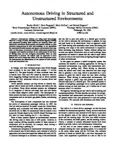
D. Movement Planning Another Application is movement planning on small scales like finding a way around obstacles using short range sensors like camera, lidar, sonar and radar and navigation on the bigger scale with long range sensors like GPS where finding the fastest or most efficient route is important. Huang et al. [25] developed a framework visual path prediction. It consists of two CNNs that separately model the spatial and temporal context as shown in figure 6.
Left camera
Center camera
Right camera
Steering wheel angle (via CAN bus)
Fig. 5: Maneuver anticipation pipeline. Temporal context in maneuver anticipation comes from cameras facing the driver and the road, the GPS, and the vehicle’s dynamics. (a, b and c) We improve upon the vision pipeline from Jain et al. [19] by tracking 68 landmark points on the driver’s face and including the 3D head-pose features. (d) Using the Fusion-RNN we combine the sensory streams of features from inside the vehicle (driver facing camera), with the features from outside the vehicle (road camera, GPS, vehicle dynamics). (e) The model outputs the predicted probabilities of future maneuvers.
5
Figure 7. Jain’s et al. [27] system architecture for driver activity anticipation: First the face is tracked (a) in the next step the feature vectors for inside and B. 3D head pose and facial landmark features outside context are computed (b), which are fed into the RNN (c+d)anticipation to We then now propose new features for maneuver finally get the manoeuvre prediction (e). which significantly improve upon the features from Jain et
al. [19]. Instead of tracking discriminative points on the driver’s face we use the Constrained Local Neural Field (CLNF) model TM [3] and track 68 fixed landmark points on NVIDIA DRIVE PX is particularly well suited for driving the driver’s face. CLNF scenarios due its ability to handle a wide range of head pose and illumination variations. As shown in Figure 6 CLNF Figure 1: High-level view of the data collection system. offers us two distinct benefits over the features from Jain et al. [19] (i) while discriminative facial points may change from situation to situation, tracking fixed landmarks results in consistent optical flow trajectories which adds to robustness; Fig. 6: Improved features for maneuver anticipation. We track Images for two specific off-center shifts can be obtained fromalso theallows left us and the right Adand (ii) CLNF to estimate the camera. 3D head pose facial landmark points using the CLNF tracker [3] which results in of the face by by minimizing error in the projection of aof ditional shifts2Dbetween the cameras all rotations aredriver’s simulated viewpoint transformation more consistent trajectories as compared to the and KLT tracker [32] used by Jain et al. [19]. Furthermore, the CLNF also gives an generic 3D mesh model of the face w.r.t. the 2D location of the image from the nearest camera. Precise viewpoint transformation requires 3D scene knowledge estimate of the driver’s 3D head pose. landmarks in the image. The histogram features generated which we don’t have. We therefore approximate the transformation by assuming all points below from the optical flow trajectories along with the 3D head anticipation. Figure 5 shows our complete pipeline. In order the horizon maneuvers, are on flatourground and all points thefeatures horizon arepitch infinitely (yaw, and row),far giveaway. us xt 2This R12 . works to anticipate RNN architecture (Figureabove 4) pose fine for flat it introduces for objects thatVIstick aboveresults the ground, asfrom cars, processes the terrain temporalbut context {(x1 , ..., xt ),distortions (z1 , ..., zt )} at In Section we present with the such features Fig. 3. The overview of our framework. Spatial Matching Network and Orientation Network are two CNNs, which respectively model the spatial and every time step t, and outputs softmax probabilities y for Jain et al. [19], as well as the results with our improved trees, and buildings. Fortunately theset distortions don’t pose a big problem for network traintemporal contexts. We repeatedly input images of the object and local environment patches into Spatial Matching Network to generate the reward map of the Figure 6.it helps Overview Huang’s et al. framework. the object of poles, scene. Intuitively, us decide whetherof the object could reach certain areas [25] of the scene. Orientation Network First estimates the object’s facing orientation, the following five maneuvers: M = {left turn, right turn, left features obtained from the CLNF model. ing. The steering label for transformed images is adjusted to one that would steer the vehicle back which indicates the object’s preferred moving direction in the future. Then we incorporate this analysis and infer the most likely future paths with a unified interest is cropped out with a bounding box (red). The rest of the image is tolane change, right lane change, straight driving}. We now path planning scheme. thean desired location and orientation in two seconds. VI. E XPERIMENTS overview of the feature representation used by Jain then divided into local environment patches of the same size as the object give We evaluate our proposed architecture on the task of et al. [19] and then describe our features which significantly A block diagram of our training system is shown maneuver in Figureanticipation 2. Images are27, fed36]. into a CNN which [1, 19, This is an impor(dotted Thea scene spatial network gets fed with the object plus improve the performance. for an objectblue). Iobject and image matching I by repeatedly then computes a proposed steering command. Thetant proposed command is US compared to the desired Facing orientation θ problem because in the alone 33,000 people die inputing all the local environment patches q with the same an environment patch (yellow) at each time to generate a reward map of in road accidents every yearthe – aCNN majority of which areto object patch Iobject into Spatial Matching Network: fc9 (1) command image and the weights of the CNN are adjusted to bring output closer A. Featuresfor for that maneuver anticipation fc8the (64) the scene. The orientation networks estimatesfc7fc7(4096) object’s facing orientation due to dangerous maneuvers. Advanced as Driver Assistance frame t (4096) the desired output. The weight adjustment is accomplished using back propagation implemented Rreward (si ) = FS (Iobject , qsi ; S ). (6) In the vision pipeline of Jain et al. [19], the driver Systems (ADAS) have made driving safer by alerting drivers fc6 (4096) frame t+1 to indicate the object’s preferred movementpool5direction for future steps. They infacing the Torch machine learningpoints package. (3×3, 256, 2) camera 7detects discriminative on the driver’s whenever they commit a dangerous maneuver. Unfortunately, Rreward (si ) 2 [0, 1] is the reward r for each position si . The conv5 (3×3, 256, 1) face and tracks the detected points across frames using the many accidents are unavoidable because by the time drivers bothvalue serve inputreward forforthe unified path planning conv4 (3×3, 384, 1) scheme. Finally, the path larger meansas the higher that position, namely conv3 (3×3, 384, 1) KLT tracker [32]. The tracking generates 2D optical flow are alerted it is already too late. Maneuver anticipation can the higher probability object will reachon thatthe position in the image LRN2 predictions arethedisplayed input trajectories in the image plane. From these trajectories the avert many accidents by alerting drivers before they perform pool2 (3×3, 256, 2) future. Visualization of our reward maps generated on different Recorded conv2 (5×5, 256, 1) horizontal and angular movements of the face are extracted, a dangerous maneuver [30]. LRN1 scenes are shown in the middle column of Fig. 7. steering pool1 (3×3, 96, 2) and these movements are binned into histogram features for It is noted that the reward function in the previous work conv1 (11×11, 96, 4) We evaluate on Desired the drivingsteering data set command publicly released by wheel angle Adjust for every frame. These histogram features are aggregated shift over 20 [4, 5] only models the scene itself. However, different objects Object patch I frames (i.e. 0.8 seconds of driving) and constitute the feature Jain et al. [19]. The data set consists of 1180 miles of and rotation may have different relationships with the same region of the natural freeway and city driving collected from 10 drivers 9 vector xt 2 R . Further context for anticipation comes scene. So the reward map in our method is built with respect over a period of two months. It contains videos with both to both of the specific object and the scene appearance, for the Fig. 5. Illustration of Orientation Network. What is the facing orientation from the camera facing the road, the GPS, and the vehicle’s inside and outside views of the vehicle, the vehicle’s speed, 6 purpose of generalization across a diverse set of scenes and of the given object? We train Orientation Network to estimate it accurately. dynamics. This is denoted by the feature vector zt 2 R , Network set is annotated with 700 The network takes an object image Iobject as input. It outputs the estimated and includes objects. the lane information, the road artifacts such as and GPS coordinates. The data Left camera computed facing orientation angle ✓esti of the object. The architecture from conv1 events consisting of 274 lane changes, 131 turns, and 295 The reward map Rreward can be converted to the cost map to fc7 is similar to AlexNet [36]. We add fc8 and fc9 to reduce features’ intersections, and the vehicle’s speed. We refer the reader to randomly sampled instances steering of driving straight. Each lane Rcost , such that: dimension, followed by a regression layer. The relative position of the same Jain et al. [19] for more information on their features.
External solid-state drive for data storage
F. End-to-End
The previously mentioned End-to-End approach has recently received a lot of attention as Bojarski et al. of Nvidia [28], [29] introduced their later called PilotNet system. PilotNet is a CNN consisting of nine layers in total including a normalization layer, five convolutional layers and three fully connected layers. The whole system architecture for training is shown in figure 8. Finally the trained system is able to drive on the road with just one centred camera as input signal.
esti
For training 8.5 hours of the VIRAT Video Dataset containing 11 different outdoor scenes and for testing the smaller KIT AIS dataset consisting of 9 different outdoor scenes was used. The results were compared to state-of-the-art nearest neighbour command Random shift and mid-level element algorithmic approaches, which both 1 Center camera CNN R (s) = , (7) and rotation 3122 1+e were outperformed on all scenes by accuracies around 30%. where ↵ is the tolerance to obstacles. is fixed to 0.5, as the appearance and the spatial position. As the information about Right camera scale of R (s) is [0, 1].let’s Based ontheir this formulation, we can Drive.ai [26] small fleet ofappearance four has autonomous Audis physical been integrated in Spatial Matching compute the spatial matching cost C of a path P according Network, we only model the position variation of object itself, Error to Eq. (2). Back propagation even take one further step. Theirnamely carsthedo decision andtime. relative position of themaking object at different weight adjustment When in the test phase, it is represented as the object’s facing motion planing on difficult situations like theofAmerican C. Orientation Network orientation with the input a single image. Thefour temporal In this subsection, we discuss how to build Orientation Net- context also plays an important role in selecting the future way stop, where thevideofirst come first serveimagine rulea man is walking applied, or he For instance, on the street; work to learn the temporal context from sequences in the path. Figure 2: Training the neural network. training phase, and, to estimate an object’s facing orientation is most likely to walk along his facing orientation. Similarly, Figure 8. Nvidia’s [28] end-to-end training set-up: Training data is collected red, which inobject most any kind of active follows intersections. this rule if there are no other ✓even in theturning testing phase. on Because the scene is assumedisto allowed via the video signals of three behind the wind shield mounted cameras be static in the visual path prediction task, we only focus on external factors disturbing it. The the small claims be we able to build 4 anOnce trained, the network can generate steering the video images a single center modeling temporal tech-startup context of the object itself. In other to Therefore, build Orientation Networklevel to estimate combined with the steering wheel anglefrom received by the car’sofCAN-Bus. Thecamera. words, we are going to model the time-dependent variation object’s facing orientation ✓ . The architecture of OrienThis configuration is shown in Figure 3. autonomous systems in the nexttationyears, means selfof the object’s own state. The state here includes the physical Network iswhich shown in Fig. 5. We firstaextract image CNN computation happens in a Nvidia Drive Px, which is the predecessor driving system that doesn’t require human intervention in most model of the already mentioned GPU system. The output is a steering command 1/r, where r is the turning 3radius in meters, which is constantly scenarios. compared to the real steering angle to adjust the weights via backpropagation. object
object between neighbouring frames serves as the ground truth label.
cost
↵(Rreward (s)
)
-
reward
S
esti
esti
E. Driver State The Driver State surveillance task is to predict the driver’s future actions. Jain’s et al. [27] developed a system called Driver activity anticipation (DAA) which uses a similar network architecture as SVTA. The system fuses the sensor inputs of a cockpit camera that tracks the driver’s face movement and the sensors that understand the outside context like GPS and outside cameras. In order to anticipate upcoming manoeuvres the Network learns to predict the future driver manoeuvres given only a partial temporal context. This is possible through the special RNN structure with LSTM units, that are trained to map all sequences of partial observations to the future event as shown in figure 7. With this system a precision of 90.5% and a recall of 87.4% is achievable on a training set of 1180 miles natural driving.
An important part of their training process was the already mentioned data augmentation technique because training with data only from an human driver is not sufficient. They randomly altered images in the training process where the car was shifted or rotated on the road.
The most interesting part is that the car needs no other DL system or classical control unit for autonomy, everything happens inside PilotNet. It learns how to steer the vehicle by being trained on the data collected from a human pilot drive along different roads for 72 hours. If looked at the activation maps of different layers inside PilotNet as shown in figure 9 it becomes clear that it learned to detect useful road features like road lines without ever been taught what a road looks like. Besides highway driving it also manages to steer safely on offroad ways or through cones on parking lots, as it recognizes the outlines of what are meant to be roads in completely different scenarios.
ADVANCED SEMINAR SS 2017: SURVEY OF NEURAL NETWORKS IN AUTONOMOUS DRIVING
Figure 7: How the CNN “sees” an unpaved road. Top: subset of the camera image sent to the CNN.
Figure 9.left:PilotNet’s and second layer outputs forof the ansecond inputlayer image Bottom Activation of [28] the firstfirst layer feature maps. Bottom right: Activation maps. Thispathway. demonstratesThe that the CNN learnedmaps to detectrecognize useful road features on its own, i. e., of feature an off-road activation the road’s features, with only the human steering angle as training signal. We never explicitly trained it to detect the visible byof the outlines roads.white lines standing out of the black background.
This section took a glance at recent research projects of neural networks and deep learning in the field of autonomous driving. Before the discussion to what extend the four given questions can already be answered, the next section takes a closer look at the strengths and weaknesses of deep learning to be finally able to give a outlook about future possibilities. III. A DVANTAGES AND HINDRANCES IN THE USE OF D EEP L EARNING Deep Learning has several convincing advantages over classical algorithmic or robotical control approaches. Nevertheless, Figure 8: Example image with no road. The activations of the first two feature maps appear to it contain also mostly hasnoise, toi. e.,overcome a useful fewfeatures significant the CNN doesn’t quite recognize any in this image. technical hurdles. In this section the advantages and hindrances of DL 8 are examined.
A. The Bright Side 1) Improvement through Learning: One major argument why deep learning is the driving force to achieve autonomous driving is because it makes machines steadily improve through learning. Andrew Ng, chief scientist of Baidu [30] claims DNNs keep improving with the amount of data available for learning where other machine learning algorithms already reach their limit as shown in figure 10. Moreover, Reinforcement learning enables learning from experience instead of having programmed every step and turn by man. In contrast to other methodologies, deep learning does not need hand crafted features. It learns simple features in the lower shallow layers as well as complex ones with increasing layer depth on its own. Learning in this case means that the DNN is fed huge amounts of input data to gradually improve the output prediction by minimizing the cost function through iterativley adjustment of the Nets’ weights in the hidden layers. DL reacts better in unseen scenarios than rule-based approaches as it can adapt into complex situations where classical rule based control fails [31]. If a difficult situation is encountered, the data is collected and the deep learning brain is trained on it so it knows how to react or decide the next time a similar situation occurs [26].
5
Figure 10. Andrew Ng’s [30] graph shows how deep learning is said to outperforms traditional learning algorithms with increasing amount of available training data.
2) Computation Power: Although NNs have been known for decades, their development stuck until ten years ago as hardware was not advanced enough to collect, store and process the massive amount of data necessary to properly train DNNs. This changed with the availability of powerful Graphic Processing Units (GPU), which perform many calculations at once aswell as data storages in huge sizes at very low cost. They are able to shorten the time necessary for training a big network from days or weeks down to hours, hence the computing task is no barrier any more claims Shapiro, Senior Director of Automotive at Nvidia [32], [33]. Nvidia is one of the leading developers for GPUs that are mastering the complex computation tasks while training and enabling real-time decision making while driving. They developed an all-in-one system especially for online computation in autonomous cars named Nvidia Drive Px 2 [34]. With each two mobile procesessors and GPUs It can operate up to 24 trillion mathematical operations per secound and can be stacked parallel for further performance increase. As confirmed by Nvidea [35] Tesla is using the Drive Px 2 System for its autopilot systems in all three models since late 2016 as it has 40 times more computing power than their old system. 3) Knowledge and Software Availability: Setting up a theoretical complex DNN, like a CNN described in the introduction, is easy to handle with now available resources. With open source programming libraries such as Tensorflow of Google or Caffe of Berkley University it is possible to build up and train DNNs as well as to validate the results afterwards with minimum programming knowledge. The open source documentation about DL via blogs, tutorials or youtube videos is massively increasing since 2015 as it is a field of research that attracts a lot of young data scientists. Compared to classical rule based decision making just a few lines of code and thereby expert knowledge is necessary to get started working on the topic. 4) Performance: Finally, the most important reason why DL is the future of autonomous driving is performance. DNNs had their breakthrough around 2012 with AlexNet winning the ImageNet competition, which is basically the ”annual olympics of computer vision”, by dropping the actual best error rate record
6
ADVANCED SEMINAR SS 2017: SURVEY OF NEURAL NETWORKS IN AUTONOMOUS DRIVING
from 26% to 16% [14]. This led to dropping classification errors every year through various systems as shown in figure 11. Since then DNNs, in particular CNNs outperform any other form of machine learning approach by orders of magnitude especially at Computer Vision applications such as object detection and classification. ImageNet ClassificaHon Error (Top 5) 30,0
25,0
26,0
20,0
16,4
15,0
11,7
10,0
7,3
5,0
6,7
5,0
3,6
3,1
2015 (ResNet)
2016 (GoogLeNet-v4)
0,0
XRCE 2011 (XRCE)
2012 (AlexNet)
2013 (ZF)
2014 (VGG)
2014 (GoogLeNet)
Human
Figure 11. Winner results of the ImageNet large scale visual recognition challenge (LSVRC) of the past years on the top-5 classification task: The green bar indicates the best computer vision approach, whereas the blue bars are all deep neural network architectures. The human score is represented as the red bar. (The values for the diagram are compiled from the image-net homepage [36]).
B. The Dark Side 1) Labelled Data: Most DNNs are trained with supervised learning that requires massive amounts of labelled training and testing data. Having enough labeled data is important, as DNNS tend to overfit. An indication for overfitting, due to too little training data, is when the error on the training dataset is already small but the error on an unseen test set is still high. To overcome this problem companies employ thousands of people to label their data. It is approximately 800 hours of work labelling collected driving footage to recieve one hour of usable data [26] as every video frame is basically one image, which makes 108, 000 images to be labelled at 30 frames per secound (fps). Therefore Amazon hosted a platform called Mechanical Turk [37]. It is a service to outsource the labelling of data to companies and schools in low wage countries. Although it provides reasonable results, supporting it is questionable. 2) Sensor Fusion: Another big challenge is sensor fusion as it is especially difficult to filter unneeded information and to fuse the different kind of data provided by sensors working on an autonomous car. Possible sensor signals include cameras, lidar, radar, GPS, ultrasonic, Infra-red and audio, moreover driver signals such as steering angle, brakeand acceleration pedal position and finally vehicle dynamic signals such as speed, yaw rate, damper force and wheel slip. To refine this wast amount of information collected by sensors to make them suitable for training is one major hindrance to autonomous driving because it still needs lots of man working power.
3) Blackbox Problem: DNNs are often seen as Blackboxes [26], this is especially problematic in end-to-end realizations. The fact that it is not really visible what happens inside the hidden layers between in- and output and how it finally gets to its solution is the reason a lot of companies hesistate to use DNNs. Furthermore, troubleshooting and debugging can sometimes be a hard task the deeper a network gets. Especially in applications concerning the security of human life it is absolutely necessary to know exactly what the system does. It is one major hindrance to first collect enough training data of so called ”corner cases”, situations in autonomous driving that are extremely rare but dangerous at the same time, and later validate the behaviour of the network in those cases [19]. 4) Manipulability: Although DNNs perform robust in various conditions, they are not completely secure against manipulation. In 2013, a Group of Scientists from Google, Facebook and some major US Universities published a paper where they were able to spoof at that time state-of-the-art DNNs such as AlexNet with putting filters or minimal distortions over test pictures that a human eye can’t even recognize but led the DNNs to drop their accuracy by a factor of ten. This Problem is not limited to camera signals, also other sensors like Lidar are spoofable with similar tricks [38]. To overcome this problem, techniques like the previously mentioned data augmentation or batch normalization, introduced by Ioffe et al. [39] to reduce covariate shift, are used. 5) Safety Validation: The final challenge is to make security and safety validation of DNNs in autonomous driving meet auto industy standards as they calculate stochastic results that are likely to make false positive and false negative decisions [19]. The human level safety is said to be near a mean time between failure of 109 hours. It would take a fleet of million cars that operates one hour a day thousand days of testing to see one catastrophic failure. In fact, you must repeat testing several times to achieve statistically signifcant statements. Furthermore, it is impossible to test every corner situation that may occur due to exponentially exploding combination possibilities of different kind of impacts such as sensor or system failure, weather conditions, unusual behaviour of other road users and many more. To cope with these blind spots in the safety validation of DNNs a relatively mature testing technology could be fault injection. The reason why very high Automotive Safety Integrity Levels (ASIL) [40] must be achieved with full autonomy is that there might be critical situations where the driver does not have the ability to take corrections, instead the computer system must handle any fault or risk occurance. An approach to lessen this Problem is to use ASIL-decomposition where a monitor/actuator architecture is used. The monitor is designed with high level ASIL while the actuator can work on a lower level. In combination with heterogeneous redundancy the ASIL level is further increased and the system is able to do a saftey fail-stop if necessary. This section examined the advantages and hindrances
REFERENCES
connected to the use of deep learning. It showed that former hindrances like computation power are already solved, whereas recent hurdles like safety validation are already in the progress. In the subsequent sections the main results of this report are summarized and discussed. IV. D ISCUSSION AND F UTURE O UTLOOK This final section contains the discussion about how far research actually is and which approaches seem to be most promising. This is followed by a brief future outlook about interesting methodologies before the eventual conclusion. A. Discussion Summarizing the presented applications it is safe to say that besides object detection as well as classification and localization applications using CNNs, which already perform on series or close to series level, most Deep Learning applications for autonomous driving still need further research. This also applies to applications which already work well on their tested scenarios like Nvidia’s End-to-End approach. But validating those systems for auto industry standards is a completely different story as they face the blackbox problem. A possibility to get these applications closer to series would be if they are not supposed to work on full autonomy but customized to fulfil lower level driver assistance tasks where the driver is still kept in charge. The most promising research fields are thereby recurrent neural networks in combination with long short term memory approaches as they are able to learn long term dependencies to predict future actions, which is substantial to achieve autonomous driving. Eventually, being able to handle networks that use sensor fusion is the key to achieve high safety levels, for example to use radar signal to detect false negatives in object detection by the camera system. Finally, state-of-the-art methods of deep learning are at least partially able to answer the previous raised questions concerning localization, mapping, scene understanding, movement planing and driver state.
7
recognize different driving styles, to be able to adapt the car’s dynamics behaviour if the driver changes between smooth or sporty driving to maximize driving pleasure as well as safety and comfort. V. C ONCLUSION This report gave a brief introduction into the wide area of deep learning. Convolutional and recurrent neural networks have been presented as the benchmark for their respective application fields, object detection and long term planning. Furthermore, current state-of-the-art applications including amongst others, End-to-End approaches, driver state and scene understanding have been illuminated. Moreover, the advantages and hindrances connected to the use of deep learning have been examined. With the result that many hurdles, like safety validation or the necessary amount of training data are already in the progress of being solved. Eventually the decisive argument why deep neural networks will prevail is their high performance enhanced due to the availability of powerful computation components. Ultimately, should not be underestimated that even if research is making great progress, there is still a long way to achieve autonomous driving. R EFERENCES [1] [2] [3] [4]
[5]
[6]
[7]
B. Future Outlook While gathering information for this report the author came across some interesting methodological approaches where unfortunately not enough documentation was available. As most networks are trained on supervised learning a promising strategy could be to use unsupervised learning to pre-label training data to save huge amount of time as only the label validation would remain as a human task. Furthermore, the combination of CNNs and RNNs that use reinforcement learning to create networks that are able to do high performance vision based motion planning tasks. Another application is to survey the driver’s mental condition to timely recognize if he faces health problems or is likely to fall asleep to be able to give warn signals or to take over control. Moreover, simulating training data especially for corner cases is a promising approach as the validation of Deep Learning systems is still a not yet reached goal. Finally, a drive style to active chassis application could be interesting, where a Deep Learning system is trained to
[8] [9] [10] [11] [12] [13] [14] [15]
I. Goodfellow, Y. Bengio, and A. Courville, Deep Learning. MIT Press, 2016. Y. LeCun, Y. Bengio, and G. Hinton, “Deep learning”, Nature, vol. 521, no. 7553, pp. 436–444, 2015. L. Fridman, “Learning to drive: Convolutional neural networks and end-to-end learning of the full driving tasks”, MIT, Course 6.S094, Tech. Rep., 2017, lecture 3. L. Jing, T. Wang, M. Zhao, and P. Wang, “An adaptive multi-sensor data fusion method based on deep convolutional neural networks for fault diagnosis of planetary gearbox”, Sensors, vol. 17, no. 2, p. 414, 2017. B. Wu, F. Iandola, P. H. Jin, and K. Keutzer, “Squeezedet: Unified, small, low power fully convolutional neural networks for real-time object detection for autonomous driving”, ArXiv preprint arXiv:1612.01051, 2016. J. Morton, T. A. Wheeler, and M. J. Kochenderfer, “Analysis of recurrent neural networks for probabilistic modeling of driver behavior”, IEEE Transactions on Intelligent Transportation Systems, vol. 18, no. 5, pp. 1289–1298, 2017. V. Nair and G. E. Hinton, “Rectified linear units improve restricted boltzmann machines”, in Proceedings of the 27th international conference on machine learning (ICML-10), 2010, pp. 807–814. M. D. Zeiler and R. Fergus, “Stochastic pooling for regularization of deep convolutional neural networks”, ArXiv preprint arXiv:1301.3557, 2013. (26-06-2017). Understanding lstm networks, [Online]. Available: http: //colah.github.io/posts/2015-08-Understanding-LSTMs/. L. Fridman, “Learning to move: Deep reinforcement learning for motion planning”, MIT, Course 6.S094, Tech. Rep., 2017, lecture 2. J. Ngiam, A. Khosla, M. Kim, J. Nam, H. Lee, and A. Y. Ng, “Multimodal deep learning”, in Proceedings of the 28th international conference on machine learning (ICML-11), 2011, pp. 689–696. J. Yosinski, J. Clune, Y. Bengio, and H. Lipson, “How transferable are features in deep neural networks?”, in Advances in neural information processing systems, 2014, pp. 3320–3328. D. Cires¸An, U. Meier, J. Masci, and J. Schmidhuber, “Multi-column deep neural network for traffic sign classification”, Neural Networks, vol. 32, pp. 333–338, 2012. A. Krizhevsky, I. Sutskever, and G. E. Hinton, “Imagenet classification with deep convolutional neural networks”, in Advances in neural information processing systems, 2012, pp. 1097–1105. X. Chen, K. Kundu, Z. Zhang, H. Ma, S. Fidler, and R. Urtasun, “Monocular 3d object detection for autonomous driving”, in Proceedings of the IEEE Conference on Computer Vision and Pattern Recognition, 2016, pp. 2147–2156.
8
[16]
[17] [18] [19] [20]
[21] [22]
[23]
[24] [25]
[26] [27]
ADVANCED SEMINAR SS 2017: SURVEY OF NEURAL NETWORKS IN AUTONOMOUS DRIVING
B. Dong and X. Wang, “Comparison deep learning method to traditional methods using for network intrusion detection”, in Communication Software and Networks (ICCSN), 2016 8th IEEE International Conference on, IEEE, 2016, pp. 581–585. J. Long, E. Shelhamer, and T. Darrell, “Fully convolutional networks for semantic segmentation”, in Proceedings of the IEEE Conference on Computer Vision and Pattern Recognition, 2015, pp. 3431–3440. V. Badrinarayanan, A. Kendall, and R. Cipolla, “Segnet: A deep convolutional encoder-decoder architecture for image segmentation”, ArXiv preprint arXiv:1511.00561, 2015. T. Dubner, P. Edin, B. Lakshman, and Y. Suganuma, “I see. i think. i drive. (i learn)”, KPMG, 2016. B. Huval, T. Wang, S. Tandon, J. Kiske, W. Song, J. Pazhayampallil, M. Andriluka, P. Rajpurkar, T. Migimatsu, R. Cheng-Yue, et al., “An empirical evaluation of deep learning on highway driving”, ArXiv preprint arXiv:1504.01716, 2015. J. Redmon and A. Farhadi, “Yolo9000: Better, faster, stronger”, ArXiv preprint arXiv:1612.08242, 2016. A. Khosroshahi, E. Ohn-Bar, and M. M. Trivedi, “Surround vehicles trajectory analysis with recurrent neural networks”, in Intelligent Transportation Systems (ITSC), 2016 IEEE 19th International Conference on, IEEE, 2016, pp. 2267–2272. C. Chen, A. Seff, A. Kornhauser, and J. Xiao, “Deepdriving: Learning affordance for direct perception in autonomous driving”, in Proceedings of the IEEE International Conference on Computer Vision, 2015, pp. 2722–2730. (26-06-2017). Welcome to the kitti vision benchmark suite!, [Online]. Available: http://www.cvlibs.net/datasets/kitti/. S. Huang, X. Li, Z. Zhang, Z. He, F. Wu, W. Liu, J. Tang, and Y. Zhuang, “Deep learning driven visual path prediction from a single image”, IEEE Transactions on Image Processing, vol. 25, no. 12, pp. 5892–5904, 2016. E. Ackermann, “How drive.ai is mastering autonomous driving with deep learning”, IEEE Spectrum, 2017. A. Jain, A. Singh, H. S. Koppula, S. Soh, and A. Saxena, “Recurrent neural networks for driver activity anticipation via sensory-fusion architecture”, in Robotics and Automation (ICRA), 2016 IEEE International Conference on, IEEE, 2016, pp. 3118–3125.
[28]
[29]
[30] [31]
[32]
[33] [34] [35] [36] [37] [38] [39] [40] Safety,
M. Bojarski, D. Del Testa, D. Dworakowski, B. Firner, B. Flepp, P. Goyal, L. D. Jackel, M. Monfort, U. Muller, J. Zhang, et al., “End to end learning for self-driving cars”, ArXiv preprint arXiv:1604.07316, 2016. M. Bojarski, P. Yeres, A. Choromanska, K. Choromanski, B. Firner, L. Jackel, and U. Muller, “Explaining how a deep neural network trained with end-to-end learning steers a car”, ArXiv preprint arXiv:1704.07911, 2017. (25-06-2017). Andrew ng, chief scientist of baidu, [Online]. Available: http://www.andrewng.org. M. Copeland. (24-06-2017). What’s the difference between artificial intelligence, machine learning, and deep learning?, [Online]. Available: https://blogs.nvidia.com/blog/2016/07/29/whats- differenceartificial-intelligence-machine-learning-deep-learning-ai/. B. Lewis. (24-06-2017). Educating the auto with deep learning for active safety systems, [Online]. Available: http : / / embedded computing . com / articles / educating - the - auto - with - deep - learning for-active-safety-systems/. D. Shapiro. (24-06-2017). Here’s how deep learning will accelerate self-driving cars, [Online]. Available: https://blogs.nvidia.com/blog/ 2015/02/24/deep-learning-drive/. (25-06-2017). Neueste version der nvidia drive px 2, [Online]. Available: http://www.nvidia.de/object/drive-px-de.html. (25-06-2017). Tesla and nvidia, [Online]. Available: http : / / www . nvidia.com/object/tesla-and-nvidia.html. (28-06-2017). Imagenet lsvrc challenge, [Online]. Available: http:// image-net.org/challenges/LSVRC. (24-06-2017). Amazon mechanical turk, [Online]. Available: https : //www.mturk.com/mturk/welcome. C. Szegedy, W. Zaremba, I. Sutskever, J. Bruna, D. Erhan, I. Goodfellow, and R. Fergus, “Intriguing properties of neural networks”, ArXiv preprint arXiv:1312.6199, 2013. S. Ioffe and C. Szegedy, “Batch normalization: Accelerating deep network training by reducing internal covariate shift”, in International Conference on Machine Learning, 2015, pp. 448–456. P. Koopman and M. Wagner, “Challenges in autonomous vehicle testing and validation”, SAE International Journal of Transportation vol. 4, no. 2016-01-0128, pp. 15–24, 2016.