Saeid Veysi Raygani, Bijan Moaveni, Seyed Saeed Fazel, Amir Tahavorgar
WSEAS TRANSACTIONS on CIRCUITS and SYSTEMS
SVC Implementation Using Neural Networks for an AC Electrical Railway SAEID VEYSI RAYGANI, BIJAN MOAVENI, SEYED SAEED FAZEL, AMIR TAHAVORGAR Electrical Railway Engineering Iran University of Science and Technology Hengam Street, Narmak, Tehran IRAN
[email protected],
[email protected],
[email protected],
[email protected] Abstract: - This paper presents an on-line method for implementation of a static var compensator (SVC) in a real ac autotransformer (AT)-fed electrical railway for reactive power compensation using Neural Networks (NN). Genetic algorithm (GA) can be the off-line minimizing function for reactive power compensation. Consequently, the nonlinear auto-regressive model with exogenous Inputs networks in series-parallel arrangement (NARXSP) is implemented as a predictor and methodology in order to diminish calculation time and making this method practicable. To study load flow and reactive power compensation for this unique system, forward/backward sweep (FBS) load flow method is applied. MATLAB software is used for programming and simulations. Key-Words: - Neural network (NN), reactive power compensation, static var compensator (SVC),
genetic algorithm (GA), AC electrical railways load flow, forward/backward sweep (FBS). unbalanced single phase ac AT-fed railway networks and applied for Tehran-Golshahr suburban electrical railway for study optimal power flows. In this paper, Reactive power compensation by use of a single-phase static var compensator (SVC) installed at the sectioning point (SP) is studied. In order to minimize the power losses by the single phase SVC, swift and accurate methods are needed to analyze the network and calculate amounts of needed reactive power. Kulworawanichpong and Goodman, in [10] for a simple mode (SM) railway system, stated that gradient search method (steepest descent method) is sufficient for minimizing power losses. Their objective function was proportional to the square of voltage or reactive power variations and they claimed that their methodology solves minimizing function precisely and in an appropriate time. In this paper, however, the compensation function minimizes the imaginary part of the current in a whole real electrical system. Genetic algorithm (GA) is considered as a comprehensive and global minimizing function method. GA is time consuming and consequently cannot be a good solution for realtime implementation. Thus, neural networks, which can approximate the complicated functions thorough a training procedure, are taken into account to save the time and make implementation of the SVC feasible. The nonlinear auto-regressive model with
1 Introduction Recently, electrical ac railways using 25kV, 50Hz are playing leading roles in urban transportation systems [1]. Asynchronous train tractions lead to drastic changes in both currents and power profiles of the traction substation (TSS). It is desirable to mitigate these effects as low as possible by reactive compensation methods applied in optimal power flow. On the other hand, However, Solving load flow problems and consequently optimal power flows in these systems are always a complex problem because of trains types, trains motion, variable power consumption, route lengths and conditions, dispatch schedules, and track and supply system layouts [2]-[6]. In autotransformer (AT)-fed networks, this issue gets more complicated due to the AT characteristics in load feeding and necessity of voltage drop calculations on the contact and feeder wires as well as the rail [4]-[6]. One of the main studies for the AT-fed load flow was conducted in 1999 [4] which considered only one train between two ATs while dynamic movements of trains were not considered. Reference [5] presents probabilistic load flow models which simplify railway load flow analysis. The forward/backward sweep (FBS) load flow method is widely used for load flow calculation in distribution systems [7]-[9]. In this paper, this method is modified for
ISSN: 1109-2734
173
Issue 5, Volume 10, May 2011
Saeid Veysi Raygani, Bijan Moaveni, Seyed Saeed Fazel, Amir Tahavorgar
WSEAS TRANSACTIONS on CIRCUITS and SYSTEMS
(C), rail (R), and feeder (F), respectively. So, (2) is obtained regarding the variation of x.
exogenous Inputs network (NARX) [11] is well suited for non-linear systems such as heat exchangers and waste water treatments plants [12], [13]. In this paper, NARX network in series-parallel arrangement (NARXSP) is considered for calculation of the exact amount of reactive power which must be injected by the SVC. The remainder of the paper is organized as follows. The FBS method which is modified for ac electrical AT-fed railways is presented in section 2. Minimizing reactive power and the methodology using neural network is discussed in sections 3. Simulation results are given in section 4. Section 5 presents the conclusions of this work.
⎡U C ⎤ ⎡ I C ⎤ ⎡U C ( x ) ⎤ ⎢U ⎥ = Z (x ) ⎢ I ⎥ + ⎢U x ⎥ ] ⎢ R ⎥ ⎢ R ( )⎥ ⎢ R⎥ [ ⎢⎣U F ⎥⎦ ⎢⎣ I F ⎥⎦ ⎢⎣U F ( x ) ⎥⎦
where IC represents catenary current, which can be changed by charging currents of coupling capacitors between the catenary and both the rail and feeder. However, coupling capacitors and consequently charging currents are small enough to be neglected [14]. PQ busses (trains) move along the track and consequently x changes. Therefore, load flow calculations must be iterated for each location, x.
2 Load Flow Calculations For unbalanced distribution systems, the impedance matrix consists of the self and mutual equivalent impedances for the three phases. The model depicted in Fig.1 constitutes the fundamental part of the computational method that simultaneously analyzes the three lines and their reciprocal interactions. Thus, (1) allows expressing the sending voltages, Uai, Ubi, and Uci, with branch currents, Ia, Ib, and Ic; and receiving voltages, Uaj, Ubj, and Ucj.
⎡U ai ⎤ ⎡ I a ⎤ ⎡U aj ⎤ ⎢U ⎥ = Z (x ) ⎢ I ⎥ + ⎢U ⎥ ] ⎢ b ⎥ ⎢ bj ⎥ ⎢ bi ⎥ [ ⎢⎣U ci ⎥⎦ ⎢⎣ I c ⎥⎦ ⎢⎣U cj ⎥⎦
2.1 AT systems ATs lead to changes in the feeding currents and flowing currents from the TSS. In the load flow calculation, following key points are taken into account: a) the TSS transformer is modeled as a single phase transformer and an AT, whose midpoint connected to the rails with zero potential; b) ATs are regarded as ideal voltage sources whose voltages will be calculated after load flow calculations. As shown in Fig.2, ATs secondary currents, I2n, feed the train according to (3).
(1)
I 2n =
where x, in Fig.1, represents the distance between sending and receiving points.
Yn
∑
N Y i =1 i
(3)
Il
where
Il =
Pl − jQl V∗
(4)
and Il, V, Pl, and Ql are the current, voltage, active power, and reactive power of the load, respectively. N is the total number of ATs, I2n (n=1, 2, …, N) is the share of secondary current of the nth AT to supply the train, and Yi is the inverse of the aggregate series impedance between the load and ith AT. Isub is the substation current and can be obtained from (5) in which I1i is the primary current and equals 0.5I2i for the ith AT.
Fig.1 Three-phase layout between sending (i) and receiving (j) buses. The FBS method is applied to solve this problem in unbalanced distribution system. In this method, a backward sweep estimates branch powers (or currents). Subsequently, a forward voltage calculation method updates the procedure by applying (1). In (1) and for electric railway systems, the parameters a, b, and c can be replaced with catenary
ISSN: 1109-2734
(2)
N
I sub = ∑ I 1i
(5)
i =1
The procedure for load flow calculations when one train is in the track can be described as follows:
174
Issue 5, Volume 10, May 2011
Saeid Veysi Raygani, Bijan Moaveni, Seyed Saeed Fazel, Amir Tahavorgar
WSEAS TRANSACTIONS on CIRCUITS and SYSTEMS
Fig.2 Current sharing of ATs to suppply one train.
Fig.3 Diagram of an AT electrical raiilway system. a) At first, the voltages of all nodes are considered as 1 per unit. The train current and subsequently all branches currents are calculated based on the train power consumpption (constant power). For current calculations, (3), (4), and (5) are used to obtain each AT current. Eachh AT current is equal to its primary current. In a backkward trend, the current of the rails connected to the last l AT is equal to the summation of the upper and loower of the last AT currents, which are equal to the t feeder and catenary currents of the end section, respectively, as illustrated in Fig.3. Currents for othher sections can be calculated by using KCL law at their corresponding nodes. b) Based on the calculated braanches currents from the previous step, the nodes voltages v can be calculated using (2). So, the train buus voltages can be calculated as follows:
⎡ I C 1,4 ⎤ ⎡U 4 ( x ) ⎤ ⎡U 1 ⎤ ⎢ ⎥ ⎢ ⎥ ⎢ ⎥ ⎢U 5 ( x ) ⎥ = ⎢U 2 ⎥ − [ Z (x ) ] ⎢ I R 2,5 ⎥ ⎢ I F 3,6 ⎥ ⎢⎣U 6 ( x ) ⎥⎦ ⎢⎣U 3 ⎥⎦ ⎣ ⎦
U 1 = −U 3 = 25 kV − Z S 2 × I sub , U 2 = 0 (7) where ZS is the aggregate of o the transmission system transferred impedance to the t railway side (50 kV) and leakage impedance of the t TSS transformer. After calculating voltagges for the PQ bus nodes (4, 5, and 6), other node voltages v can be written as follows: ⎡ I C 4,7 ⎤ ⎡U 7 ⎤ ⎡U 4 ( x ) ⎤ ⎢ ⎥ ⎥ ⎢ ⎥ ⎢ ⎢U 8 ⎥ = ⎢U 5 ( x ) ⎥ − ⎡⎣ Z (d − x ) ⎤⎦ ⎢ I R 5,8 ⎥ ⎢ ⎥ ⎢⎣U 9 ⎥⎦ ⎢U 6 ( x ) ⎥ ⎢⎣ I F 6,9 ⎥⎦ ⎣ ⎦ ⎡ 0.5Z l − A T I C 4,7 ⎤ ⎢ ⎥ − ⎢ 0.25Z l − A T I R 5,8 ⎥ ⎢ ⎥ ⎢⎣ 0.5Z l − A T I F 6,9 ⎥⎦
where Zl-AT is the equivaleent leakage impedance of the AT. It should be mentioned that the magnetic impedance of ATs is negleected. After calculation of all voltages of nodes, for the distance between the second and third AT, U7, U8, and U9 are considered
(6)
where
ISSN: 1109-2734
(8)
175
Issue 5, Volume 10, May 2011
Saeid Veysi Raygani, Bijan Moaveni, Seyed Saeed Fazel, Amir Tahavorgar
WSEAS TRANSACTIONS on CIRCUITS and SYSTEMS
calculation must be in a loop considering each system current effects on the other. Four iterations can minimize the differences. b) The TSS current is equal to half of the summation of the loads currents in the AT system whereas this current for the SM equals to loads summation. In addition, power losses in the AT system are directly related to the number of ATs, length of tracks, and the Overhead Catenary System (OCS) parameters. But, power losses in the SM depends only on the OCS parameters and distance between the load and TSS.
as U1', U2', and U3', respectively. Node voltages for this distance can be calculated in the same way as the previous distance. This forward sweep is followed until the last AT so that the first step of iteration will be completed. Afterwards, the calculated voltages will be used in the next iterative step. Therefore, this procedure is followed like a recursive calculation until the difference between the calculated node voltages for two consecutive steps gets low enough. While more trains are in the track, the solving method is almost the same, but some consideration must be applied: a) for current calculations, superposition is used; so, the currents for ATs are summed up; b) each train adds tree nodes in the distance between two consecutive ATs which must be considered for KVL calculation while using (2); c) while two or more trains are between two consecutive ATs, current of the section which is situated between PQ buses must be calculated by using KCL and this issue must be considered while (2) is used as shown in (9):
⎡U 4 ( x , n ) ⎤ ⎡U 4 ( x ′, n −1) ⎤ ⎢ ⎥ ⎢ ⎥ ⎢U 5 ( x , n ) ⎥ = ⎢U 5 ( x ′, n −1) ⎥ ⎢U 6 ( x , n ) ⎥ ⎢U 6 ( x ′, n −1) ⎥ ⎣ ⎦ ⎣ ⎦ ⎡ I Cn ,n −1 ⎤ ⎢ ⎥ − ⎡⎣ Z (x − x ′) ⎤⎦ ⎢ I Rn ,n −1 ⎥ ⎢ I Fn ,n −1 ⎥ ⎣ ⎦ th
3 Minimizing Reactive Power The power consumption of the electric railway systems depend on the headway, status, and power consumption of trains. Thus, if both on-line data of the trains position and power consumption profiles are available, a central processing system, located at the control room, can specify how much reactive power must be injected to the grid. It is achieved by sending remotely controlled signals from the processing center to compensators to implement reactive power compensation. In this paper, the main objective of the SVC exploitation is minimizing the power losses revealed in (10). To obtain this function, the power losses corresponding to the imaginary component of the current must be compensated to zero as shown in (11).
(9)
th
where n train is farther than the (n-1) train from the TSS and x' is the distance between the (n-1)th train from the predecessor AT (x, and x' < d).
(10)
2 ∀ n , I ny = 0 ⇒ min ( Ploss ) = ∑ n R n I nx
(11)
2
(
2 2 = ∑ n R n I nx + I ny
where Rn and In are the resistance and current of the nth branch of the railway system, respectively. Also, y and x indices indicate the imaginary and real part of the current, respectively.
2.2 Combined System The left side of Tehran-Golshahr network has no installed AT. The distance between TSS and Golshahr station is supplied by SM layout as shown in Fig.4. Power feeding system parameters are given in Appendix. While two systems are connected, load flow calculation should be combined. Following points must be considered to analyze the load flows for this combined system: a) SM has no feeder wire. Thus, load flow calculation in SM is easier and the FBS method as mentioned in subsection A can be implemented. Voltage drop for the loads which are in the AT region must be considered for the loads in SM system and vice versa. For both systems, load flow
ISSN: 1109-2734
)
Ploss = ∑ n R n I n
3.1 Off-line Methodology To reach the global minimum a constrained GA is used. The population consists of initial random set of constrained injected reactive powers due to the SVC. The potential injected reactive powers are the chromosomes forming the population. The arithmetic crossover is shown in (12) in which λ is a random number between 0 and 1, Q represents the chromosome (reactive power), and Q ′ is the offspring [15].
176
Issue 5, Volume 10, May 2011
Saeid Veysi Raygani, Bijan Moaveni, Seyed Saeed Fazel, Amir Tahavorgar
WSEAS TRANSACTIONS on CIRCUITS and SYSTEMS
Fig.4 Tehran-Golshahr power feeding system for up- or down-track.
Q 2′ = Q 2 + (1 − λ )Q1
Q1′ = Q1 + (1 − λ )Q 2
⎛ u (t ), u (t − 1),..., u (t − Du ), yˆ (t − 1), ⎞ ⎟ (15) ⎝ ..., yˆ (t − d y ) ⎠
ˆ =f ⎜ y(t)
(12)
where u(t) and yˆ (t ) describe the input and output of the network at time t. Du and Dy are the input and output orders. The schematic diagram of NARXSP is illustrated in Fig.5.
For mutation (13) is implemented as follows:
X K′ = X K ± Δ (t , X KU − X K )
(13)
where Δ(t , y ) can be defined as below:
t Δ(t, y) = y.r.( 1- ) b T
U(t)
(14)
ˆ Y(t)
Both r and b are the random numbers between 0 and 1, T is the maximal generation number, and t is the generation number.
Y(t)
Fig.5 NARXSP architecture. 3.2On-line Methodology The minimizing function in AT systems is intricate because of sharing currents of AT systems, various power factors of trains, unpredictable current drawn from the TSS, and different headways. The NARXSP network is considered to make power losses minimization feasible by reducing the processing time compared to GA. Based on the definition of the NARXSP, (15) describes the output of the nonlinear function [12], [16], [17]:
The TSS current corresponding to the AT part of the system is considered as an input and the corresponding reactive power of SVC resulted from genetic algorithm is assumed as a desired output. The input vector of the NARXSP model is given by,
⎡ ⎤ ′ I TSS U (t ) = ⎢ ⎥ ⎣⎢cos (angle (I TSS ) ⎦⎥ where
ISSN: 1109-2734
177
Issue 5, Volume 10, May 2011
(16)
Saeid Veysi Raygani, Bijan Moaveni, Seyed Saeed Fazel, Amir Tahavorgar
WSEAS TRANSACTIONS on CIRCUITS and SYSTEMS
′ = I TSS
I TSS
(
max I TSS
improvements of electrical parameters of the system while the SVC compensates the reactive power. Voltage variations for Golshahr (S8) and the SP (S1) are shown in Fig.8. Fig.9 illustrates variations of the TSS currents and voltages. The SVC needs very fast algorithm to implement compensation. Nevertheless, constrained genetic algorithm applied as the power losses minimizing method is not timeefficient. 2) On-line methodology: as described in section 3, we used the NARXSP network to capture and represent the inputs-output relationship. This NN consists of 5 layers and each has 10 neurons. According to definitions in [17], LevenbergMarquardt method is applied as the training method and transfer function of ith layer is tansig, and purelin is considered for the output layer. The performance function and back-propagation network training function are mean squared error (MSE) and trainlm, respectively. Fig.10 shows performance of the trained network during 69 epoches. After learning procedure, the trained neural network calculates precisely the amount of reactive power compared to the results of GA method as shown in Fig.11. In addition, this NARXSP trained neural network gives the corresponding result for various inputs included different magnitude of current and various power factors. Fig.12 shows the results of the NN in comparison with the results of GA for HT=15 while trains work with variable power factors. These results show that the trained neural network, while HT=7 and trains work with PF=0.7, has an ability to compute the required amount of reactive power for the SVC while trains work with various power factor and HT=15 without any delay in reaction to inputs. Thus, the NARXSP network can be considered as an on-line reactive compensator for the SVC regarding the availability of current and its angle measured at the TSS.
(17)
)
In more details, ITSS is the TSS transformer rms ′ , the current corresponding to the AT-side. I TSS magnitude of the normalized traction substation rms current corresponding to the AT-side, is normalized in [0:1] interval. The output vector Y(t) is the normalized reactive power, comprises of QSVC generated by the SVC using GA:
⎡ Q SVC Y (t ) = ⎢ ⎢ max Q SV C ⎣
(
)
⎤ ⎥ ⎥ ⎦
(18)
4 Simulations At first, the detailed model of the railway system is simulated for HT =15 minutes in order to show the results of the written program in MATLAB software. In reactive power compensation section, the reactive powers injected to the system by SVC using GA compose the output vector of the NARXSP model. In this case HT =7 and trains work with PF=0.7. After training, the results of generated reactive power by the SVC using GA while HT=15 and trains work with various power factors above 0.8 is compared with results of the output of the NARXPS network in order to reproduce the identification and validation data sets. The obtained data are processed as described in the next subsections.
4.1 Headway: 15 minutes For HT=15, the time table for the up-track and down-track are given in Fig.6(a) and (b), respectively. Fig.6(c) depicts the speed of the first train which passes the down-track according to the time table. Power consumption for this train is depicted in Fig.6(d). The current simulation for HV side of the TSS is revealed in Fig.7 which implies, in theory, after reaching the stable condition the fluctuations of the current varies periodically in every 15 minutes based on the headway.
5 Conclusion In this paper, the FBS load flow method has been modified for electric AT-fed railways and applied for load flow analysis of Tehran-Golshahr suburban. Implementation of SVC for optimal power flow using NARXSP network gives the same results compared with GA. After learning procedure, the trained neural network calculates accurately the exact amount of reactive power for every values of ′ , cos (angle ( I TSS ) ) the input since the inputs ( I TSS
4.2 Reactive Power Compensation 1) Off-line methodology: In this subsection, at first, application of a single phase SVC at the SP (S1) between the catenary and rails is studied for HT=7 while trains work with PF=0.7. Table 1 illustrates
ISSN: 1109-2734
intrinsically relate states of the variable parameters of the system which can cover variations of trains
178
Issue 5, Volume 10, May 2011
Saeid Veysi Raygani, Bijan Moaveni, Seyed Saeed Fazel, Amir Tahavorgar
WSEAS TRANSACTIONS on CIRCUITS and SYSTEMS
Fig.6 (a) up-line time table, (b) downn-line time table, (c) speed of the first train, and (dd) power of the first train.
Fig.7 The TSS HV current.
ISSN: 1109-2734
179
Issue 5, Volume 10, May 2011
Saeid Veysi Raygani, Bijan Moaveni, Seyed Saeed Fazel, Amir Tahavorgar
WSEAS TRANSACTIONS on CIRCUITS and SYSTEMS
Fig.8 (a) SP (S1) voltage and (b) Golshahr (S8) voltage.
Fig.9 (a) TSS voltage and (b) TSS current.
ISSN: 1109-2734
180
Issue 5, Volume 10, May 2011
Saeid Veysi Raygani, Bijan Moaveni, Seyed Saeed Fazel, Amir Tahavorgar
WSEAS TRANSACTIONS on CIRCUITS and SYSTEMS
Fig.10 MSE of NARXSP in learning procedure.
Fig.11 (a) generated reactive power by GA and (b) results of training in NN (NARXSP).
ISSN: 1109-2734
181
Issue 5, Volume 10, May 2011
Saeid Veysi Raygani, Bijan Moaveni, Seyed Saeed Fazel, Amir Tahavorgar
WSEAS TRANSACTIONS on CIRCUITS and SYSTEMS
Fig.12 (a) generated reactive power by GA and (b) output of the trained NN (NARXSP) for the corresponding current as the predictor. IEEE T. Power Syst., Vol.14, No.4, 1999, pp. 452-459. [5] T. K. Ho, Y .L. Chi, J. Wang, K. K. Leung, L. K. Siu, C. T. Tse, Probabilistic load flow in AC electrified railways, IEE P-Electr. Pow. Appl. Vol.152, No.4, 2005, pp.1003-1013. [6] A. Tahavorgar, S. Veysi Raygani, S. S. Fazel, Power quality improvement at the point of common coupling using on-board PWM drives in an electrical railway network, in 2010 IEEE PEDSTC Conf. pp. 412-417. [7] C. S. Cheng, D. Shirmohammadi, A threephase power flow method for real-time distribution system analysis, IEEE T. Power Syst., Vol.10, 1995, pp. 671-679. [8] W. H. Kersting, A method to teach the design and operation of a distribution system, IEEE T. Power Ap. Syst., Vol.103, No.7, 1984, pp. 1945-1952. [9] E. R. Ramos, A. G. Exposito, G. A. Cordero, Quasi-coupled three-phase radial load flow, IEEE T Power Syst., Vol.19, No.2, 2004, pp. 776-781. [10] T. Kulworawanichpong, Optimizing Ac Electric Railway Power Flows with Power Electronic Control, Ph.D. dissertation, University of Birmingham, 2003. [11] H. T. Siegelmann, B. G. Horne, C. L. Giles, Computational capabilities of recurrent NARX
power factors and any number of trains in the system.
Appendix Power feeding system parameters are as follows: Z S = 5.2 j + 1 , Z l − AT = 0.4 j + 0.1 ⎡ 0.45 j + 0.6 Z = ⎢ 0.088j+0.057 ⎢ ⎣⎢ 0.095j+0.057
0.088j+0.057
0.095j+0.057 ⎤
0.21 j + 0.20
0.04j+0.057 ⎥
0.04j+0.057
0.12 j + 0.24 ⎦⎥
⎥
References: [1] R. J. Hill, Electric railway traction part 3: traction power supplies, Power Engineering J. Vol.8, 1994, pp. 275-286. [2] C. S. Chang, T. T. Chan, S. L. Ho, K. K. Lee, AI applications and solution techniques for AC-railway-system control and simulation, IEE Proc-B Vol.140, No.3, 1993, pp. 166-176. [3] T. Kulworawanichpong, C. J. Goodman, Optimal area control of AC railway systems via PWM traction drives, IEE P-Elect. Pow. Appl., Vol.152, No.1, 2005, pp. 33-40. [4] P. H. Hsi, S. L. Chen, R. J. Li, Simulating online dynamic voltages of multiple trains under real operating conditions for AC railways,
ISSN: 1109-2734
182
Issue 5, Volume 10, May 2011
Saeid Veysi Raygani, Bijan Moaveni, Seyed Saeed Fazel, Amir Tahavorgar
WSEAS TRANSACTIONS on CIRCUITS and SYSTEMS
neural networks, IEEE Transactions on Systems, Man, and Cybernetics part B, Vol.27, 1997, pp. 208–215. [12] S. Chen, S. Billings, P. Grant, Non-linear system identification using neural networks, International Journal of Control, Vol.51, 1990, pp. 1191–1214. [13] H. T. Su, T. Mc Avoy, P. Werbos, Long term prediction of chemical processes using recurrent neural networks: A parallel training approach, Industrial Engineering and Chemical Research, Vol.31, 1992, pp. 1338-1352. [14] A. Steimel, Electric traction motive power and energy supply, Oldenbourg Industrieverlag, Munich, 2008, pp. 234-237. [15] M. Gen, R. Cheng, Genetic Algorithm and Engineering Design, Wiley, New York, 1994, pp. 41-50. [16] K. Narendra, K. Parthasarathy, Identification and control of dynamic systems using neural networks, IEEE Transactions on Neural Networks, Vol.1, 1990, pp. 4–27. [17] Neural Network Toolbox™ User’s Guide © COPYRIGHT 1992–2010 by The MathWorks, Inc.
ISSN: 1109-2734
183
Issue 5, Volume 10, May 2011