System-on-Chip Implementation of Neural Network Training on FPGA

International Journal On Advances in Systems and Measurements, vol 2 no 1, year 2009, http://www.iariajournals.org/systems_and_measurements/

44

System-on-Chip Implementation of Neural Network Training on FPGA Ramón J. Aliaga, Rafael Gadea, Ricardo J. Colom, José M. Monzó, Christoph W. Lerche, and Jorge D. Martínez Institute for the Implementation of Advanced Information and Communication Technologies (ITACA) Universidad Politécnica de Valencia Camino de Vera s/n, 46022 Valencia, Spain E-mail: {raalva, rgadea, rcolom, jmonfer, chler, jdmartinez}@upvnet.upv.es

Abstract—Implementations of Artificial Neural Networks (ANNs) and their training often have to deal with a trade-off between efficiency and flexibility. Pure software solutions on general-purpose processors tend to be slow because they do not take advantage of the inherent parallelism, whereas hardware realizations usually rely on optimizations that reduce the range of applicable network topologies, or attempt to increase processing efficiency by means of low-precision data representation. This paper describes a mixed approach to ANN training, based on a system-on-chip architecture on a reconfigurable device, where a coprocessor with a large number of parallel neural processing units is controlled by software running on an embedded processor. Software control and the use of floating-point arithmetic guarantee system generality, and replication of processing logic is used to exploit parallelism. Implementation of the proposed architecture on a low-cost Altera FPGA achieves a performance of 431 MCUPS (millions of connection updates per second). Keywords: artificial neural networks (ANN), backpropagation, field-programmable gate array (FPGA), multilayer perceptron (MLP), system-on-chip (SoC).

1. Introduction Artificial neural networks (ANNs) are bio-inspired architectures that implement parameterized non-linear functions of several variables, according to a computational structure based on mathematical models of the human brain [2][3]. The most important characteristics typically associated with them are

parallelism, modularity and generalization capability [4]. Parallelism and modularity are given by the logical structure of the networks. ANNs are organized as a series of sequential layers consisting of several simple, identical computational elements, called neurons, which process the outputs from the previous layer in parallel. A sequential general-purpose processor is unable to take advantage of the high degree of parallelism in neural networks, hence hardware implementations on ASIC or reconfigurable devices are much more efficient [5]. “Generalization capability” refers to the fact that ANNs learn from example, i.e., after adjusting its parameters according to a given set of sample inputoutput pairs, they have good interpolation properties when presented with new, different inputs. This ability makes neural networks a popular choice for the implementation of function interpolators, estimators or predictors in real-time systems. Sample applications of ANNs include forecasting in economics [6], speech recognition [7], and medical imaging [8]. A large number of hardware architectures have been proposed for the implementation of ANNs, ranging from early analog proposals [9] to modern network-onchip (NoC) platforms [10]. Most of the efforts on optimization of hardware ANN architectures have been concentrated on the implementation of the recall phase, i.e., of already-trained neural networks, relying on the training phase being performed off-chip using a software algorithm on a different platform. However, network training algorithms receive the same benefits from hardware parallelization. As ANN training is much more expensive computationally, hardware realizations tend to resort to heavy optimization and simplification procedures in order to increase processing speed. This usually

International Journal On Advances in Systems and Measurements, vol 2 no 1, year 2009, http://www.iariajournals.org/systems_and_measurements/

45

implies a loss in generality of application, as the optimizations rely on the restriction of certain network parameters, especially network topology and arithmetic representation format. Fixed-point arithmetic is most common, especially 16-bit representation, which is considered the minimum precision that guarantees network generalization [11]. Studies such as [12] indicate that floating-point implementations on FPGA may be impractical in terms of resource usage; however, their ability to represent very small values with high precision translates into faster network convergence [12]. We believe that an ANN training system with wide applicability should be using floating-point arithmetic. On the other hand, efficient implementations that focus on maximizing throughput, such as pipelined systolic arrays [13], leave little room for reconfiguration of the network topology. Most implementations can only train networks with a fixed structure; in other cases, the number of layers is fixed and only the number of neurons in each layer can be selected up to a maximum number. Changing the network topology requires system regeneration and device reconfiguration. This is a major drawback, because it is extremely difficult to determine an appropriate topology for a given problem prior to the actual training, except for very simple applications with a reduced number of inputs [14]. There exist procedures for the selection of the optimal network architecture for a problem, such as network pruning [15] or genetic algorithms [16], but all of them involve the execution of the base training algorithm on different network topologies at some point [17]. It follows that a flexible ANN training system should be able to train arbitrary network topologies with floating-point precision. One possible approach is the use of a distributed multiprocessor system with a job partitioning scheme. This is evaluated in [18] in the context of a LAN implementation, and it is shown that the optimal parallelization scheme for small networks with large training sets is the exploitation of trainingset parallelism, i.e., having each processor implement the whole network functionality but work on a different subset of input data. In that case, the major cause for efficiency loss in the system is communication overhead between processing nodes. In [1], we proposed the implementation of a similar multiprocessor system in a single FPGA, using embedded processors modified with custom parallel logic to accelerate neural computations. However, this approach resulted in limited efficiency, due to a high communication overhead given by the need of software-driven data distribution between processors,

and restrictions on the custom logic, imposed by the embedded processors’ architecture. In this paper, we present a refinement of the system where all neural processing is integrated in a single hardware coprocessor with a high number of parallel processing units. Data transmission and partial result combination is handled directly by dedicated hardware, and high efficiency is achieved through data and instruction pipelining and careful coding of the training algorithm, exploiting instruction-level parallelism. Training speed is significantly improved, up to 20 times faster than our previous implementation. The paper is structured as follows. We begin by establishing the theoretical background behind ANN training in Section 2. The next section discusses our proposed hardware system architecture, describing the designed coprocessor and its integration in the whole system-on-chip. Section 4 describes software programming issues for both the master controller and the custom coprocessor. In the next section, implementation results on a specific Altera development board are presented. Finally, training performance is evaluated and conclusions are drawn.

2. Network training Our proposed system architecture can be applied to a variety of ANN types that allow batch training operation, but our current implementation is constrained to one of the most widely used, the Multilayer Perceptron (MLP). In this section, we will describe this particular type of neural network and the training algorithms we have considered.

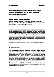
2.1. Multilayer Perceptron A multilayer perceptron [19] comprises several layers (typically two or three) of similar simple processing elements, called neurons, which take the previous layer’s neurons’ outputs as inputs, as illustrated in Figure 1. Each neuron computes a weighted sum of its inputs and modifies the result by means of a bounded non-linear activation function ϕ whose purpose is to limit the range of the neuron’s output. The transfer function for a neuron k is thus given by vk = bk +

∑w

jk

j

⋅oj

(1)

ok = ϕ (vk )

where the sum runs over all neuron inputs, and oj denotes the output of neuron j. The network’s free

International Journal On Advances in Systems and Measurements, vol 2 no 1, year 2009, http://www.iariajournals.org/systems_and_measurements/

46

Fix a training vector (xi , y i ) . Starting at the output neurons, a local gradient is calculated as δ j = ϕ ′(v j )⋅ ε j

(3)

where εj is the neuron’s error, i.e., the difference between the estimated output ϕ (v j ) and the desired output from the training vector. The local gradients in other layers are computed iteratively following the formula  

δ j = ϕ ′(v j )⋅ 

Fig. 1. A fully connected 2/5/4/1 multilayer perceptron. parameters are the weights wjk and biases bk in each neuron. The numbers of layers and of neurons in each layer are enough to completely describe the topology of a fully connected MLP, i.e., a network where all connections between neurons in consecutive layers are present. We shall use the notation N0 / N1 / … / NM to refer to a MLP with N0 inputs and M layers of neurons, where the i-th layer has Ni neurons. Partially connected MLPs can be thought of as special cases of MLP where some weights are forced to 0.

2.2. Backpropagation MLP training is the process of adaptation of the free parameters in such a way that the network’s global transfer function approaches some specific target behavior. This target function is defined by means of a set of V training vectors {(xi , y i )}Vi=1 , representing sample inputs xi and their associated desired network outputs yi. The set of network weights W is adjusted iteratively with the goal of minimizing the mean square error (MSE) 1 E (W ) = 2V

V

∑ F (x ; W ) − y i

2 i

(2)

i =1

where F is the ANN’s transfer function, dependent on the parameters W, and denotes the Euclidean norm in NM–dimensional space. In order to minimize E, computation of the gradient ∇E is needed. The most popular way to do this is the error backpropagation algorithm, or simply backpropagation [20], because of its efficient parallel, distributed implementation. This method of obtaining the network gradient consists of propagating neuron errors through the network layers in reverse order as follows:

∑w k

jk

 ⋅δk  

(4)

where the sum runs over all neurons k in the next layer. Finally, the gradient for weight wjk, connecting neuron/input j with neuron k in the next layer, is given by ∂E ∂w jk

= o j ⋅ δk

(5)

vector i

The gradient for the bias bk is equal to δk. Thus, the computations involved in the backpropagation algorithm for each training vector can be structured into three distinct phases (most authors only mention two phases; the last one is either ignored or merged with the second one): • Forward phase: The outputs (and derivatives) in each neuron are computed recursively, from the first to the last layer. • Backward phase: The local gradients δj in each neuron are computed recursively, backwards from the last to the first layer. • Gradient phase: Gradients for each free parameter are computed using (5). Computations for this phase can be organized in any order. Each individual phase may be carried out with parallel and distributed processing, however the forward and backward phases must be executed sequentially due to data dependence; failure to do so leads to a modified training algorithm [13]. The complete gradient for one epoch, i.e. presentation of the whole training set, is obtained by averaging the partial contributions from all training vectors: ∂E 1 = ∂w jk V

V

∂E

∑ ∂w i =1

jk vector i

.

(6)

International Journal On Advances in Systems and Measurements, vol 2 no 1, year 2009, http://www.iariajournals.org/systems_and_measurements/

47

-4

1

8

0.5

6

0

4

-0.5

2

-1 -8

-4

0

4

x 10

0 -8

8

Fig. 2. Hyperbolic tangent.

-4

0

ϕ (t ) =

One common approach to weight adjustment is MSE minimization by standard gradient descent, i.e. the weights are updated by subtracting a multiple of their respective gradients from them after each epoch:

(

)

8

Fig. 3. Approximation error for the modified activation function.

2.3. Resilient Propagation

W (n +1) = W (n ) − µ ⋅ ∇E W (n )

4

(7)

However, this procedure may provide very slow global network convergence due to a few neurons becoming saturated, i.e. having outputs close to the bounds given by the activation function and very small derivatives, leading to small weight updates between epochs, even if said weights are still far from their optimal values. A number of modifications of the weight update mechanism have been proposed in order to address this issue, including conjugate gradient algorithms [21] and quasi-Newton methods [22]. We have selected the Resilient Propagation (RPROP) algorithm [23], where the magnitude of each weight update is kept independent of the gradient; instead, the last weight update is stored as reference and amplified or reduced depending on whether the gradient maintained or changed its sign. RPROP is reportedly faster than gradient descent by an order of magnitude, and allows a very efficient hardware implementation, in terms of both execution time and resource occupation.

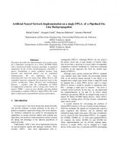
2.4. Activation Function It is a well-known fact that MLPs with at least two layers are universal approximators, i.e. they can be used to approximate any given continuous mapping with arbitrary accuracy on a bounded domain, as long as the activation function ϕ is bounded, monotone, and continuously differentiable [24]. Besides, convergence has been shown to be faster if ϕ is an odd bipolar function [25]. The most common activation function, shown in Figure 2, is the hyperbolic tangent

et − e −t et + e − t

(8)

which has all of the aforementioned properties. However, this function does not lend itself to an efficient digital implementation, requiring large operators to implement exponentials and division. Traditionally, ANN implementations have resorted to either look-up tables (LUT) or low-order approximations of ϕ, such as piecewise linear approximations [26], but these approaches are not viable in our situation: a LUT with floating-point precision would be too big, and piecewise linear approximations, while useful for hardware realizations of the recall phase of MLPs (i.e. of pre-trained networks with fixed weights), are inadequate for the implementation of the training phase, since they don’t satisfy the hypothesis of the universal approximation theorem, thus hurting network convergence. Our solution has been to implement a modified activation function ϕ~ , which is an odd cubic spline approximation of ϕ, with fixed exact values at abscissae 0, 0.25, 0.5, 1, 1.5, 2 and 3, saturation at 4, and fixed derivatives at the extreme points. This is a valid activation function since it satisfies all conditions stated previously, so it provides valid ANNs with correct training. This modified function allows an efficient implementation in our system architecture, based on repeated multiply-and-accumulate (MAC) operations. It can also be approximated by the hyperbolic tangent if needed, with an absolute error lower than 10–3, as shown in Figure 3.

3. System architecture description An overview of the designed system architecture and included components is presented in Figure 4. The core of the system is the neural coprocessor, with an embedded microcontroller acting as master processor,

International Journal On Advances in Systems and Measurements, vol 2 no 1, year 2009, http://www.iariajournals.org/systems_and_measurements/

48

Fig. 4. System architecture.

Fig. 5. Contents of the neural coprocessor. running from a program memory block which may be external to the FPGA. Input data flows to the coprocessor, i.e. training vectors and coprocessor instructions, are fed to the coprocessor input queues using DMA devices, controlled by the master processor. Memory blocks containing current network weights and resulting gradients are integrated into the coprocessor, but are also externally accessible. All coprocessor ports are implemented as Altera Avalon slave interfaces. An external training set repository is assumed, as well as memory blocks for the storage of the coprocessor subprogram and the variables of the RPROP algorithm (weight update magnitudes and previous network gradient). The two latter should be internal to the FPGA to increase performance.

3.1. Coprocessor architecture Figure 5 depicts the components of the neural coprocessor. It consists of a parameterized number P of arithmetic processing units (PU), restricted to a power of two to simplify logic design. All PUs execute the same operations simultaneously, and are capable of processing up to 8 different time-multiplexed data flows thanks to datapath pipelining. Each of the 8P supported data flows has an associated internal memory block for the storage of temporary variables; these memories can be individually read or written in order to set up the training session or retrieve results, according to an Active Data Flow Register.

International Journal On Advances in Systems and Measurements, vol 2 no 1, year 2009, http://www.iariajournals.org/systems_and_measurements/

49

Fig. 6. RTL description of a processing unit. The coprocessor’s control port allows the master processor to access internal control registers in order to modify the coprocessor’s behavior. Options include automatic endianness conversion for training vectors and results, to support communication with different remote hosts, and clearing of the gradient memory, in order to set up new training epochs. Additionally, a Valid Data Level Register specifies the number of data flows actually in use, so that results from invalid data flows may be ignored. Coprocessor status signals can also be read from the control port; they include input/output FIFO status and a “user bit” configurable through coprocessor instructions. These signals are used for execution flow control. Figure 6 shows the schematic for the contents of each PU. It consists of an adder unit, a multiplier unit, a local memory block and a reduced number of local registers. The adder and multiplier units are based on Altera 32-bit floating-point pipelined IP cores. Both of them implement an 8-stage pipeline and accept a new operation each clock cycle. Their inputs can be chosen from the local registers, their current outputs, and hardwired constants (1 for the multiplier and 0 for the adder) that allow them to behave as shift registers. The set of operand choices for both units has been kept small in order to reduce both the logic usage and the size of the instruction word; the backpropagation algorithm was analyzed in order to determine the smallest possible set of operand choices.

Arithmetic operators are not disabled during instructions that don’t need to use them; instead, they are used as shift registers by multiplying its current value by 1 or adding 0, respectively. This is necessary because a different functional unit might need to read their outputs in successive clock cycles, corresponding to different data flows, hence these outputs must change every clock cycle. A dual-port memory block (one read and one write port) is used as a large register bank to store variables for each data flow; the top 3 bits from each port’s address input are used to select the correct data flow. A previous analysis of the backpropagation algorithm revealed that one read and one write operation per cycle are enough except in some parts of the backward phase, where two reads may be needed; however, allowing them in a single clock cycle would require a triple port memory which would have to be implemented as two dual port memory blocks in parallel, thus halving the amount of memory available for each data flow. Each PU has three general-purpose local registers named L0, L1 and L2, implemented as 8-stage 32-bit shift registers. They are used as intermediate storage between large memories (global weight memory or local register banks) and the arithmetic units, in order to allow reuse of commonly accessed variables. Additionally, two registers C0 and C1 are used to load polynomial coefficients from a small 512 bit LUT, for the computation of the spline function ϕ~ and its

International Journal On Advances in Systems and Measurements, vol 2 no 1, year 2009, http://www.iariajournals.org/systems_and_measurements/

NEW ADFR VECTOR IN RESULT OUT

long inst.

L2 LOAD L1 SEL L1 LOAD L0 LOAD C LOAD

MUL SEL A

MUL SEL B

ADD SEL A

ADDER TREE STORE SEL STORE ADD SEL B

short inst. USER BIT SET USER BIT

50

Fig. 7. Coprocessor instruction word format. derivative; the value of the abscissa is always taken from L0. C0 is used for multiplicative and C1 for additive coefficients. As illustrated in Figure 6, the inputs to the adder subsystem in each PU can be bypassed using external control signals, allowing the coprocessor to rearrange the existing adder logic into a multistage adder tree, which can be used to combine results from different data flows.

3.2. Coprocessor programming model Figure 7 describes instruction word format for the neural coprocessor. There are two different types of instructions: “short” and “long” instructions, with a length of 32 and 64 bits respectively. The purpose of short instructions is to implement communication with the coprocessor’s input and output data streams by accessing individual addresses in local memory. Each instruction specifies up to three sequential tasks: updating the Active Data Flow Register, writing the contents of internal memory address A0 from the (new) active data flow into the output queue, and loading the first word from the FIFO vector queue into address A3. Additionally, the value of the “user bit” available through the control port may be changed. These instructions are consumed at a rate of one every clock cycle and implement a three stage instruction pipeline. Long instructions are used to perform arithmetic operations on values in local memory, possibly using weights from global memory as parameters. Each instruction specifies four different operations that are executed sequentially, if enabled: • Loading local registers with values from memory. Addresses A0 from local memory and A1 and A2 from global memory are available. Also, coefficient register C0 is loaded.

• Multiplication. Four bits are used to select input operands; a value of zero indicates “no operation”, i.e., multiplying the current output with 1. Register C1 is also loaded in this stage. • Addition. Again, four bits select the values to be added, with zeros indicating addition of the current adder output with 0. • Storing arithmetic results (from either the adder or the multiplier) into address A3 of local memory. This specifies four instruction pipeline stages, each one taking 8 clock cycles to complete. A new instruction is accepted every 8 clock cycles; each cycle, a new input is taken from a different data flow. Hence the coprocessor works as a Single-Instruction MultipleData (SIMD) machine, with the same instruction executing simultaneously on all PUs and acting on 8 time-multiplexed data flows within each PU. The execution of long instructions follows the VLIW (Very Long Instruction Word) paradigm, in that a sequence of simple sequential operations on the execution units (adder, multiplier, registers) is specified by a single instruction, so that instruction-level parallelism is achieved at compilation time. The coprocessor hardware provides no forwarding or scheduling logic; instead, the compiler that generates coprocessor code is responsible for the optimization of the algorithm and the prevention of data hazards between consecutive instructions with data dependence, inserting NOP instructions or ad-hoc data forwarding as needed. Thus, hardware complexity is reduced at the expense of increased compilation time. An extra bit in the instruction word allows the coprocessor to enter an extended instruction pipeline that implements an adder tree. Adder input selection is ignored in this case; instead, the bypass signals shown in Figure 6 are used to implement the accumulation of results from the multipliers in each data flow. Figure 8

International Journal On Advances in Systems and Measurements, vol 2 no 1, year 2009, http://www.iariajournals.org/systems_and_measurements/

51

schematizes the connections between multipliers and adders in both operating cases. The organization of the resulting adder tree into pipeline stages is shown in Figure 9. Accumulation of the outputs of the multipliers is divided in two different phases. The first phase uses P − 1 adders to implement a log 2 P -stage adder tree where spatial accumulation is performed, i.e., results from the same time slot in different PUs are combined. Its output is a stream of 8 partial sums coming out in consecutive clock cycles, which are accumulated in the second phase using the remaining adder and delay lines. There are eight available time slots; seven of them are used to combine of the partial sums using a 3-stage temporal tree structure, obtaining the sum of all multiplier outputs. The last time slot is used to accumulate that value with the previous value in address A2 of gradient memory. The second phase is independent of P and takes 5 eight-cycle stages to complete.

Fig. 8. Left: normal configuration. Right: Adder tree configuration.

4. System software This implementation of MLP training takes advantage of training-set parallelism, with different training vectors being handled in different coprocessor data flows using the same instructions. This obviously restricts our implementation to batch-mode training.

4.1. Backpropagation algorithm The coprocessor code necessary for ANN training is divided into two distinct sections. The first one is a series of short instructions that read values from the vector queue and store them in the correct local memory addresses for each data flow. This way, up to 8P whole training vectors are loaded into the same local addresses. The second section is formed by long (arithmetic) instructions that execute both the backpropagation algorithm and the gradient accumulation process. All data flows share the same local memory map, with their input values (training vectors) being pre-loaded by the first part of the program. An extensive analysis of the backpropagation algorithm has been done in order to achieve an optimal translation into coprocessor instructions, following the three phase structure described in Section 2.2. In the forward phase, the outputs and derivatives from all neurons in each layer are computed sequentially, according to (1). For each layer, the value of vk is obtained first for all neurons k in that layer, using as many MAC instructions as layer inputs for each neuron. The coprocessor ability to load two different network weights is exploited to include the

Fig. 9. Adder tree pipeline stages. addition of bias bk with no need for an extra instruction. After all vk have been computed, the activation function and its derivative are evaluated using the Horner scheme [27], organizing arithmetic operations as a sequence of n MACs, where n is the polynomial degree: ϕ~ (x ) = a3 x 3 + a2 x 2 + a1x + a0 = ((a3 ⋅ x + a2 ) ⋅ x + a1 ) ⋅ x + a0 ~ ′ ϕ (x ) = b2 x 2 + b1 x + b0

(9)

= (b2 ⋅ x + b1 ) ⋅ x + b0

Both polynomials can be computed in parallel by alternating the use of the adder and the multiplier, such that in a given 8-cycle stage, the adder is evaluating one of the functions while the multiplier is evaluating the other one. This is outlined in Figure 10, where each horizontal line represents concurrent operations. This

International Journal On Advances in Systems and Measurements, vol 2 no 1, year 2009, http://www.iariajournals.org/systems_and_measurements/

52

Fig. 10. Evaluation of the activation function and its derivative. way, only 5 instructions are necessary for the computation of the activation function and its derivative. The backward phase begins with simple multiplication operations to obtain local gradients in the output layer according to (3). For other layers, the bracketed sum in (4) needs to be computed first using as many MAC operations as neurons in the next layer; if the next layer is small enough, data forwarding has to be planned. Finally, the gradient phase makes use of the adder tree configuration of the coprocessor, computing gradients using (5) and then adding all multiplier results and accumulating them with the previous partial sum in gradient memory. Aggregated square error is also computed and accumulated; it must be divided by the total number of vectors afterwards to obtain the epoch’s MSE (2).

4.2. Master processor program Execution of whole training sessions is controlled by the master processor. The first action is initialization of network weights using the Nguyen-Widrow rule [28]; initial weights are then stored in the coprocessor’s weight memory. Afterwards, coprocessor code is compiled for both code sections specified in Section 4.1 and stored in memory; this code loads 8P vectors, executes backpropagation on all of them simultaneously and accumulates the results in gradient memory. Coprocessor code needs to be recompiled each time because it is dependent on network topology, which is a parameter for each training session. Arbitrary MLP topologies are supported, as long as each data flow’s local memory is large enough to contain all associated temporary variables.

After these initialization steps, the actual training is performed. New epochs are issued until a stop condition is fulfilled (either a maximum number of epochs is reached, or the network’s MSE falls below a given threshold). For the master processor, each epoch consists of a series of DMA transfers. A transfer of the whole training set into the vector queue is first set up. After that, a number of consecutive transfers of the whole coprocessor code into the instruction queue are issued, as many times as needed to exhaust the whole training set, since only 8P vectors are processed each time. Before the first transfer, the control port must be used to tell the coprocessor to overwrite gradient memory instead of accumulating previous results; this option must be turned off after the first iteration. Similarly, for the last transfer, the value of the Valid Data Level Register must be updated to reflect the actual number of vectors left, so that outputs from inactive data flows are not accumulated when computing gradients. After the last instruction transfer is processed, the gradient memory contains the final network gradient of (6), except for the factor 1 V , as well as the epoch’s aggregated square error. The RPROP algorithm is now executed by the master processor to obtain the new network gradients; the multiplicative factor 1 V is irrelevant since only the sign of the gradient components is used.

5. Implementation The system has been implemented on an Altera DE2-70 development board, with a Cyclone II EP2C70F896C6 reconfigurable device and external RAM memory for both the master processor program and storage of the training set; up to 64 MB are available for training vectors. The master controller is implemented as a Nios II/f embedded processor. A 16 KB internal memory for coprocessor instructions is necessary to contain the program for all applicable MLP topologies. The limitation on the size of the coprocessor fitting into the FPGA comes from the amount of available onchip memory blocks for the realization of local memories, hence the minimum amount of necessary memory was determined first. It was established that 128 words (4 kbit) were enough for each data flow, allowing the training of networks with up to approximately 40 neurons. Also, weight and gradient memories were limited to 2 KB, imposing a limit of 511 network weights. Each coprocessor PU has an occupation of approximately 2970 logic elements and 10 4-kbit memory blocks, as well as four 18x18 multiplier

International Journal On Advances in Systems and Measurements, vol 2 no 1, year 2009, http://www.iariajournals.org/systems_and_measurements/

53

6. Performance Training performance was evaluated for the wellknown Iris plants problem [29], using a data set consisting of 150 four-dimensional inputs and three different outputs representing membership to three different classes with the values 1 and –1. The number of training epochs was fixed to 100, and the size of the training set V was modified by replicating the base data set. The number of CUPS (Connection Updates Per Second) was selected as a metric for system performance. This quantity is defined as the amount of network parameters divided by the time needed to process each training sample and update network parameters accordingly; for batch training, this is equal to CUPS =

WVN epochs WV = Tepoch Ttraining

(10)

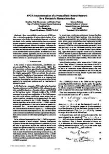
where W is the number of network weights, Nepochs is the number of training epochs, and Tepoch and Ttraining are the time length of each epoch and the whole training session, respectively. The largest topology supported by the system for the Iris problem was found to be the 4/18/18/3 MLP. Training time was measured for this network and the smaller 4/5/5/3, 4/9/8/3 and 4/12/12/3 topologies.

500 Performance (MCUPS)

blocks, with full-capability floating-point operators, i.e. supporting denormal numbers and full-range rounding. It is possible to fit up to P = 16 processing units in the coprocessor for this FPGA, allowing the simultaneous processing of up to 128 training vectors. The coprocessor works with an internal 100 MHz clock, while the rest of the system uses a 50 MHz clock; the use of dual-port memories for every coprocessor interface makes it possible to implement independent clock domains. Thus, the coprocessor has a maximal computational performance of 3.2 GFLOPS; this value is maintained during most of the execution of the backpropagation algorithm and gradient accumulation. The system makes use of the on-board Ethernet NIC to allow the board to be connected to a local IP network, so that a remote computer can use the FPGA system to perform any network training. The remote host needs to provide the MLP topology, the whole training set, and training stop conditions (maximum epoch number or MSE threshold). On training completion, the board returns the final network weights, the MSE evolution for all epochs, and information about total training time. Matlab has been used to implement the connection protocol and test the training results on the client PC side.

400 300 200 4/5/5/3 4/9/8/3 4/12/12/3 4/18/18/3

100 0 2 10

10

3

4

10 Training vectors

10

5

Fig. 11. System performance for different topologies and training set sizes. Results are plotted in Figure 11. Training performance increases approaching a limit value as the training set grows larger, as expected from a system where parallelization speedup stems primarily from training set parallelism; this limit value is dependent on network topology. Since vector loading time is constant for a given problem, the fraction of execution time spent on arithmetic computations (backpropagation and gradient accumulation) is higher for more complex topologies. Hence, system performance increases as the MLP size grows, converging to a peak value for sufficiently complex networks (4/12/12/3 and higher). For our implementation, this peak value is 431 MCUPS.

7. Conclusion and future work A system-on-chip architecture for MLP training has been proposed, where a high level processor controls the system execution flow and data transfers and generates parameterized machine code, depending on network topology, for a low level custom hardware coprocessor where the backpropagation algorithm is carried out. A SIMD architecture for the neural coprocessor is described, with a large number of replicated pipelined arithmetic operators in order to support the simultaneous processing of hundreds of training vectors. Optimized coprocessor code allows the arithmetic operators to reach near 100% utilization. Implementation of the proposed architecture on a low-cost Altera FPGA reaches a training performance exceeding 430 MCUPS. This is a competitive value compared to other state-of-the-art FPGA implementations of MLP training with fixed topology and fixed point precision. As far as we know, no other FPGA implementation exists with floating point precision and arbitrary topology training without device reconfiguration; such features are exclusive of either software implementations on general-purpose

International Journal On Advances in Systems and Measurements, vol 2 no 1, year 2009, http://www.iariajournals.org/systems_and_measurements/

54

processors, which are slower, or ASIC implementations (so-called neurochips), which are much more costly. Scalability of this architecture on larger FPGAs is constrained mainly by the amount of available on-chip memory for the realization of local memory blocks; it is probably not practical to relocate this resource to external memory because of frequent, wide access (512 bits every clock cycle for our current implementation). The addition of custom superpipelined floating-point operators might allow higher clock frequencies, although they will be ultimately be limited by FPGA routing resources. We intend to explore the possibility of using floating-point representations with less than 32 bits, as well as the adaptation of the neural coprocessor architecture to allow other types of ANN such as Radial Basis Networks.

Acknowledgments This work was supported by the Spanish Ministry of Science and Innovation under FPU Grant AP200604275 and the Education Department of the Valencian Government under Grant GVPRE/2008/082.

References

[7] R. P. Lippmann, “Review of neural networks for speech recognition”, Neural Computation, no. 1, pp. 1-38, 1989. [8] R. J. Aliaga, J. D. Martinez, R. Gadea, A. Sebastiá, J. M. Benlloch, F. Sánchez, N. Pavón and C. W. Lerche, “Corrected position estimation in PET detector modules with multi-anode PMTs using neural networks”, IEEE Transactions on Nuclear Science, vol. 53, no. 3, pp. 776-783, 2006. [9] D. K. McNeill, C. R. Schneider and H. C. Card, “Analog CMOS neural networks based on Gilbert multipliers with incircuit learning”, Proceedings of the 36th Midwest Symposium on Circuits and Systems, vol. 2, pp. 1271-1274, 1993. [10] T. Theocharides, G. Link, N. Vijaykrishnan, M. J. Irwin and V. Srikantam, “A generic reconfigurable neural network architecture as a network on chip”, Proceedings of the IEEE International SoC Conference, pp. 191-194, 2004. [11] J. L. Holt and T. E. Baker, “Backpropagation simulations using limited precision calculations”, Proceedings of the International Joint Conference on Neural Networks, vol. 2, pp. 121-126, 1991. [12] A. W. Savich, M. Moussa, and S. Areibi, “The impact of arithmetic representation on implementing MLP-BP on FPGAs: A study”, IEEE Transactions on Neural Networks, vol. 18, no. 1, pp. 240-252, 2007.

[1] R. J. Aliaga, R. Gadea, R. J. Colom, J. M. Monzó, C. W. Lerche, J. D. Martinez, A. Sebastiá, F. Mateo, “Multiprocessor SoC implementation of neural network training on FPGA”, 2008 International Conference on Advances in Electronics and Micro-electronics (ENICS), pp. 149-154, 2008.

[13] R. Gadea, J. Cerdá. F. Ballester, and A. Mocholí, “Artificial neural network implementation on a single FPGA of a pipelined on-line backpropagation”, Proceedings of the 13th International Symposium on System Synthesis, pp. 225230, 2000.

[2] W. S. McCulloch and W. H. Pitts, “A logical calculus of the ideas imminent in nervous activity”, Bulletin of Mathematical Biophysics, no. 5, pp. 115-133, 1943.

[14] C. Xiang, S. Q. Ding and T. H. Lee, “Architecture analysis of MLP by geometrical interpretation”, 2004 International Conference on Communications, Circuits and Systems, vol. 2, pp. 1042-1046, 2004.

[3] B. Widrow and M. E. Hoff, “Adaptive switching circuits”, IRE WESCON Convention Record, part 4, pp. 96104, 1960. [4] J. Zhu and P. Sutton, “FPGA implementations of neural networks – a survey of a decade of progress”, Proceedings of the International Conference on Field Programmable Logic, pp. 1062-1066, 2003. [5] M. R. Zargham, Computer Architecture: Single and Parallel Systems, p. 346, Prentice Hall, 1996. [6] N. L. D. Khoa, K. Sakakibara, and I. Nishikawa, “Stock price forecasting using backpropagation neural networks with time and profit based adjusted weight factors”, Proceedings of the SICE-ICASE International Joint Conference, pp. 54845488, 2006.

[15] B. Hassibi, D. G. Stork and G. J. Wolff, “Optimal Brain Surgeon and general network pruning”, Proceedings of the International Conference on Neural Networks, vol. 1, pp. 293-299, 1993. [16] G. F. Miller, P. M. Todd and S. U. Hedge, “Designing neural networks using genetic algorithms”, Proceedings of the 3rd International Conference on Genetic Algorithms, pp. 379-384, 1989. [17] X. Yao, “Evolutionary artificial neural networks”, International Journal of Neural Systems, vol. 4, no. 3, pp. 203-222, 1993. [18] S. Babii, V. Cretu, and E. Petriu, “Performance evaluation of two distributed backpropagation implementations”, Proceedings of the International Joint Conference on Neural Networks, Orlando, 2007.

International Journal On Advances in Systems and Measurements, vol 2 no 1, year 2009, http://www.iariajournals.org/systems_and_measurements/

55

[19] S. Haykin, Neural Networks: A Comprehensive Foundation, 2nd Edition, pp. 156-255, Prentice Hall, 1999. [20] D. E. Rumelhart, G. E. Hinton and R. J. Williams, “Learning internal representations by error propagation”, Parallel Distributed Processing: Explorations in the Microstructures of Cognition, Vol I: Foundations, Chapter 8, MIT Press, Cambridge, Massachusetts, 1986. [21] C. Charalambous, “Conjugate gradient algorithm for efficient training of artificial neural networks”, IEE Proceedings – Circuits, Devices and Systems, vol. 139, no. 3, pp. 301-310, 1992. [22] R. Fletcher, Practical Methods of Optimization, 2nd Edition, pp. 49-57, John Wiley & Sons, 1987. [23] M. Riedmiller and M. Braun, “A direct adaptive method for faster backpropagation learning: the RPROP algorithm”, Proceedings of the IEEE International Conference on Neural Networks, vol. 1, pp. 586-591, 1993. [24] K. Hornik, M. Stinchcombe and H. White, “Multilayer feedforward networks are universal approximators”, Neural Networks, vol. 2, pp. 359-366, 1989. [25] Y. Le Cun, I. Kanter and S. A. Solla, “Second order properties of error surfaces: learning time and generalization”, Proceedings of the Conference on Advances in Neural Information Processing Systems, vol. 3, pp. 918-924, 1990. [26] V. Havel and K. Vlcek, “Computation of a nonlinear squashing function in digiral neural networks”, 11th IEEE Workshop on Design and Diagnostics of Electronic Circuits and Systems, pp. 1-4, 2008. [27] D. Knuth, The Art of Computer Programming, vol. 2: Seminumerical Algorithms, 3rd Edition, pp. 486-487, Addison-Wesley, 1997. [28] D. Nguyen and B. Widrow, “Improving the learning speed of 2-layer neural networks by choosing initial values of the adaptive weights”, Proceedings of the International Joint Conference on Neural Networks, vol. 3, pp. 21-26, 1990. [29] R. A. Fisher, “The use of multiple measurements in taxonomic problems”, Annals Eugenics, pp. 179-188, vol. 7, 1936.