Target Detection with Improved Image Texture Feature ... - CiteSeerX

INTERNATIONAL JOURNAL OF INTELLIGENT TECHNOLOGY VOLUME 1 NUMBER 1 2006 ISSN 1305-6417

Target Detection with Improved Image Texture Feature Coding Method and Support Vector Machine R. Xu, X. Zhao, X. Li, C. Kwan, and C.-I Chang All texture-based methods can be roughly classified into two categories: structural-based approach and statistical-based approach. In recent years, the statistical-based approach is attracting more research interests [5]-[12]. In current statistical-based methods, Texture Feature Coding Method (TFCM) is a new texture analysis scheme which transforms an original image into a texture feature image whose pixel values represent the texture information of the pixel in original image. The method has several remarkable advantages including accurate representation and record of target texture, and computational efficiency [11], [12]. For pattern training and target detection, Support Vector Machine (SVM) is a powerful tool to use, which is originated from modern statistical learning theory [13]. SVM is a kernel-based learning algorithm and relies on the borderline training samples to define the separation hyperplanes. Its performance is better than most other learning algorithms for a wide range of applications including automatic target recognition, image retrieval, and document analysis. In this paper, we combine the TFCM-based feature extractors and the SVM-based pattern classifier into a unified package for ATR. With this proposed ATR system, the targets of interest in an input image can be efficiently detected. There are several distinctive advantages of this algorithm. First, a new target detection architecture (Texture feature extraction + SVM) is proposed, which combines the advantages of both TFCM and SVM. Second, the texture feature coding scheme in [12] is simplified to improve the computational efficiency. Third, two new TFCM-based feature extractors are developed. One is based on the principal eigenvector of the co-occurrence matrix of the texture feature numbers (TFN) and the other one is an augmented and much more efficient version of the one given in [12]. For the purpose of comparison, the texture feature number (TFN) histogram method for feature extraction [12] is also implemented. Fourth, with the extracted features, a robust and computationally efficient pattern classifier based on SVM is then trained and used for target detection. Fifth, a new technique called Cascade Sliding Window (CSW) is developed to perform automated target localization. We have applied and evaluated the proposed ATR framework to different real life scenarios (different data sources), including mammogram, Synthetic Aperture Radar (SAR), and Ground Penetrating Radar (GPR) images. The rest of this paper is arranged as follows. Section 2 summarizes all the technical methods, including the TFCM

Abstract—An image texture analysis and target recognition approach of using an improved image texture feature coding method (TFCM) and Support Vector Machine (SVM) for target detection is presented. With our proposed target detection framework, targets of interest can be detected accurately. Cascade-Sliding-Window technique was also developed for automated target localization. Application to mammogram showed that over 88% of normal mammograms and 80% of abnormal mammograms can be correctly identified. The approach was also successfully applied to Synthetic Aperture Radar (SAR) and Ground Penetrating Radar (GPR) images for target detection. Keywords—Image texture analysis, Feature extraction, Target detection, Pattern classification

A

I. INTRODUCTION

UTOMATIC Target Recognition (ATR) has many applications. One typical application is target detection in battlefield, such as the detection of moving people and vehicle, land mines, and weapon concealment. Besides military applications, one important objective of computeraided medical diagnosis in medical practices is to correctly detect anomalies in medical images such as mammogram, computer tomography, and magnetic resonance imaging. A general image analysis-based ATR framework consists of target feature extraction, target pattern training, and target detection. Among them, feature extraction is considered as a very important part. Many research efforts have been conducted in this area in recent years, especially for target feature extraction by using image texture analysis [1]-[4] for target feature extraction as it has been observed that target textures are different from cluttered surroundings, which means target texture can help a lot on target detection.

Manuscript received April 18, 2006. This work was supported by the U.S. Navy under Grant N68335-03-C-0034. R. Xu is with Intelligent Automation Inc., Rockville, MD 20855 USA (phone: 301-294-5200; fax: 301-294-5201; e-mail: hgxu@ i-a-i.com). X. Zhao, X. Li, and C. Kwan are with Intelligent Automation Inc., Rockville, MD 20855 USA C.-I Chang is with the Remote Sensing Signal and Image Processing Laboratory, Department of Computer Science and Electrical Engineering, University of Maryland Baltimore County, Baltimore, MD 21250 USA.

IJIT VOLUME 1 NUMBER 1 2006 ISSN 1305-6417

47

© 2006 WASET.ORG

INTERNATIONAL JOURNAL OF INTELLIGENT TECHNOLOGY VOLUME 1 NUMBER 1 2006 ISSN 1305-6417

(iii) I (a) − I (b) > ∆, I (b) − I (c) > ∆ or

concept, three feature extractors (feature descriptors, TFN histogram, and principal eigenvector of the texture feature cooccurrence matrix), SVM classification method, and the CSW method for automatic target localization. Experimental results in mammograms, SAR images, and GPR images, are reported in Section 3 to demonstrate the efficiency of our proposed approach. Concluding remarks are given in Section 4.

I (b) − I (a) > ∆, I (c) − I (b) > ∆

(iv) I (a ) − I (b) > ∆, I (c) − I (b) > ∆ or I (b) − I (a) > ∆, I (b) − I (c) > ∆

II. ALGORITHM DESCRIPTION A. Texture Feature Coding Method (TFCM) For target detection in cluttered and complex environment, texture feature is considered as the major or only possible feature for target detection. Among the texture-based methods, texture feature coding method is well known for its efficiency. The concept of the TFCM [12] is derived from the gray-level co-occurrence matrix [14] and texture spectrum method [15]. In our proposed ATR approach, a simplified version of TFCM is developed to save more computation time. For better understanding, some key concepts of TFCM are briefly described as follows. Fig. 1(a) shows a 3x3 window mask over a pixel, in which there are eight orientations, 0o, 45o, 90o, 135o, 180o, 225o, 270o, and 315o. Fig. 1(b) shows a 4-neighbor connectivity of a pixel X with four pixels labeled as 1, 3, 5, and 7 which are referred as first-order neighboring pixels. The additional four pixels labeled as 2, 4, 6, and 8, and located along two diagonal lines are referred as second-order neighboring pixels as shown in Fig. 1(c).

Fig. 2 Types of gray-level graphical structure variations

If we introduce a pair of integers (v, w) to represent the gray-level variations of first-order and the second-order connectivity respectively, and consider the symmetry between first scan line and second scan line of first-order or second order connectivity, the number of each connectivity combinations can be reduced to 4*(4+1)/2=10, as shown in Table 1. In the conventional method [12], Table 1 is coded in a discrete way from 1 to 23 according to the definition given in [15]. Then, for the pair of integers (v, w) of any image pixel, its texture feature number (TFN) can be computed as TFN ( x, y ) . (2) TFN ( x, y ) = α ( x, y ) × β ( x, y ) where α ( x, y ) and β ( x, y ) are the values obtained from Table 1. According to Eq. (2), the number range is from 1 to 529, but only 55 are actually used for texture feature coding. Therefore, to save computational cost and memory space, we compress the set of 1 to 529 to 0 to 54 values by removing unused texture feature numbers. TABLE I COMBINATION CODING OF THE GRAY-LEVEL VARIATIONS (I) First scan line Second scan line

Fig. 1 First-order and second-order 4-neighbor connectivity

(ii)

(iii)

(i)

1

2

3

(iv) 5

(ii)

2

7

11

13

(iii)

3

11

17

19

(iv)

5

13

19

23

Unlike the coding scheme mentioned above, we use continuous numbers to code the cases shown in Table 2. With the new table, for each gray-level variation (v, w) of an image pixel we can directly compute the TFNs, which are listed in Table 3. If we ignore the difference between the first order and the second order connectivity, we can find the texture feature number TFN ∆ ( x, y ) , of the pixel at location (x,y)

TFCM considers three consecutive pixels along these specific directions (called scan lines), and calculates gradient changes in gray levels among these three pixels [12]. We denote the three consecutive pixels by their spatial coordinates at a, b, c, associate its gray level by I(a), I(b) and I(c) respectively, and let ∆ be a desired gray level tolerance. There are four types of successive gradient changes in gray level with their corresponding graphic descriptions given in Fig. 2. (i) | I (a) − I (b) |≤ ∆, | I (b) − I (c) |≤ ∆ (ii) | I (a ) − I (b) |≤ ∆, | I (b) − I (c) |> ∆ or (1) | I (a) − I (b) |> ∆, | I (b) − I (c) |≤ ∆

IJIT VOLUME 1 NUMBER 1 2006 ISSN 1305-6417

(i)

according to Table 3. In this way, the computation time of (a,b) is greatly reduced. That is, a simple table look-up is enough to generate the TFNs.

48

© 2006 WASET.ORG

INTERNATIONAL JOURNAL OF INTELLIGENT TECHNOLOGY VOLUME 1 NUMBER 1 2006 ISSN 1305-6417

B. Texture Feature Extraction Based on the TFN histogram and TFCM-based Cooccurrence matrix, two new feature extractors were developed. One is named as eigenvector-based feature extraction and another one called statistical analysis-based method is an augmented and more computationally efficient version of the one given in [12]. For comparison, one traditional feature extractor, called TFN histogram, was also implemented. All the details are discussed as follows.

TABLE II COMBINATION CODING OF THE GRAY-LEVEL VARIATIONS (II) First scan line Second scan line

(i)

(ii)

(iii)

(iv)

(i)

1

2

3

4

(ii)

2

5

6

7

(iii)

3

6

8

9

(iv)

4

7

9

10

•

TFN histogram The TFN histogram introduced by [12] has 55 dimensions to each image or region of interest, and can be used directly as feature descriptors independently as it contains rich texture information of the image or the region of interest. The definition of TFN histogram is given in Eq. (3). An example of TFN histogram on a mammogram image is given in Fig. 3.

TABLE III TEXTURE FEATURE NUMBER GENERATION TABLE BASED ON THE NEW CODING SCHEME 1 2 3 4 5 6 7 8 9 10

1 0 1 2 3 4 5 6 7 8 9

2 1 10 11 12 13 14 15 16 17 18

3 2 11 19 20 21 22 23 24 25 26

4 3 12 20 27 28 29 30 31 32 33

5 4 13 21 28 34 35 36 37 38 39

6 5 14 22 29 35 40 41 42 43 44

7 6 15 23 30 36 41 45 46 47 48

8 7 16 24 31 37 42 46 49 50 51

9 8 17 25 32 38 43 47 50 52 53

10 9 18 26 33 39 44 48 51 53 54

It is worth to mention that our new coding scheme has three unique properties. First, the TFN ∆ ( x, y ) is quasi-rotation(a) Original image

invariant because symmetry is considered during coding. Second, since TFN ∆ ( x, y ) only takes a value ranging from 0 to 54, the calculation of a TFCM based co-occurrence matrix of an image and some of its corresponding TFCM features will take less time. Third, the code value at a given pixel represents the coarseness of its neighborhood. The higher the code value is, the more gray-level variation its corresponding pixel possesses. All the aforementioned properties are very important as they capture the essence of the texture around a specific pixel. Once a TFN feature image is obtained by TFCM, two measures based on TFN histogram and TFCM-based Cooccurrence matrix, can be computed and used to characterize its statistics. A TFN histogram is defined as pTFN ,∆ (n) =

∑

(c) TFN histogram Fig. 3 TFN histogram of a mammogram image

•

Statistical Texture Feature Descriptors In order to capture the essence of texture information of an image, a set of texture feature descriptors was developed to represent the kernel texture information of the image or the region of interest. Here we introduce eleven descriptors. Some of them (1 to 8) were already discussed in [12], [16], the other three (9-11) are specially designed by us. The first two feature descriptors are derived from the TFN histogram of an image.

NTFN ,∆ (n) 54

NTFN ,∆ ( n)

(3) where NTFN .∆ (n) is the total number of TFN ∆ ( x, y ) in the image taking value n, and ∆ is the gray-level variation tolerance given in Eq. (1). The TFN based co-occurrence matrix, which is a probability distribution of transitions between any pair of arbitrary two TFNs, can be defined as N ∆ ,d ,θ (i, j ) (4) p∆ (i, j | d , θ ) = ∑ l ,k N ∆,d ,θ (l, k ) n=0

(b) TFN feature image

1. Mean convergence 54

MC = ∑

where N ∆ , d ,θ (i, j ) is the number of pairs of two pixels at

n =0

n ⋅ p ∆ ( n) − µ ∆

(5)

σ∆

where µ ∆ , σ ∆ are the mean and variance of the histogram, respectively. p∆ is defined in Eq. (4). 2. Code variance

spatial locations (x, y) and (w, z) satisfying TFN code level I(x,y) = i, I(w,z) =j and d-pixel apart along angular rotation θ and ∑ N ∆ , d ,θ (l , k ) is the total number of TFN transitions. l ,k

54

Var = ∑ (n − µ ∆ ) ⋅p ∆ (n) 2

n =0

IJIT VOLUME 1 NUMBER 1 2006 ISSN 1305-6417

49

© 2006 WASET.ORG

(6)

INTERNATIONAL JOURNAL OF INTELLIGENT TECHNOLOGY VOLUME 1 NUMBER 1 2006 ISSN 1305-6417

The remaining feature descriptors are based on the TFN cooccurrence matrix. Here we fix d = 1 and use the average of four matrices (corresponding to θ = 0 , θ = 45o , θ = 90o and θ = 135o ). That is,

Fig. 4 Summation regions of different subband probabilities. As a result of the above operators, each image or the region of interest in the database can be represented by an 11 x 1 feature vector. Since some features usually have large magnitudes and the others have small magnitudes, we scale different feature elements such that each feature contributes equally to the classifier

1 P∆,d = P(d =1,θ = 00 ) + P(d =1,θ = 450 ) + P(d =1,θ = 900 ) + P(d =1,θ =1350 ) 4

(

)

where P(d , θ ) is the TFN co-occurrence matrix with respect to d and θ . Based on P∆ ,d , we define the following features

•

Principal eigenvector of the TFN based co-occurrence matrix The 55x55 TFN co-occurrence matrix called P can be computed via Eq. (4) to an image or the region of interest. After performing eigenvalue decomposition on R= PPT , we found that, in most cases, the largest eigenvalue of R is larger than 85% of the sum of all the other eigenvalues of R. This means the 55 dimensional principal eigenvector of a TFN cooccurrence matrix, corresponding to its largest eigenvalue, may also well represent the texture properties of the image. It can either be feature vector independently or combined with the histogram feature vector. In one of our studies, we cascade the TFN histogram vector and the principal eigenvector to form a new 110 dimensional feature vector. With this newly developed feature set, we can achieve a good classification result in some conditions (See Section 3), which has, in return, validated our reasoning logic.

3. Code entropy 54

54

(7)

CE = ∑∑ p ∆ ,d (i, j ) log p ∆ ,d (i, j ) i =0 j = 0

4. Uniformity 54

54

(8)

UN = ∑∑ p ∆2 ,d (i, j ) i =0 j =0

5. First-order element difference moment (FDM) 54

54

(9)

FDM = ∑ ∑ i − j p ∆ ,d (i, j ) i =0 j =0

6. Second-order element difference moment (SDM) 54

54

(10)

SDM = ∑∑ (i − j ) 2 p ∆ ,d (i, j ) i =0 j =0

7. First-order inverse element difference moment (FIDM) 1 p∆,d (i, j ) 1 i− j + j =0

54 54

(11)

FIDM = ∑∑ i =0

8. Second-order inverse element difference moment (SIDM) 54

54

SIDM = ∑∑ i =0 j =0

1 p ∆ ,d (i, j ) 1 + (i − j ) 2

(12)

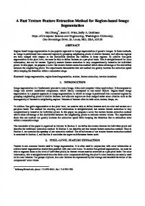
C. Support Vector Machine (SVM) for Classification According to the references [17], [18], SVM parameters are computed by solving a quadratic programming problem with linear equality and inequality constraints; rather than by solving a non-convex, unconstrained optimization problem. The flexibility of kernel functions allows the SVM to search a wide variety of hypothesis spaces. The geometrical interpretation of support vector classification can be thought as the optimal separation on feature surface. A simple example of 2-D data classification with three different classes using SVM is shown in Fig. 5, wherein the optimal boundaries are found between each pair of classes. The advantages of SVM include:

The following three features are the region-based features of the co-occurrence matrix.

9. to 11. Energy Distributions of Co-occurrence Matrix 54

54

(13)

SB1 = ∑ ∑ p ∆ ,d (i, j ) i = 44 j = 44

54

54

(14)

SB 2 = ∑ ∑ p ∆ ,d (i, j ) − SB1 i = 34 j =34

54

54

(15)

SB3 = ∑ ∑ p ∆ ,d (i, j ) − SB1 − SB 2

•

i =14 j =14

The summation regions (SB1, SB2, and SB3) are depicted in Fig. 4. In this way, the energy distributions of texture for different regions are being considered and added into the feature vector. Compared with the feature vector without energy distribution component, the feature vector with energy distribution can provide an additional 5% -10% increase in target recognition rate according to our tests.

• •

54

0

•

0

14

SB3 SB2 SB1 54

14

•

34 44

It is a quadratic learning algorithm; hence, there are no local optima. It can also be formed as linear programming for simplicity. Statistical theory gives bounds on the expected performance of a support machine. Performance is better than most other learning algorithms for a wide range of applications including automatic target recognition, and document classification Although originally designed for 2-class classification, SVMs have been effectively extended to multi-class classification applications. Algorithms, such as One-against-one, DAG, one-against-all, and C&S, have been successfully applied to multi-target recognition. There is no over-training problem as compared to conventional learning classifiers such as neural net or fuzzy logic.

34

IJIT VOLUME 1 NUMBER 1 2006 ISSN 1305-6417

50

© 2006 WASET.ORG

INTERNATIONAL JOURNAL OF INTELLIGENT TECHNOLOGY VOLUME 1 NUMBER 1 2006 ISSN 1305-6417

Image of interest

NxN Window segmented normal image

Cascade sliding window of size NxN segmentation

TFN histogram and eigen-vector feature extraction

TFN histogram and TFCM eigen-vector feature vector extraction

Fig. 5 SVM classification results of three classes

N N Image done?

Testing

The TFCM-SVM training and testing procedures based on the statistical feature descriptors are briefly summarized below: 1. Prepare M training images with known ground truth, which means we have already known which image is background image and which image is target image and the target type. Associate each image with an integer class label, for example, 0, 1, 2, …, M. 2. Perform TFCM on each image to obtain a feature image with its element being TFN numbers. 3. Calculate a TFN histogram for each feature image. 4. Calculate a TFCM co-occurrence matrix for the same feature image 5. Calculate the 11 texture feature descriptors using Eqs. (5) to (15) to represent the image being processed 6. Form all the image feature vectors into a 11xM matrix, regarded as the input matrix. Align their class labels to a 1xM row output vector. 7. Use the input and output pair to train the SVM. The result is stored in a set of vectors and matrices. In the testing stage, the first six steps are still applicable to a testing image. Compared with the training stage the difference is the trained support vector machine is used to output a label vector for a testing image at the last step (Step 7). Note that the TFCM-SVM procedures, either based on TFN histogram or principal eigenvector, have the similar steps as statistical feature descriptor-based method.

Classification parameters

Training

A

Mark the windowed image with the white frame

End

Fig. 6 Flow chart of the TFCM-SVM-CSW algorithm III.

EXPERIMENTAL RESULTS

A. Mammogram Inspection Our first case study was focused on mammogram inspection by using TFCM-SVM method. The database is the MiniMammographic Database provided by the Mammographic Image Analysis Society (MIAS). In our study, 59 normal mammogram images and 55 abnormal images containing different abnormalities were segmented from the database (totally 114 images). The abnormal regions were classified into the following 5 abnormal categories: • 13 in architectural distortions (ARCH), • 10 in asymmetry tissues (ASYM), • 12 in circumscribed masses (CRIC), • 11 in speculate masses (SPEC), • 9 in other/ill-defined masses (MISC). In our tests, we ran the TFCM method first to some randomly selected images from the above five categories as shown in Fig. 7, and some selected normal images as shown in Fig. 8. All normal images are 128x128 in size whereas the image size for the abnormal images varies as the area of the abnormal region differs from one case to another. After obtaining the features of all selected images, we used SVM with RBF (Radial Basis Functions) kernel to perform target classification. The cross validation method, also known as leave-one-out scheme, was used for training and testing. In this method, the decision rule is first obtained by using all but one of the samples in the data set, and the sample which is left out is then used to test the performance of the decision rule. This procedure is repeated for all the samples in the data set. For example, if there are I normal data and K abnormal data, then I+K classification results can be obtained by this method. From these we can obtain an estimate of the overall accuracy of the classification scheme. The results of our tests were summarized in from Table 4. It can be seen that the TFCMSVM with eigenvector has the best performance. Note that the leave-one-out is only suitable for off-line training and testing. The result by using CSW to a large image (1024x1024) which contains multiple abnormal regions is given in Fig. 9 to demonstrate the efficiency of our approach on automatic

D. Automatic Target Localization and Detection In order to localize and detect a target automatically, a Cascade Sliding Window (CSW) technique was developed. The key idea of the technique is to segment the whole image by a N × N pixel window and train the TFCM-SVM by using both the background/normal regions and the target regions. N is a predetermined value. In our experiments, the value of N is twice the size of the possible targets. To test a new image, the N × N pixel window moves around the image and feeds the segmented image into the TFCM_SVM for classification. The flowchart diagram of CSW is illustrated in Fig. 6.

IJIT VOLUME 1 NUMBER 1 2006 ISSN 1305-6417

Y

TFCM vector

SVM classifier training

SVM classification

Normal/Abnormal?

NxN Window segmented abnormal image

51

© 2006 WASET.ORG

INTERNATIONAL JOURNAL OF INTELLIGENT TECHNOLOGY VOLUME 1 NUMBER 1 2006 ISSN 1305-6417

classification performance of normal data is slightly reduced, the performance on abnormal data is improved, and the overall correct classification rate increases to 87%.

target detection and classification in online stage, wherein the yellow ellipsis is known as ground truth and the red rectangles are the detected targets. The performance of SVM is affected by two parameters, namely the kernel parameter γ and the regularization parameter C . For a given regularization parameter C , larger kernel parameter γ leads to smaller training error. The tradeoff is the generalization capability of the SVM will be reduced. If γ becomes too small, the two classes would be too close to each other, and the performance will also be degraded. In short, there is an optimal combination of the two SVM parameters, which can be obtained through trial-anderror. Some studies on parameter tuning with feature descriptor-based TFCM-SVM method are given in Table 5 and Table 6. In Table 5, we fixed C as 100, and showed the results with γ = 10−3 , γ = 10−4 , and γ = 10−5 , respectively. The cross validation method was used in the training and test. It can be seen that the best classification result was obtained with γ = 10−4 . In this case, the algorithm yields 90% correct detection for normal data and 80% correct classification for abnormal data. The overall correct detection rate is 85%. We then fixed γ as γ = 10−4 and varied the value of C to repeat the test. The results are shown in Table 6, in which the best performance is obtained at C = 10 4 and γ = 10−4 . Although the

CRIC (001)

ASYM (097)

B. Target Detection in Airborne SAR Images In this study, we applied the TFCM-SVM method to SAR images for target detection. The image we used is shown in Fig. 10. The unclassified raw image (size 765x765) was supplied by the U.S. Army. The image shown in Fig. 10 is filtered by a 5x5 median filter [4] to eliminate some noise spikes. A median filter is a rank filter which, for a given vector of data points, first sorts the points from smallest to largest, and then picks the median value as the filter output. We selected 9 regions of background and 10 regions of target in the experiment. Each region has a size of 64 x 64 pixels. These chosen regions are shown in Fig. 11and Fig. 12. The cross validation method was used again. That is, each time we used all but one sample for training, then tested with the remaining ones. The procedure was then repeated for all samples. The results were summarized in Table 7, where the value of ∆ was chosen as 3 in texture feature coding. Table 7 also shows that the eigenvector approach can achieve 100% accuracy for background data and 90% accuracy on target detection.

ARCH (117)

SPEC (181)

MISC (134)

Fig. 7 Five abnormal images (each begins with their label and image number in the library)

Fig. 8 Five normal images TABLE IV PERFORMANCE OF TFCM-SVM TO MAMMOGRAM IMAGES WITH

C = 100 AND γ = 1

Feature Type

Training data: Correct Rate

Testing data: Correct Detection Rate of Normal Data

Testing data: Correct Detection Rate of Abnormal Data

Feature Descriptors Histogram Eigenvector Histogram and Eigenvector

85% 84% 89% 92%

50/59=85% 49/59=83% 50/59=85% 52/59=88%

40/55=73% 42/55=76% 35/55=64% 44/59=80%

IJIT VOLUME 1 NUMBER 1 2006 ISSN 1305-6417

52

© 2006 WASET.ORG

INTERNATIONAL JOURNAL OF INTELLIGENT TECHNOLOGY VOLUME 1 NUMBER 1 2006 ISSN 1305-6417

Fig. 9 Anomaly detection and localization in mammograms with CSW TABLE V PERFORMANCE OF TFCM-SVM WITH C = 100

γ

Training data: Correct Rate

1E − 3 1E − 4 1E − 5

94 % 89 % 84%

Testing data: Correct Detection Rate of Normal Data 47/59=80% 53/59=90% 53/59=90%

Testing data: Correct Detection Rate of Abnormal Data 39/55=71% 44/55=80% 39/55=71%

Testing data: Overall Correct Detection Rate 86/114=75% 97/114=85% 92/114=81%

TABLE VI PERFORMANCE OF TFCM-SVM WITH

C

Training data: Correct Rate

1E 3 1E 4 1E 5

93% 97% 100%

(a) Raw image

Testing data: Correct Detection Rate of Normal Data 52/59=88% 52/59=88% 52/59=88%

γ = 10−4

Testing data: Correct Detection Rate of Abnormal Data 45/55=82% 47/55=85% 44/55=80%

Testing data: Overall Correct Detection Rate 97/114=85% 99/114=87% 96/114=84%

(b) Median filtered image Fig. 10 A SAR image

Fig. 11 Background data set

IJIT VOLUME 1 NUMBER 1 2006 ISSN 1305-6417

53

© 2006 WASET.ORG

INTERNATIONAL JOURNAL OF INTELLIGENT TECHNOLOGY VOLUME 1 NUMBER 1 2006 ISSN 1305-6417

Fig. 12 Target data set TABLE VII PERFORMANCE OF TFCM-SVM IN SAR IMAGE WITH Feature Type

Training Correct Rate

Feature Descriptors Histogram Eigenvector Histogram and Eigenvector

90% 87% 100% 100%

C = 100 AND γ = 1

Correct Detection Rate of Normal (Background) Data 6/9=67% 5/9=56% 9/9=100% 8/9=89%

Correct Detection Rate of Abnormal (Target) Data 9/10=90% 9/10=90% 9/10=90% 8/10=80%

(a)

(b)

(c)

Fig. 13 Experimental setup: (a) the sandbox (b) Ground penetration radar (c) ground truth of the buried mines and other objects (obtained from Department of Electronics & Information Processing, Vrije University)

C. Mine Detection in Ground Penetrating Radar Images Besides mammogram classification, the CSW technique described earlier was also applied to mine detection. The GPR minefield image data were obtained from the Department of Electronics & Information Processing of Vrije University. The acquisition was performed in dry clay

IJIT VOLUME 1 NUMBER 1 2006 ISSN 1305-6417

54

mixed with small rocks. The GPR settings for this scan were 10 averages per A-scan, 25 ps sampling interval, 512 samples, 1 GHz antenna, and 1 ns pulse width. An area of dx = 50 cm by dy = 196 cm was scanned with a scanning step of 1 cm in each direction. The surface was not flattened before the scan. There were irregularities with a maximum of 20 cm between the highest and the lowest point. The

© 2006 WASET.ORG

INTERNATIONAL JOURNAL OF INTELLIGENT TECHNOLOGY VOLUME 1 NUMBER 1 2006 ISSN 1305-6417

antenna head was placed at 5 cm above the highest point, and the scan was done horizontally. The experimental setup and the ground truth diagram are shown in Fig. 13 . Three C-scan images of Dry-clay field with two mines buried 5 cm under the ground and one image without mines are shown in Fig. 14. Similarly, we mark the abnormal region with a yellow ellipsis as ground truth and red frames as detected mine by TFCM-SVM-CSW method. The results are shown in Fig. 15, which indicates that our algorithm can successfully detect those two mines captured from different layers in a dry clay field. Further improvement is still needed for more accurate target location. Due to the limited available data, we could not generate statistical results for GPR data. However, the target detection and location algorithm can correctly detect and localize all the targets in the available images.

machines for target detection is presented. Our contributions can be summarized as follows. First, a new automatic target detection structure which consists of TFCM-based feature extraction, support vector machines, and Cascade-SlidingWindow is designed. Second, the original texture feature coding scheme is simplified and improved to save computational cost. Third, two new TFCM-based feature extraction methods have been developed. Fourth, the efficient pattern training and classification method (SVM method) is proposed and integrated into our ATR system. Finally, Cascade-Sliding-Window approach is developed for automated target localization. Preliminary tests on mammogram show over 88% of normal mammograms and 80% of abnormal mammograms are correctly identified without parameter tuning. The test results in SAR and GPR images are also satisfactory ACKNOWLEDGMENT The authors would like to thank the support from the U.S. Navy under the contract N68335-03-C-0034 REFERENCES [1] [2] [3] [4] [5]

Normal without mine Layer_1 Layer_2 Layer_3 Fig. 14 Normal field and three C-scan images captured at different layers

[6] [7] [8] [9] [10] [11]

[12] [13] [14] [15]

Layer_1 Layer_2 Layer_3 Fig. 15 Detection result with TFCM-SVM-CSW

[16]

IV CONCLUSION A novel and computationally efficient framework using texture feature coding-based descriptors and support vector

IJIT VOLUME 1 NUMBER 1 2006 ISSN 1305-6417

55

[17]

S. Beag and N. Kehtarnavaz, “Texture based Classification of Mass Abnormalities in Mammograms,” The 13th IEEE Symposium on Computer-Based Medical Systems (CBMS 2000), pp.163-168, 2000. R. M. Haralick, ‘‘Statistical and structural approaches to texture,’’ Proc. IEEE 67, 786–804, 1979. L. Van Gool, P. Dewaele, and A. Oosterlinck, ‘‘SURVEY: Texture analysis anno 1983,’’ Comput. Vis. Graph. Image Process. 29, pp.336–357, 1985i R. Gonzalez and P. Wintz, Digital Image Processing, 2th edition, Addison Wesley, 1998i M. N. Shirazi, H. Noda, and N. Takao, ‘‘Texture classification based on Markov modeling in wavelet features space,’’ Image Vis. Comput. 18, pp.967–973, 2000. A. Ai-Janobi, ‘‘Performance evaluation of cross-diagonal texture matrix method of texture analysis,’’ Pattern Recognition, 34, pp.171– 180, 2001. J. G. Leu, ‘‘On indexing the periodicity of image textures,’’ Image Vis. Comput. 19, pp.987–1000, 2001. S. Baheerathan, F. Albregstsen, and H. E. Danielsen, ‘‘New texture features based on the complexity curve,’’ Pattern Recognition, 32, pp.605– 618, 1999. D. A. Clausi and M. E. Jernigan, ‘‘Designing Gabor filters for optimal texture separability,’’ Pattern Recognition, 33, pp.1835–1849, 2000. A. M. Pun and M. C. Lee, ‘‘Rotation-invariant texture classification using a two-stage wavelet packet features approach,’’ IEE Proc. Vision Image Signal Process. 148, pp.422–428, 2001. M. H. Horng, Y. –N. Sun, and X. –Z. Lin, “Texture Feature Coding Method for Classification of Liver Sonography”, the 4th European Conference on Computer Vision (ECCV96), Lecture Notes in Computer Science 1064, pp.209-218, 1996. M. H. Horng, “Texture feature coding method for texture classification,” Opt. Eng., Vol 42 (1), pp. 228-238, 2003. V. Vapnik, Statistical Learning Theory. New York: Wiley 1998. R.M. Harlaick, K. Shanmugam, Itshak Dinstein, “Textural features for image classification,” IEEE Trans. System, Man and Cybernetics, vol. 3, pp. 610-621, 1973. L. Wang and D. C. He, ‘Texture classification using texture spectrum,” Pattern Recognition, vol. 23, pp.905-910, 1990. J. R. Carr and F. P. de Miranda, “The semivariogram in comparison to the co-occurrence matrix for classification of image texture,” IEEE Trans. Geoscience and Remote Sensing, Vol. 36 (6), pp. 1945-1952, No. 1998. Rober Burbidge, Bernard Buxton, “An introduction to Support Vector Machines for data mining,” Keynote papers, young OR 12, University

© 2006 WASET.ORG

INTERNATIONAL JOURNAL OF INTELLIGENT TECHNOLOGY VOLUME 1 NUMBER 1 2006 ISSN 1305-6417

of Nottingham, M. Sheppee (ed), Operational research Society, pp.315, 2001. [18] O. Duda, E. Hart, and G. Stork, Pattern Recognition, John Wiley & Sons, 2001. Roger Xu received the B.S. degree from Jiangsu University in 1982, and M.S. degree in 1988 from Xian Jiaotong University, China, both in electrical engineering. From 1982 to 1985 and from 1988 to 1985 and from 1988 to 1993, he worked at Jiangsu University as assistant professor. From 1993 to 1994, he was a visiting scholar at Lehrstuhl Fur Allgemeine und Theoretische Elektrotechnik, Universitat Erlangen-Nurnber, Germany. Since 1994, he has been with Intelligent Automation, Inc. (IAI), USA, where he is currently the director of signal/image processing group. His research interests include array signal processing, image processing, fault diagnostics, network security, and control theory and applications. Over the last 11 years with IAI, he has worked on many different research projects in the above areas funded by various US government agencies such DOD and NASA. He has also published over 20 journal and conference papers in the related areas. Xiaoliang (George) Zhao received his Ph.D. from Pennsylvania State University in August 2003. His primary research areas include ultrasonic sensor and actuator design, guided wave technologies and applications, structural health monitoring/NDE, and wireless sensor powering. Since joining IAI in August 2002, he has accomplished many interesting projects such as wireless aircraft wing inspection with guided waves, metal matrix composite tank track shoe inspection, electrical resistance change method for CFRP inspection, pipeline inspection with EMAT, ship motion prediction, etc. Before joining IAI, he worked for GE Inspection Technologies, Inc. (Krautkramer) from May 2001 to August 2002, where he developed ultrasonic guided wave electromagnetic acoustic transducers and inspected spot welds for video-screen frames and oil filters. Currently, he is a senior research engineer and program manager for structural health monitoring/NDE at Intelligent Automation, Inc. Dr. Zhao is an author of fifteen refereed journal papers and has published more than twenty conference papers.

in 1977, all in mathematics. He received the M.S. and M.S.E.E. degrees from the University of Illinois at Urbana-Champaign in 1982 and the Ph.D. degree in electrical engineering from the University of Maryland, College Park, in 1987. He has been with the University of Maryland Baltimore County (UMBC), Baltimore, since 1987, as a Visiting Assistant Professor from January 1987 to August 1987, Assistant Professor from 1987 to 1993, Associate Professor from 1993 to 2001, and Professor in the Department of Computer Science and Electrical Engineering since 2001. He was a Visiting Research Specialist in the Institute of Information Engineering at the National Cheng Kung University, Tainan, Taiwan, from 1994 to 1995. He has a patent on automatic pattern recognition and several pending patents on image processing techniques for hyperspectral imaging and detection of microcalcifications. His research interests include automatic target recognition, multispectral/hyperspectral image processing, medical imaging, information theory and coding, signal detection and estimation, and neural networks. He is the author of a book Hyperspectral Imaging: Techniques for Spectral Detection and Classification (Norwell, MA: Kluwer). He is on the editorial board and was the Guest Editor of a special issue on telemedicine and applications of the Journal of High Speed Networks. Dr. Chang received a National Research Council Senior Research Associateship Award from 2002 to 2003 at the U.S. Army Soldier and Biological Chemical Command, Edgewood Chemical and Biological Center, Aberdeen Proving Ground, MD. He is an Associate Editor in the area of hyperspectral signal processing for the IEEE TRANSACTIONS ON GEOSCIENCE AND REMOTE SENSING. He is a Fellow of SPIE and a member of Phi Kappa Phi and Eta Kappa Nu.

Xiaokun Li received his B.S. and M.S. degree in electrical engineering from Xian Jiaotong University, China, 1992 and 1995 respectively. He obtained his Ph.D. degree in electrical engineering from University of Cincinnati, Ohio, in 2004. From 1995 to 1999, he was an assistant professor at Xian Jiaotong University. He worked as a visiting researcher at SCR (Siemens Corporate Research), Princeton, NJ, in 2002, and MERL (Mitsubishi Electronic Research Labs), Cambridge, MA, in 2003. Since 2004, he has worked with Intelligent Automation Inc. as a research engineer. His research interests include signal/image processing and analysis, optical/electronic imaging, medical imaging, computer vision, machine learning, pattern recognition, real-time system, and data visualization. Chiman Kwan received his B.S. degree in electronics with honors from the Chinese University of Hong Kong in 1988 and M.S. and Ph.D. degrees in electrical engineering from the University of Texas at Arlington in 1989 and 1993, respectively. From April 1991 to February 1994, he worked in the Beam Instrumentation Department of the SSC (Superconducting Super Collider Laboratory) in Dallas, Texas, where he was heavily involved in the modeling, simulation and design of modern digital controllers and signal processing algorithms for the beam control and synchronization system. He received an invention award for his work at SSC. Between March 1994 and June 1995, he joined the Automation and Robotics Research Institute in Fort Worth, where he applied neural networks and fuzzy logic to the control of power systems, robots, and motors. Since July 1995, he has been with Intelligent Automation, Inc. (IAI) in Rockville, Maryland. He has served as Principal Investigator/Program Manager for more than 65 different projects, with total funding exceeding 20 million dollars. Currently, he is the Vice President of IAI. He has published more than 40 papers in archival journals and has had 100 additional refereed conference papers. He is a senior member of the IEEE. C.-I Chang received the B.S. degree from Soochow University, Taipei, Taiwan, R.O.C., in 1973, the M.S. degree from the Institute of Mathematics, National Tsing Hua University, Hsinchu, Taiwan, in 1975, and the M.A. degree from the State University of New York, Stony Brook,

IJIT VOLUME 1 NUMBER 1 2006 ISSN 1305-6417

56

© 2006 WASET.ORG