Task-based optimization and performance ... - Semantic Scholar

1132

J. Opt. Soc. Am. A / Vol. 22, No. 6 / June 2005

Rolland et al.

Task-based optimization and performance assessment in optical coherence imaging Jannick Rolland, Jason O’Daniel, Ceyhun Akcay, Tony DeLemos, and Kye S. Lee College of Optics and Photonics: CREOL & FPCE, University of Central Florida, Orlando, Florida 32816

Kit-Iu Cheong and Eric Clarkson Optical Sciences Center and Department of Radiology, University of Arizona, Tucson, Arizona 85720

Ratna Chakrabarti Molecular Biology and Microbiology Department, University of Central Florida, Orlando, Florida 32816

Robert Ferris University of Pittsburgh Cancer Institute, Pittsburgh, Pennsylvania 15215 Received July 8, 2004; revised manuscript received October 12, 2004; accepted December 1, 2004 Optimization of an optical coherence imaging (OCI) system on the basis of task performance is a challenging undertaking. We present a mathematical framework based on task performance that uses statistical decision theory for the optimization and assessment of such a system. Specifically, we apply the framework to a relatively simple OCI system combined with a specimen model for a detection task and a resolution task. We consider three theoretical Gaussian sources of coherence lengths of 2, 20, and 40 ␮m. For each of these coherence lengths we establish a benchmark performance that specifies the smallest change in index of refraction that can be detected by the system. We also quantify the dependence of the resolution performance on the specimen model being imaged. © 2005 Optical Society of America OCIS codes: 000.5490, 030.6600, 170.4500.

1. INTRODUCTION Optical coherence imaging (OCI), which encompasses optical coherence tomography and optical coherence microscopy, is an interferometric technique using the low coherence property of light to axially image at high resolution in biological tissues.1–3 While the concept of OCI is relatively simple to understand, the instrumentation and optimization of an OCI system is a challenging undertaking. This challenge in developing an OCI system includes considerations such as the properties of the light source, possible modulation, polarization dependence, component dispersion, and the tissue type being imaged. In addition, this difficulty is compounded by the fact that a single OCI system may not necessarily be optimized for every task that may be presented. Using the method of trial and error to optimize an OCI system would take an inordinate amount of time. Therefore a mathematical method for task-based optimization and performance assessment of an OCI system incorporating the above-mentioned considerations would be an extremely useful technique. Such an optimization and performance assessment of an OCI system can be constructed on the basis of task performance by using statistical decision theory. In statistical decision theory, there are two types of tasks that can be performed: estimation and classification. In estimation tasks, a parameter is inferred from the data given. A radiologist required to provide the approxi1084-7529/05/061132-11/$15.00

mate size of a tumor given an image of the tumor is an example of an estimation task. In a classification task, the data given are inferred to belong to a given set of classes. A radiologist required to determine whether an image does or does not contain a tumor is an example of a classification task. Any task that consists of only two possible hypotheses is known as a binary classification task. In this paper we will be concerned only with binary classification tasks; the specific tasks with which we are concerned will be detailed in Section 3. In general, binary classification operates on two hypotheses: The first is known as the negative hypothesis H0; the second is known as the positive hypothesis H1. If the negative hypothesis is true, the data to be classified belong to the zeroth class. Similarly, if the positive hypothesis is true, the data to be classified belong to the first class. Regardless of whether the task is an estimation or a classification task, an observer will be present. An observer is defined as the means by which a task is accomplished, whether this observer is a person or a machine.4 Several types of observer models for binary decision tasks can be found in the literature.5–8 The pinnacle of observer models, against which all other observers can be compared, is the ideal observer. The ideal observer is an observer that uses all statistical information available to maximize task performance. However, this observer requires full knowledge of the probability density functions © 2005 Optical Society of America

Rolland et al.

of the data under each hypothesis. Therefore as the complexity of the OCI system increases, the ideal observer quickly becomes intractable. Hence a less-demanding observer must be considered. A linear model or linear discriminant presents a fine option because linear discriminants are easy to compute, the performance is easy to summarize, and far less information is needed on the data statistics than is needed by the ideal observer. The optimal linear discriminant is the Hotelling observer,4 which we will adopt in this paper. The ability of the Hotelling observer to discriminate between the data belonging to the class associated with the negative or the positive hypothesis is represented by a scalar quantity known as the detectability index. We propose to use the detectability index to determine how to optimize an OCI system or determine how well an OCI system performs for a given task. The detectability index is the effective signal-to-noise ratio associated with a measured area under the receiver operator characteristic curve (AUC), which is a measure of the average of the true positive fraction, for all values of the false positive fraction. The true positive fraction is the ratio of correct decisions for the positive hypothesis to the total number of cases in which the positive hypothesis is true. The false positive fraction is the ratio of incorrect decisions for the positive hypothesis to the total number of cases in which the negative hypothesis is true. A more detailed explanation of the detectability, the receiver operator characteristic curve, the AUC, the true positive fraction and the false positive fraction is given by Barrett and Myers.4 These scalar quantities known as the detectability and the AUC depend on the entire OCI system setup as well as on the specimen being imaged. Therefore in modeling the entire OCI system, which includes a specimen model, the system can be optimized by varying one of its parameters and investigating the effect on the detectability index and the AUC. Also, by varying the parameters of the specimen model, the diagnostic performance of the system may also be assessed. In order to evaluate an OCI system for specific tasks, we must know how the detectability index and the AUC are defined mathematically as they relate to the OCI system and how the specimen model being imaged and the specific tasks are defined. These three subjects are treated in Section 2. If we consider a simple OCI system, a benchmark performance can be established. In the future, when complexity is added to the system, this benchmark performance will provide a standard to which these more complex systems may be compared. Therefore in Section 3 we define a simple OCI system and apply the mathematics presented in Section 2 to the simple OCI system for the defined tasks for the purpose of performance assessment. In this assessment we investigate three theoretical sources with Gaussian power spectral densities (PSDs) of various spectral widths. We choose the three different spectral widths in order to approximate the various spectral widths currently available in OCI. In Section 4 we verify that the results of these simulations behave as expected, present the benchmark performance found, and reiterate the assumptions used and possible extensions of the work presented. Finally, Section 5 provides a short summary of the work.

Vol. 22, No. 6 / June 2005 / J. Opt. Soc. Am. A

1133

2. METHODS In this section the expressions for the detectability index and the AUC will be reviewed, and their application to a general OCI system will be provided. Also, the specimen model being imaged will be described, and the tasks will be defined. A. Detectability Index and Area under the Receiver Operator Characteristic Curve From statistical decision theory, the detectability index for a binary classification task associated with the Hotelling observer based on discrete measures is given by9 d2 = X†K−1X.

共1兲

The quantity X is an N ⫻ 1 column vector representing the difference between the ensemble averages of members of each of the two classes of the binary classification task. Specifically, we have two classes, the zeroth class and the first class, as previously stated. Also let us assume that we have a system output depending on time, denoted I共t兲. Given that the H0 hypothesis is correct, an output I0共t兲 will be present (i.e., the zeroth class is present); or if the H1 hypothesis is correct, an output I1共t兲 will be present (i.e., the first class is present). Each of these two outputs, I0共t兲 and I1共t兲 will have an associated noise. Therefore over an ensemble of these outputs the averages of these outputs will be 具具I0共t兲典典 and 具具I1共t兲典典, where 具具·典典 denotes the ensemble average or the statistical average over the two sources of randomness that we will consider. The inner angle bracket will represent an average over the Poisson noise at the detector that is conditional on the source field. The outer bracket will indicate the average over the Gaussian statistics of the source field. Occasionally we will use a single set of angle brackets when we are averaging over the source statistics only. This will occur when the quantity being averaged is a deterministic function of the source field either by definition or because the Poisson statistics have already been averaged out. These averages are sampled at discrete points in time, and the elements of the X vector are given as Xn = 具具I1共tn兲典典 − 具具I0共tn兲典典.

共2兲

The quantity K in Eq. (1) is an N ⫻ N matrix representing the weighted average, depending on the a priori probability of each class, of the autocovariance matrices of each of the two classes. The autocovariance matrix or sampled data can be computed from sampling of the autocovariance function or from the continuous process. For a given class, the ith class 共i = 0 , 1兲, for instance, the autocovariance function, will be given by Ki共t,t⬘兲 = 具具Ii共t兲Ii共t⬘兲典典 − 具具Ii共t兲典典具具Ii共t⬘兲典典.

共3兲

When the autocovariance function for each class is sampled at discrete points in time, the elements of the K matrix are given by Knm = p共H0兲K0共tn,tm兲 + p共H1兲K1共tn,tm兲,

共4兲

where p共H0兲 and p共H1兲 are the a priori probabilities of hypotheses H0 and H1, respectively, being true. If we assume that each class has an equal probability of occurring, Eq. (4) becomes

1134

J. Opt. Soc. Am. A / Vol. 22, No. 6 / June 2005 1

1

Knm = 2 K0共tn,tm兲 + 2 K1共tn,tm兲.

Rolland et al.

共5兲

The way that the detectability index is best related to diagnosis is through the AUC. Assuming that the distribution of the Hotelling test statistic is normal under both the zeroth class and the first class, the AUC may be expressed in terms of the detectability as4 1

AUC = 2 +

1 2

erf共冑d2/2兲.

共6兲

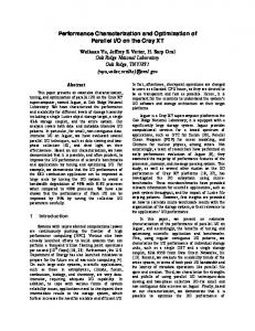
This normality assumption can be justified under the central-limit theorem since the Hotelling test statistic is a linear combination of the components of the data vector and, for the SKE task we are considering, these components are statistically independent random variables. B. Required Quantities of the Optical Coherence Imaging System The basic OCI system is quite simple in construction; an example is the free-space OCI system shown in Fig. 1. Generally, the measured output of an OCI system is directly related to the detected photocurrent. Therefore we will let this detected photocurrent be our OCI system output I共t兲. To compute the detectability as given in (1), we must first derive the photocurrent I共t兲 along with its mean 具具I共t兲典典 and its autocovariance function K共t , t⬘兲. Both the mean photocurrent data and the autocovariance function of the photocurrent data are derived for the case of unpolarized light, isotropic propagation through the system, and only normal incidence of the light propagating through the system. The mean photocurrent and autocovariance function can be extended past this simple case so that polarization and nonnormal incidence may be taken into account; however, within the scope of this paper the simple case will be considered to establish a benchmark performance. Our strategy in what follows is to show how we may express the mean and the autocovariance functions of the photocurrent data, and we will discover in the process that certain statistical moments of the source are needed. We will express these moments, in terms of the spectral characteristics of the source, as they arise. The photocurrent from the detector can be expressed simply as the number of photoelectrons N共t兲 created as a function of time by the incident electric field as

Fig. 1.

Basic free-space OCI system setup.

e I共t兲 =

⌬t

冕

t

N共t⬘兲dt⬘ ,

共7兲

t−⌬t

where e is the charge of an electron 共1.6⫻ 10−19 C兲 and ⌬t is the integration window associated with the detector. For the sake of simplicity, we can rewrite the photocurrent from Eq. (7) as e I共t兲 =

⌬t

冕

⬁

r共t − t⬘兲N共t⬘兲dt⬘ ,

再

where the function r共t兲 is defined as r共t兲 =

共8兲

−⬁

1 0 艋 t 艋 ⌬t 0 otherwise

冎

.

共9兲

The number of photoelectrons created is directly proportional to the electric field incident on the detector, which is proportional to the electric field emitted from the source. However, the electric field emitted from the broadband source and the creation of photoelectrons in the detection process have certain statistics associated with them. The broadband nature of the source ensures that the electric field emitted from the source will obey circular Gaussian statistics; also, it is well known that the creation of photoelectrons in the detection process obeys Poisson statistics.10 Hence N共t兲 may be referred to as a doubly stochastic Poisson random process.4,10 We will now look at the statistics of the source and the detection process and investigate how these noise components contribute to the mean photocurrent. Within the scope of this paper we will not consider any other noise components. 1. Mean Photocurrent To determine the mean photocurrent of the system, we must first look at the system input, the light source, and propagate this input through the system in order to determine the mean output. The light source emits an electric field Es共t兲 that we can decompose into a superposition of plane waves by taking its Fourier transform and expressing it as Es共t兲 =

冕

⬁

ˆ 共␻兲d␻ , exp共i␻t兲E s

共10兲

−⬁

where the caret denotes a function in the Fourier domain. The amplitude of these plane waves will be split at the beam splitter. One part of the field will propagate through the reference arm. Through this propagation it will experience a phase delay ␾1共␻ , t兲, which will account for the optical path length, dispersion, modulation, and other possible phase delays in the reference arm. This part of the field will also experience a loss of amplitude and possibly phase shifts upon reflection, which will be described by ␣ˆ 共␻兲; ␣ˆ 共␻兲 will account for absorption and nonequal reflection amplitudes within the reference arm as well as incorporate losses due to the beam splitter. Another part of the field will propagate through the specimen arm. Through this propagation it will experience a phase delay ␾2共␻ , t兲, which will account for the optical path length, dispersion, modulation, and other possible phase delays in the specimen arm. This part of the field will also experience a loss of amplitude and phase shifts from the speci-

Rolland et al.

Vol. 22, No. 6 / June 2005 / J. Opt. Soc. Am. A

men model, described mathematically by ␤ˆ 共␻兲; ␤ˆ 共␻兲 will account for absorption, nonequal reflection amplitudes, and phase shift upon reflection due to the specimen model as well as incorporate losses due to the beam splitter. These altered parts of the field will recombine at the beam splitter, and part of this sum of fields will propagate to the detector; the remaining part of the sum will propagate back toward the source. Therefore the total electric field at the detector may be related to the electric field at the source by E共t兲 =

冕

冕冕 ⬁

具具N共t兲典典 = ␳

−⬁

⫻

兵␣ˆ 共␻兲exp关i␾1共␻,t兲 + i␻t兴

ˆ 共␻兲d␻ . + ␤ˆ 共␻兲exp关i␾2共␻,t兲 + i␻t兴其E s

共11兲

For simplicity, hereafter we define

E共t兲 =

冕

⬁

ˆ 共␻兲d␻ . m共␻,t兲exp共i␻t兲E s

共13兲

−⬁

ˆ 共␻兲 are stochastic processes. In Eq. (13) both E共t兲 and E s Given that the source field Es共t兲 obeys circular Gaussian statistics, 具Es共t兲典 is zero. This implies that E共t兲 is also a Gaussian random process with 具E共t兲典 equal to zero. Taking the statistical average over all random processes, Eq. (8) may be rewritten to give the mean photocurrent as 具具I共t兲典典 =

具具 冕 冕 e

⌬t

e

=

⌬t

⬁

r共t − t⬘兲N共t⬘兲dt⬘

−⬁

G共␶兲 = 具E†s 共t − ␶兲Es共t兲典.

RA e␩0

G*共␶兲 = G共− ␶兲.

ˆ †共␻兲E ˆ 共␻⬘兲典 = 具E s s

e␩0

.

冕冕 ⬁

⬁

−⬁

−⬁

exp关i共␻⬘t2 − ␻t1兲兴

4␲2

冕冕 ⬁

⬁

−⬁

−⬁

exp关i共␻⬘t2 − ␻t1兲兴

⫻G共t2 − t1兲dt1dt2 共14兲

共15兲

1 =

In Eq. (17), 具具N共t兲典典 is the average of N共t兲 over the Poisson noise associated with detection and the Gaussian noise associated with the source field. On the other hand, ¯ 共t兲典 averages N ¯ 共t兲 over the Gaussian statistics only, 具N since the Poisson noise has already been averaged out to ¯ 共t兲. If we combine Eqs. (13) and (17), 具具N共t兲典典 can be get N rewritten as

exp i

−⬁

␻⬘ + ␻ 2

冊册

s G共s兲ds 共21兲

Inserting Eq. (21) into Eq. (18), we rewrite 具具N共t兲典典 as 具具N共t兲典典 = ␳

冕

⬁

兩m共␻,t兲兩2S共␻兲d␻ .

共22兲

−⬁

Finally, the mean photocurrent can be expressed as 具具I共t兲典典 =

共17兲

2␲

冕 冋冉 ⬁

␦共␻⬘ − ␻兲

= ␦共␻⬘ − ␻兲S共␻兲.

共16兲

From the conditional mean, the overall mean of the output is written as ¯ 共t兲典 = ␳具E†共t兲E共t兲典. 具具N共t兲典典 = 具N

4␲2

1 =

where R is the responsivity of the detector, A is the area of the detector, and ␩0 is the impedance of free space 共377 ⍀兲. The quantity ␳ is defined as

␳=

1

⫻ 具E†s 共t1兲Es共t2兲典dt1dt2

−⬁

RA

共20兲

ˆ 共␻兲 is This property ensures that the Fourier transform G ˆ real. Hereafter, G共␻兲 will be denoted S共␻兲 to represent the PSD of the source. ˆ †共␻兲E ˆ 共␻⬘兲典 from Eq. (18) may be exThe expectation 具E s s pressed by means of the inverse Fourier transform as

⬁

E†共t兲E共t兲 = ␳E†共t兲E共t兲,

共19兲

The stationarity assumption is related to the stability of the source. We may relax this assumption to quasistationarity in order to account for other sources of variation in the source field.4 The scalar autocovariance function has the property

Noting again that N共t兲 is a doubly stochastic Poisson random process, the conditional mean of N共t兲 is given by ¯ 共t兲 = N

共18兲

We will assume that the source field is a stationary random process and define the scalar autocovariance function of the source field as

典典

r共t − t⬘兲具具N共t⬘兲典典dt⬘ .

m*共␻,t兲m共␻⬘,t兲exp关i共␻⬘ − ␻兲t兴

−⬁

m共␻,t兲 = ␣ˆ 共␻兲exp关i␾1共␻,t兲兴 + ␤ˆ 共␻兲exp关i␾2共␻,t兲兴. 共12兲 Therefore Eq. (11) may be rewritten as

⬁

ˆ †共␻兲E ˆ 共␻⬘兲典d␻d␻⬘ . 具E s s

⬁

−⬁

1135

␳e ⌬t

冕

⬁

−⬁

r共t − t⬘兲

冋冕

⬁

−⬁

册

兩m共␻,t兲兩2S共␻兲d␻ dt⬘ . 共23兲

2. Autocovariance Function of the Photocurrent Now that we have an expression for the mean photocurrent, we next need the autocovariance function of the photocurrent in order to compute the detectability index. Starting with the autocovariance function expressed in Eq. (3) and substituting into it the expression in Eq. (8) for the various photocurrents, we can write the autocovariance function as

1136

J. Opt. Soc. Am. A / Vol. 22, No. 6 / June 2005

K共t,t⬘兲 =

冉 冊冕 冕 ⬁

2

e

⌬t

−⬁

Rolland et al.

⬁

r共t − t1兲r共t⬘ − t2兲KN共t1,t2兲dt1dt2 ,

lowing the same scheme as in Eq. (21), as

−⬁

ˆ †共␻⬘兲典 = ␦共␻⬘ − ␻兲G ˆ 共␻兲. ˆ 共␻兲E 具E s s

共24兲 where KN共t1 , t2兲 is the autocovariance function of the random process N共t兲. This autocovariance function is expressed as KN共t1,t2兲 = 具具N共t1兲N共t2兲典典 − 具具N共t1兲典典具具N共t2兲典典 = 具具N共t1兲典典␦共t1 − t2兲 + KN¯共t1,t2兲.

Combining Eqs. (28), (33), and (34) produces the condi¯ 共t1 , t2兲 as tional autocovariance function KN KN¯共t1,t2兲 = ␳2

−⬁

共26兲

The first term on the right-hand side of Eq. (26) can be expressed in terms of the statistical properties of the field as

†

†

−⬁

K共t,t⬘兲 =

冉 冊冕 冉 冊冕 冕 ⬁

2

e

r共t − t1兲r共t⬘ − t1兲具具N共t1兲典典dt1

⌬t

−⬁

2

⌬t

⬁

⬁

−⬁

−⬁

r共t − t1兲r共t⬘ − t2兲KN¯共t1,t2兲dt1dt2 共36兲

+ ␳2 tr关具E共t1兲E†共t2兲典具E共t2兲E†共t1兲典兴 ¯ 共t 兲典具N ¯ 共t 兲典 + ␳2 tr关具E共t 兲E†共t 兲典 = 具N 1 2 1 2 ⫻具E共t2兲E†共t1兲典兴,

共27兲

where tr is the three-dimensional trace function. Combining Eqs. (26) and (27), we can rewrite the conditional autocovariance function as KN¯共t1,t2兲 = ␳2 tr关具E共t1兲E†共t2兲典具E共t2兲E†共t1兲典兴

It is shown in Appendix A that if the PSD has as large a bandwidth as required by OCI, on the order of 1013 Hz, the second term on the right-hand side of Eq. (36) can be neglected so that the total autocovariance function can be approximated as

K共t,t⬘兲 ⬇

= ␳ tr关J共t1,t2兲J共t2,t1兲兴 = ␳ tr关J共t1,t2兲J 共t1,t2兲兴, 2

2

†

共28兲 where J共t1,t2兲 = 具E共t1兲E†共t2兲典.

共29兲

Now that we have the conditional autocovariance function in terms of the field at the detector, we can express it in terms of the field at the source. We define the autocovariance matrix of the source as G共␶兲 = 具Es共t兲E†s 共t − ␶兲典.

共30兲

This matrix has the following two properties: G†共␶兲 = G共− ␶兲, G共␶兲 = tr关G共␶兲兴.

冉 冊冕 e

⌬t

2

⬁

r共t − t1兲r共t⬘ − t1兲具具N共t1兲典典dt1 共37兲

−⬁

3. Specimen Model For the sake of our assessment, a specimen model, which is described mathematically by the term ␤ˆ 共␻兲, will be defined as a single layer bounded by two interfaces as shown in Fig. 2. The first interface is a boundary between air and the layer refractive index n. The second interface is a boundary between the layer refractive index n and a substrate refractive index n + ⌬n. A distance l separates the two interfaces. The expression for the reflection from this specimen model is given in Eq. (38), with the Fresnel reflections r1 and r2, and the phase delay ␦共␻兲 given by Eq. (39).

共31兲 共32兲

Next, J共t1 , t2兲 is computed as J共t1,t2兲 =

冕冕 ⬁

⬁

−⬁

−⬁

m共␻,t1兲m*共␻⬘,t2兲exp关i共␻t1 − ␻⬘t2兲兴

ˆ 共␻兲E ˆ †共␻⬘兲典d␻d␻⬘ . ⫻ 具E s s

共35兲

Hence the total autocovariance function is given by

+

= ␳ 具E 共t1兲E共t1兲典具E 共t2兲E共t2兲典 2

m共␻,t1兲m*共␻,t2兲m*共␻⬘,t1兲

ˆ 共␻兲G ˆ †共␻⬘兲兴d␻d␻⬘ . ⫻ tr关G

e

¯ 共t 兲N ¯ 共t 兲典 = ␳2具E†共t 兲E共t 兲E†共t 兲E共t 兲典 具N 1 2 1 1 2 2

⬁

⫻ m共␻⬘,t2兲exp关i共␻ − ␻⬘兲共t1 − t2兲兴

¯ 共t1 , t2兲 is the conditional autocovariance funcThe term KN tion, meaning that the Poisson statistics of the detection process are taken care of in the preceding term. This conditional autocovariance function is given by4

¯ 共t 兲N ¯ 共t 兲典 − 具N ¯ 共t 兲典具N ¯ 共t 兲典. KN¯共t1,t2兲 = 具N 1 2 1 2

冕冕 ⬁

共25兲

共34兲

共33兲

ˆ 共␻兲E ˆ †共␻⬘兲典 from Eq. (33) may be exThe expectation 具E s s pressed by means of the inverse Fourier transform, fol-

Fig. 2.

Illustration of the specimen model.

Rolland et al.

Vol. 22, No. 6 / June 2005 / J. Opt. Soc. Am. A

␤ˆ 共␻兲 = r1 + 共1 − r12兲r2␦2共␻兲, − ⌬n

1−n r1 =

1+n

,

r2 =

2n + ⌬n

,

共38兲

冉 冊

␦共␻兲 = exp i␻

nl c

.

共39兲

We have ignored multiple reflections because of the low reflected power at each interface for the changes in refractive index that we will consider. C. Task Definitions We shall investigate two tasks for assessing the performance of the system: a detection task and a resolution task. For the detection task, we will assess the smallest change in index of refraction at the second interface that the system can discriminate. Therefore we define the negative hypothesis H0 as no second interface, i.e., ⌬n = 0. The positive hypothesis H1 is defined as having a second interface, i.e., ⌬n = ⌬n0 ⫽ 0. For H1, ⌬n0 will be increased so that we can see how the detectability index and the AUC vary. To be sure that reflected fields from the two interfaces of the specimen model do not interfere for this task, we set the separation distance l to be the longest coherence length of the three theoretical sources considered. For the resolution task, we assess the smallest separation of the two interfaces of the layer that the system can discriminate. Therefore we have ⌬n equal to a constant. The negative hypothesis H0 for this task is defined as the two interfaces at the same location, i.e., l = 0. The positive hypothesis H1 corresponds to the two interfaces separated by a distance, i.e., l = l0 ⫽ 0. For H1, l0 will be increased so that we can see how the detectability index and the AUC vary for various values of the constant ⌬n for each theoretical source considered.

3. SIMULATION To properly simulate the detectability index associated with the detection task and the resolution task defined in Section 2, we must first define the theoretical setup and choose reasonable input parameters. We will consider the theoretical system to be the free-space interferometer system shown in Fig. 1. The scanning mechanism will be a mirror translating at a speed vm. As previously stated, we will investigate the detection task and the resolution task for three theoretical Gaussian PSDs. These normalized Gaussian PSDs are defined mathematically as11 S共␻兲 =

2共ln 2兲1/2

␲1/2⌬␻

再冋

exp − 2共ln 2兲1/2

␻ − ␻0 ⌬␻

册冎 2

,

共40兲

where ␻0 is the center angular frequency and ⌬␻ is the angular-frequency bandwidth (i.e., the spectral width) at FWHM. The angular-frequency bandwidth is related to the coherence length lc of the source as ⌬␻ =

8 ln 2 lc

c.

共41兲

The resolution may be considered to be half the coherence length.11 To define the three Gaussian PSDs, we consider

1137

coherence lengths of 2, 20, and 40 ␮m, corresponding to resolutions of 1, 10, and 20 ␮m and angular-frequency bandwidths of 8.32⫻ 1014 rad/ s, 8.32⫻ 1013 rad/ s, and 4.16⫻ 1013 rad/ s. Also, we consider the center angular frequency of all of these PSDs to be 1.98⫻ 1015 rad/ s, which corresponds to a wavelength of 950 nm. To establish the sampling frequency of the power spectrum of the source, we define the bandwidth B to be ⌬␻ / 2␲ expressed in hertz. The autocorrelation function that is the Fourier transform of the PSD is considered to be defined in a time range L of 3.5/ B. We define the extent of the Gaussian to be 3.5 times its sigma, given that below this value the Gaussian is very close to zero. The maximum optical frequency F of the PSD is given by 共␻0 + 1.75⌬␻兲 / 2␲. According to the Nyquist sampling condition, the sampling step ⌬T in the time domain should be at least 1 / 共2F兲. The number of samples in the PSD or its Fourier transform is then given by L / ⌬T. We computed that for the three values of the three coherence lengths in increasing order (i.e., 2, 20, and 40 ␮m) and the associated PSD, the minimum number of samples that the computation yields is 29, 179, and 346, respectively. In the simulations, each of the PSDs was sampled with 600 points over the angular frequency range of ␻0 − 1.75⌬␻ to ␻0 + 1.75⌬␻, which is well above the minimum required; this range minimizes sampling in the tails of each Gaussian PSD, where the PSDs have values near zero. Also, the power for each of these three theoretical sources is set to 3 mW. For ease in comparing the results, in the simulation we will vary no parameters other than the coherence length and therefore the angular-frequency bandwidth and the parameter to be varied for each task. We must also provide quantitative parameters for the values of ␣ˆ 共␻兲, ␾1共␻ , t兲, and ␾2共␻ , t兲 given in Eq. (12), the value of ⌬t given in Eq. (7), the values of R and A given in Eq. (16), and the value of n given in Eq. (39). The losses and phase shifts of the beam splitter are ignored, and the mirror is assumed to have a unit reflection for all frequencies: ␣ˆ 共␻兲 is 1. The phase terms ␾1共␻ , t兲 and ␾2共␻ , t兲 are set to ␻共2lr / c兲 + vmt and ␻共2ls / c兲, respectively. The constants lr and ls are the distances from the point where the field is split to the initial location of the reference mirror and the specimen, respectively. For the purpose of the simulation, ls is chosen to be 3 mm, and lr is chosen to be 3 mm less 28 ␮m. The speed of the mirror vm is chosen to be 0.154 m / s, and t is increased from zero by steps of 0.4 ␮s over the total scan time of 0.8 ms for a total of 2000 time samples. The detector integration time ⌬t is 4 ␮s (i.e., bandwidth is 125 KHz); thus time sampling at 2.5 MHz (i.e., every 0.4 ␮s) ensures that the Nyquist sampling condition will be satisfied. The responsivity R of the detector is assumed to be 1 for all frequencies, and the area A of the detector is chosen to be 0.79 mm2; these quantities result in a ␳ value of 1.3097⫻ 1010 m2 / 共V2s兲. The value of the refractive index n is set to 1.4. Finally, finite-width integrations, and more particularly trapezoidal numerical integrations, were performed in the simulations. A. Detection Task As previously stated for the detection task, we will assess the smallest change in refractive index at the second in-

1138

J. Opt. Soc. Am. A / Vol. 22, No. 6 / June 2005

terface that our system can discriminate. To be sure that the interference between the two interfaces of the specimen model does not influence this measure, we set the distance between the two interfaces l to 40 ␮m, the longest coherence length considered. The value of ⌬n0 is then increased from 0 to 3 ⫻ 10−5. The plots for the detectability index and the AUC versus the value of ⌬n0 for each coherence length considered are given in Fig. 3. B. Resolution Task For the task of resolution, we assess the smallest separation of the two interfaces of the layer defined in Section 2 that the system can discriminate. To compute the detectability index and the AUC for the resolution task, we chose a change in refractive index corresponding to (a) a 75% probability of detection 共AUC= 0.75兲, (b) the smallest change in refractive index corresponding to 100% probability of detection (AUC first reaches 1), and (c) twice the smallest change in refractive index corresponding to 100% probability of detection for the detection task for each of the three coherence lengths; these three refractive indices will be denoted ⌬n1, ⌬n2, and ⌬n3, respectively. These changes in refractive indices are ⌬n1 = 6.51⫻ 10−6, ⌬n2 = 3 ⫻ 10−5, and ⌬n3 = 6 ⫻ 10−5 for a coherence length of 2 ␮m; ⌬n1 = 2.06⫻ 10−6, ⌬n2 = 1.05⫻ 10−5, and ⌬n3 = 2.1

Fig. 3. Detection task. (a) Detectability index, (b) AUC for Gaussian sources of 2, 20, and 40 ␮m coherence length.

Rolland et al.

⫻ 10−5 for a coherence length of 20 ␮m; and ⌬n1 = 1.45 ⫻ 10−6, ⌬n2 = 9 ⫻ 10−6, and ⌬n3 = 1.8⫻ 10−5 for a coherence length of 40 ␮m. For each of the three coherence lengths, the value of l0 is increased from 0 to the coherence length so we can see how the detectability index and the AUC change with the separation distance l0. The plots for the detectability index and the AUC versus the value of l0, the separation distance, for each of the cases are given in Fig. 4.

4. DISCUSSION In this section we discuss the results of the simulation for both the detection task and the resolution task. Also, we reiterate the assumptions made in this paper and present the possible extensions of the mathematical framework provided. A. Detection Task As expected and as seen in Fig. 3, the increase in the detectability index and the AUC as a function of increasing change in refractive index signifies that it becomes easier for the observer to discriminate between a second interface and no second interface as the change in refractive index increases. Specifically, according to the plot of the AUC in Fig. 3(b), with the parameters used and the system modeled the observer can detect a second interface with 100% probability when a change in index of 3 ⫻ 10−5 occurs for a coherence length of 2 ␮m, 100% probability when a change in index of 1.05⫻ 10−5 occurs for a coherence length of 20 ␮m, and 100% probability when a change in index of 9 ⫻ 10−6 occurs for a coherence length of 40 ␮m. These three changes in refractive index constitute the benchmark performance for the detection task. Overall, a longer coherence length source has a greater detectability index for a lower change in refractive index. This phenomenon stems from the fact that under exactly the same conditions, a longer coherence length source has larger values for the X vector than a shorter coherence length source, as shown in Fig. 5. B. Resolution Task As expected and as seen in Figs. 4(d)–4(f), the AUCs increase as the separation distance between the two interfaces increases. However, within a separation distance that is less than half the coherence length of the source, oscillations are observed in both the detectability index [Figs. 4(a)–4(c)] and the AUCs [Figs. 4(d)–4(f)], at least for the smallest change in refractive index indicated in the curve definitions; these oscillations correspond to interference from fields reflected from the first and second interfaces of the specimen model. Indeed, when the separation of the two interfaces of the specimen model is smaller than half the coherence length of the source, the reflected fields from the two interfaces interfere constructively if the optical path difference between the two layers is a multiple of the central wavelength of the source. Similarly, for separations corresponding to out-of-phase interfering fields, the fields interfere destructively. As the separation increases, the contrast of the fringes decreases as a consequence of the nonmonochromatic light field. Upon first observing these oscillations, we validated that

Rolland et al.

Vol. 22, No. 6 / June 2005 / J. Opt. Soc. Am. A

1139

Fig. 4. Resolution task. Detectability index versus separation distance for sources with coherence length of (a) 2 ␮m, (b) 20 ␮m, and (c) 40 ␮m. AUC versus separation distance for sources with coherence length of (d) 2 ␮m, (e) 20 ␮m, and (f) 40 ␮m.

1140

J. Opt. Soc. Am. A / Vol. 22, No. 6 / June 2005

Rolland et al.

in the detection task study; the shorter the coherence length, the higher the probability of distinguishing between two separated layers or two coinciding layers for refractive indices below the detection limit determined by the detection task. Thus the resolution performance of the system depends on both the broadband source and the specimen being imaged. For the change in refractive index ⌬n3, while the detectability index has the same general behavior as the change in refractive indices ⌬n1 and ⌬n2, it can be seen that the AUC has changed tremendously. In fact, the AUC shows that for any separation distance greater than zero, the observer can discriminate between two separated layers and two coinciding layers with 100% probability. This finding is in agreement with the following statement by Harris12: “In the classic case of resolving two point sources in the presence of Gaussian noise, results indicate that although diffraction increases the difficulty of rendering a correct binary decision, it does not prevent a correct binary decision from being made, no matter how closely spaced the two point sources may be” (p. 611).

Fig. 5. Signal X for the detection task given ⌬n0 = 0.1 for coherence length sources of (a) 40 ␮m and (b) 2 ␮m.

the oscillations’ period corresponded to optical separations that are multiples of the source’s central wavelength. Although this phenomenon is not speckle, since we are dealing only with two layers rather than with a scattering medium, it is reminiscent of speckle, which corresponds to multiple-scatterers’ interference for interferences localized within the coherence length of the source. In practice, given a specimen with varying properties such as unequal thickness layers or slight inhomogeneities in the refractive index defining a layer, the rapid oscillations will be averaged out. Such averaging may also apply when new sources of system noise are considered. Thus we expect that in practice, these high-frequency oscillations will have no effect on system optimization. Interestingly, even when the layer separation is beyond half the coherence length of the source, the observer can discriminate between two separated layers and two coinciding layers with only ⬍100% probability for the smallest change in index of refraction. Also, through inspection of the AUC in Figs. 4(d)–4(f), it can be seen that for shorter coherence lengths, the resolution performance of the system depends less on the detection limit established

Although this statement concerns incoherent imaging, it is easily extended to the case of two layers in OCI. Therefore for a sufficient change in refractive index at the second interface, there is a 100% probability of distinguishing between two separated layers and two coinciding layers. This sufficient change in refractive index is approximately ⌬n3. Thus for each of the three theoretical sources, the resolution benchmark is 100% probability of discrimination of two separated layers from two coinciding layers for ⌬n 艌 ⌬n3 for the corresponding source regardless of l0. This finding is further supported by previous observation by Richards-Kortum and associates, who state that “changes in scattering occur on a microscopic spatial scale well below the typical resolution of OCT imaging systems, yet these changes still impact OCT images” (Ref. 13, p. 465). C. Assumptions and Possibilities Although the mathematics for the mean and autocovariance of the photocurrent output of the OCI system were derived for the simple case of unpolarized light, an isotropic specimen model, and normal incidence of the propagating beam, these derivations can be extended to include polarization dependence, a nonisotropic specimen, and nonnormal incidence. We will include these cases as part of future work. The three PSDs considered within this paper are all the commonly used Gaussian shapes. However, the mathematical framework provided allows for any arbitrary PSD to be used. We have done precisely this in a previously published study.14 Furthermore, the demonstrated system did not include any noise other than the Gaussian noise from the source and the Poisson noise of the detection process; this system was simulated in order to verify that the model behaves as expected. This model provides the basic framework for which inclusion of more-realistic system components and other sources of noise can be carried out for any general

Rolland et al.

Vol. 22, No. 6 / June 2005 / J. Opt. Soc. Am. A

OCI system. Also, the benchmark performance introduced is set forth so that in the future, the results obtained with more-complex models can be compared with the results of the simple OCI system modeled in the current study.

5. CONCLUSION

APPENDIX A By performing order-of-magnitude estimation, we will show that the Poisson statistics’ contribution to the autocovariance dominates the Gaussian statistics’ contribution to the autocovariance. The Gaussian statistics’ contribution to the autocovariance of the photocurrent can be written as

冉 冊冕 冕 e

2

⌬t

⬁

⬁

−⬁

−⬁

r共t − t1兲r共t⬘ − t2兲KN¯共t1,t2兲dt1dt2 , 共A1兲

where

冕冕 ⬁

KN¯共t1,t2兲 = ␳2

−⬁

m共␻,t兲 = ␣ˆ 共␻兲exp关i␾1共␻,t兲兴 + ␤ˆ 共␻兲exp关i␾2共␻,t兲兴 = C1共␻,t兲 + C2共␻,t兲.

共A3兲

ˆ †共␻⬘兲c can be expanded as ˆ 共␻兲G The term trbG ˆ †共␻⬘兲c = G ˆ 共␻兲G ˆ * 共 ␻ ⬘兲 + G ˆ 共␻兲G ˆ * 共 ␻ ⬘兲 ˆ 共␻兲G trbG xx xy xx yx

We have presented the basics of a model to optimize and assess the performance of a general OCI system based on the basis of task performance and statistical decision theory. This general model was adapted to a simple OCI system to allow us to assess the performance of the system in terms of a specific detection task and a specific resolution task. For a task-based performance assessment on the detection task for the simple OCI system presented, the smallest change in refractive index detectable was shown to be dependent on the angular-frequency bandwidth of the source. Considering the system parameters, a benchmark performance for the detection task is that a change in refractive index of 3 ⫻ 10−5 is detectable for a Gaussian source of 2 ␮m coherence length, a change in refractive index of 1.05⫻ 10−5 is detectable for a Gaussian source of 20 ␮m coherence length, and a change in refractive index of 9 ⫻ 10−6 is detectable for a Gaussian source of 40 ␮m coherence length, with 100% probability. Furthermore, the performance of this system based on the resolution task was shown to be dependent on the specimen model and the angular-frequency bandwidth of the source for small changes in the refractive index at the second interface. Also, the performance of the system based on the resolution task for changes in refractive index well beyond the detection limit was seen to agree with previous findings. This agreement is that for infinitely close interfaces of sufficient change in index, i.e., changes well beyond the detection limit of 100%, the binary classification task of whether there are two separated layers or two coinciding layers can be carried out with 100% accuracy.

KG共t,t⬘兲 =

1141

⬁

m共␻,t1兲m*共␻,t2兲m*共␻⬘,t1兲m共␻⬘,t2兲

−⬁

ˆ 共␻兲G ˆ †共␻⬘兲兴d␻d␻⬘ . ⫻ exp关i共␻ − ␻⬘兲共t1 − t2兲兴tr关G 共A2兲 The term m共␻ , t兲 is defined as

ˆ 共␻兲G ˆ * 共 ␻ ⬘兲 + G ˆ 共␻兲G ˆ * 共 ␻ ⬘兲 +G yx yy xy yy 2

=

2

兺 兺 Gˆ

ˆ* mn共␻兲Gmn共␻⬘兲,

x = 1,

y = 2.

m=1 n=1

共A4兲 Using the definition in Eq. (A3) and the expansion in Eq. (A4), Eq. (A2) can be rewritten as 2

KN¯共t1,t2兲 = ␳2

2

2

2

2

2

兺兺兺兺 兺 兺

h=1 j=1 k=1 l=1 m=1 n=1

冕

⬁

Ch共␻,t1兲Cj*共␻,t2兲

−⬁

ˆ 共␻兲d␻ ⫻ exp关i␻共t1 − t2兲兴G mn ⫻

冕

⬁

Ck* 共␻⬘,t1兲C1共␻⬘,t2兲exp关− i␻⬘共t1 − t2兲兴

−⬁

ˆ * 共␻⬘兲d␻⬘ . ⫻G mn

共A5兲

Equation (A5) has a total of 64 terms. The two integration terms are Fourier transforms of the composite functions ˆ 共␻兲 and C* 共␻⬘ , t 兲C 共␻⬘ , t 兲G ˆ * 共␻⬘兲; Ch共␻ , t1兲Cj*共␻ , t2兲G mn 1 l 2 k mn we are concerned with the behavior of these autocovariance terms only in terms of the difference between t1 and t2. If we assume that the functions ␣ˆ 共␻兲 and ␤ˆ 共␻兲 have very broad spectral responses, i.e., the spectral responses of these functions are much greater than the bandwidth ˆ 共␻兲, and that the phase of the PSDs represented by G mn functions ␾1共␻ , t兲 and ␾2共␻ , t兲 are real, these Fourier transform terms will have widths in the time 共t1 − t2兲 domain on the order of the inverse of the frequency bandwidth of the PSDs. Also, by the central ordinate theorem, these terms will have a peak value proportional to the integral of the PSDs. We will not concern ourselves with the integrations in time in Eq. (A1). These integrations will serve only to smooth the autocovariance. If we use angular-frequency bandwidths of the PSDs on the order of 2␲ ⫻ 1013 rad/ s, the Fourier transform has a width in the time domain on the order of 1 ⫻ 10−13 s. Assuming a normalized area of 1 for the PSDs for ease and using the value of 1 ⫻ 1010 m2 / 共V2s兲 for ␳, we can consider the autocovariance as an equivalent delta function with KN¯共t1,t2兲 = O关6.4 ⫻ 10−5␦共t1 − t2兲兴,

共A6兲

where O represents “on the order of.” The autocovariance term of the Poisson statistics 具N共t1兲典␦共t1 − t2兲, with the same broad approximations, is equivalently 具具N共t1兲典典␦共t1 − t2兲 = O关1 ⫻ 1010␦共t1 − t2兲兴.

共A7兲

Thus the Gaussian statistics’ contribution to the autocovariance can be considered negligible in comparison with that of the Poisson statistics.

1142

J. Opt. Soc. Am. A / Vol. 22, No. 6 / June 2005

Rolland et al.

ACKNOWLEDGMENTS We thank Harry Barrett and Kyle Myers for stimulating discussion about this work. This work was supported in part by National Cancer Institute Contract CA87017, National Science Foundation Division of Information and Intelligent Systems grant 00-82016, the Division of Information Technology Research, the U.S. Army Research Office, the University of Central Florida Presidential Instrumentation Initiative, the Defense Advanced Research Projects Agency, the National Science Foundation Procurement Technical Assistance Program, and the Florida Photonics Center of Excellence.

5.

Corresponding author Jannick Rolland’s e-mail address is [email protected].

9.

6. 7. 8.

10. 11.

REFERENCES 1.

2. 3. 4.

D. Huang, E. A. Swanson, C. P. Lin, J. S. Schuman, W. G. Stinson, W. Chang, M. R. Hee, T. Flotte, K. Gregory, C. A. Puliafito, and J. G. Fujimoto, “Optical coherence tomography,” Science 254(5035), 1178–1181 (1991). A. F. Fercher, W. Drexler, C. K. Hitzenberger, and T. Lasser, “Optical coherence tomography—principles and applications,” Rep. Prog. Phys. 66, 239–303 (2003). J. M. Schmitt, “Optical coherence tomography (OCT): a review,” IEEE J. Sel. Top. Quantum Electron. 5, 1205–1215 (1999). H. H. Barrett and K. J. Myers, “Image quality,” in Foundations of Image Science, Series in Pure and Applied

12. 13. 14.

Optics (Wiley, Hoboken, New Jersey, 2004), Chap. 14, pp. 913-1000. M. A. Kupinski, J. W. Hoppin, E. Clarkson, and H. H. Barrett, “Ideal-observer computation in medical imaging with use of Markov-chain Monte Carlo techniques,” J. Opt. Soc. Am. A 20, 430–438 (2003). E. Clarkson and H. H. Barrett, “Approximation to idealobserver performance on signal-detection tasks,” Appl. Opt. 39, 1783–1793 (2000). W. E. Smith and H. H. Barrett, “Hotelling trace criterion as a figure of merit for the optimization of imaging systems,” J. Opt. Soc. Am. A 3, 717–725 (1986). P. Bonetto, J. Qi, and R. M. Leahy, “Covariance approximation for fast and accurate computation of channelized Hotelling observer statistics,” IEEE Trans. Nucl. Sci. 47, 1567–1572 (2000). H. Hotelling, “The generalization of Student’s ratio,” Ann. Math. Stat. 2, 360–378 (1931). J. W. Goodman, Statistical Optics (Wiley, New York, 2000). C. Akcay, P. Parrein, and J. P. Rolland, “Estimation of longitudinal resolution in optical coherence imaging,” Appl. Opt. 41, 5256–5262 (2002). J. L. Harris, “Resolving power and decision theory,” J. Opt. Soc. Am. 54, 606–611 (1964). B. E. Bouma and G. J. Tearney, eds., Handbook of Optical Coherence Tomography (Marcel Dekker, New York, 2002). J. P. Rolland, J. O’Daniel, E. Clarkson, K. Cheong, C. A. Akcay, P. Parrein, T. DeLemos, and K. S. Lee, “AUC-based resolution quantification in optical coherence tomography,” in Medical Imaging: Image Perception, Observer Performance and Technology Assessment, D. P. Chakraborty and M. P. Eckstein, eds., Proc. SPIE 5372, 334–353 (2004).