The AVINOR Aeroelastic Simulation Code and Its ... - CiteSeerX

50th AIAA/ASME/ASCE/AHS/ASC Structures, Structural Dynamics, and Materials Conference
17th 4 - 7 May 2009, Palm Springs, California

AIAA 2009-2601

The AVINOR Aeroelastic Simulation Code and its Application to Reduced Vibration Composite Rotor Blade Design Bryan Glaz∗, Peretz P. Friedmann†, Li Liu‡, Devesh Kumar§ and Carlos E. S. Cesnik¶ Department of Aerospace Engineering, The University of Michigan, Ann Arbor, MI, 48109, USA

The Active Vibration and Noise Reduction (AVINOR) aeroelastic simulation code for helicopter rotor blades is described. AVINOR is a research code that has been developed at UCLA and the University of Michigan for the purpose of conducting computationally efficient aeroelastic response analyses while maintaining a level of fidelity so as to be suitable for preliminary design of helicopter rotor blades. The current capabilities of AVINOR are illustrated by considering aeroelastic tailoring of a composite rotor blade for minimum vibration over the entire flight envelope. The AVINOR composite blade model is based on geometrically nonlinear kinematics suitable for moderate deflection analysis and the University of Michigan/Variational Asymptotic Beam Sectional (UM/VABS) analysis is used for cross-sectional modeling. A surrogate-based optimization (SBO) approach is utilized to locate a blade design which exhibits the best trade-off between reducing vibration due to blade-vortex interaction (BVI) at low advance ratios, and alleviating vibration due to dynamic stall which occurs at high advance ratios.

Nomenclature bi Bi c CW Cd0 Cdf D F4X , F4Y , F4Z

Undeformed coordinate system Deformed coordinate system (see Fig. 3) Blade chord Helicopter weight coefficient Blade profile drag coefficient Flat plate drag coefficient Vector of design variables

g(D) H, A, B, C, D JACF JP , J V ki m0 M4X , M4Y , M4Z

Constraints

Nb

Number of rotor blades

4/rev hub shears, non-dimensionalized by m0 Ω2 R2

Composite cross-sectional parameters Active control objective function Rotor power and vibration passive optimization objective functions Initial twist as a function of x1 Baseline mass per unit length 4/rev hub moments, non-dimensionalized by m0 Ω2 R3

∗ Postdoctoral

Researcher, Member AIAA. Bagnoud Professor, Fellow AIAA, AHS ‡ Postdoctoral Researcher, Member AIAA. § Ph.D. Candidate ¶ Professor, Associate Fellow AIAA † Fran¸ cois-Xavier

1 of 34 Copyright © 2009 by B. Glaz, P. P. Friedmann, L. Liu, D. Kumar, and C. E. S. Cesnik. Published by the American Institute of Aeronautics and Astronautics, Inc., with permission.

Nc Ndv q Q R s Sij Ti wi Wu Wα Vj (x1 ) XF A , ZF A

y

Number of behavior constraints Number of design variables Finite element degrees of freedom Weighting matrix on objectives to be reduced Blade radius Predicted error in surrogate objective function 2-D warping finite element shape functions Deformed coordinate system (see Fig. 3) 3-D warping displacements Weighting matrix on control input Active control weight setting 1-D warping nodal values Longitudinal and vertical offsets between rotor hub and helicopter aerodynamic center, see Fig. 11 Longitudinal and vertical offsets between rotor hub and helicopter center of gravity, see Fig. 11 Generalized modal coordinates

Symbols αd βp δf γ11 , γ12 , γ13

Flight descent angle, see Fig. 11 Blade precone angle Flap deflection angle 1-D axial and shear strain measures

XF C , ZF C

Γ11 , Γ12 , Γ13 , Γ22 , Γ23 , Γ33

3-D Strain components

Γj2 κi κ ¯i λk ζk , ω k µ Π (x2 , x3 ) ψ Ω ωF 1 , ωL1 , ωT 1 ωL , ω U σ σ11 , σ12 , σ13 , σ22 , σ23 , σ33

States associated with dynamic stall model Moment strains in the Bi coordinate system Moment strains in the Ti coordinate system Hover stability eigenvalue for k th mode Real and imaginary parts of λk respectively Advance ratio Stress/strain influence coefficients Azimuth angle Rotor angular speed Fundamental rotating flap, lead-lag and torsional frequencies, /rev Lower and upper bounds for frequency constraints, /rev Rotor solidity

θpt

Built-in pretwist angle

3-D Stress components

I.

Introduction

P

recise modeling of a helicopter rotor blade’s aeroelastic response is critical for accurate vibration and acoustic predictions, and is an inherently multidisciplinary problem characterized by the interaction of the complex rotary wing aerodynamic environment with nonlinear structural dynamics. Rotary wing aerodynamic models must account for unsteadiness, non-uniform inflow distribution, a reverse flow region, and possibly dynamic stall effects. In addition, the structural dynamic model must account for geometric nonlinearities as well as non-classical effects associated with composite beams such as transverse shear deformation, cross-sectional warping, and elastic coupling due to material anisotropy. Due to the level of complexity, comprehensive simulation codes are required to combine these models within an aeroelastic stability and response solution framework. Relatively efficient analysis codes that retain a suitable level of fidelity can be used for preliminary design studies. For example, such codes combined with structural optimization techniques have generated reduced vibration designs which have been experimentally validated.1–3 Although the analysis 2 of 34 American Institute of Aeronautics and Astronautics

Rotor Hub

Pitch Link

Swashplate

(a) Dual servo flap configuration

(b) Single plain flap configuration

Figure 1. Helicopter rotor blades with partial span trailing edge flaps

codes employed in Refs. 1 – 3 did not always accurately predict the experimentally measured loads, the optimum designs corresponded to reduced vibrations in wind tunnels. The AVINOR (Active Vibration and Noise Reduction) analysis code has been developed over the years at UCLA and the University of Michigan to balance the need for computational efficiency so that it can be used for research purposes, while retaining a suitable level of fidelity so as to be suitable for preliminary design studies. The simulation code has been used primarily to investigate active and passive approaches to improved rotor blade design. For active control, partial span actively controlled flaps (ACF’s), which are depicted in Fig. 1, can be modeled. Partial span ACF’s have emerged as an attractive means of active control due their low power requirement compared to blade root actuation approaches.4, 5 The optimal deflections for various combinations of vibration reduction, noise reduction, and performance enhancement are determined by a variant of the higher-harmonic control algorithm.6–10 In addition to only utilizing active control, AVINOR has also been used to develop a combined active/passive multi-objective design methodology based on efficient optimization methods classified as surrogate-based optimization (SBO).11–14 The AVINOR aerodynamic model consists of four components - (1) an attached flow 2-D time domain unsteady aerodynamic model that accounts for compressibility and time-varying freestream Mach numbers,15 (2) a semi-empirical dynamic stall model used for the portions of the blade in the separated flow regime,16, 17 (3) a free-wake model which calculates the non-uniform inflow distribution at closely spaced azimuthal steps,18–21 and a (4) reverse flow model. The unsteady aerodynamic loads and pressure distribution are required for vibratory load, acoustic, and performance calculations. The structural dynamic model is based on the finite element method which is used to discretize 1-D beam equations that account for moderately large deflections.22, 23 Recently, the structural dynamic model described in Refs. 22 and 23 was upgraded by using the 2-D finite element code UM/VABS ( University of Michigan/ Variational Asymptotic Beam Sectional Analysis)24–26 as the composite beam cross-sectional analysis. The UM/VABS26 sectional analysis represents the state-of-the-art in computationally efficient modeling of composite blades. By using UM/VABS as the cross-sectional analysis, the upgraded AVINOR structural dynamic model27 can more accurately calculate stress/strain distributions compared to the original model described in Refs. 22 and 23. Furthermore, the improved composite blade model is not susceptible to large errors in the predicted torsional rigidity due to the uniaxial stress assumption.28 The objectives of this paper are to document the current capabilities of AVINOR, and to illustrate the usefulness of AVINOR combined with SBO for aeroelastic tailoring of composite rotor blades for vibration reduction over the entire flight envelope. The design of composite blade sections for improved passive23, 29–33 and active34 characteristics has been investigated in several computational studies. In addition, aeroelastic tailoring of composite blades has been experimentally shown to be a viable means of designing reduced vibration blades.35 In contrast to previous computational investigations of aeroelastic tailoring,23, 29–33 the study presented in this paper deals with obtaining the best design for simultaneous vibration reduction at low advance ratios where blade-vortex interaction (BVI) induces high vibration levels, and at high advance ratios where dynamic stall is the dominant source of vibration. The multi-objective problem of optimizing a blade for vibration reduction over the entire flight envelope was considered in Ref. 12. However, the study in Ref. 12 was limited to the design of a simplified model of an isotropic blade.

3 of 34 American Institute of Aeronautics and Astronautics

II.

Aeroelastic Response Model

The aeroelastic response analysis in AVINOR can represent the behavior of hingeless, bearingless, or articulated rotor blades with actively controlled flaps. The key ingredients of the simulation code are: (1) the structural dynamic model, (2) the unsteady aerodynamic model, and (3) a coupled trim/aeroelastic response solution required for the computation of the blade response and aeroelastic stability in hover. The governing aeroelastic equations of motion are formulated using a finite element discretization of Hamilton’s principle, and are of the form, ˙ ψ)]q˙ + [K(q, q, ˙ q ¨ , ψ)]q + F(q, q, ˙ q ¨ , ψ) = 0, [M(q, ψ)]¨ q + [C(q, q,

(1)

where M, C, K are the nonlinear finite element mass, damping, and stiffness matrices, F is the load vector, ˙ denotes a derivative with respect to time, i.e. ∂() . q is the vector of finite element degrees of freedom, and () ∂ψ A description of the various components of Eq. 1 are provided next. II.A.

Structural Dynamic Model

The structural dynamic model is based on an analysis described in Refs. 22 and 23 and is capable of modeling composite blades with transverse shear deformations, cross-sectional warping, and swept tips. The structural dynamic model was recently upgraded by using UM/VABS26 as the cross-sectional analysis. A detailed validation study on the combination of the original structural dynamic model with UM/VABS can be found in Ref. 27. The strain relations, constitutive relations, the resulting strain energy relations, and the kinetic energy relations required to model the blade are described in this section. II.A.1.

Strain Relations

Consider a beam idealized as a reference line, with a cross-section depicted in Fig. 2. A coordinate system parallel to the orthogonal unit vectors bi for i = 1, 2, 3 is fixed at each point along the undeformed reference line, where b1 is tangent to the reference line and b2 , b3 are orthogonal to b1 . The coordinates x2 , and x3 correspond to the b2 , b3 unit vectors, while x1 denotes the axial location of the cross-section. b3 und

efo

rm

ed

b2

ref

ere

nce

line

b1

Figure 2. Undeformed coordinate system.

From Ref. 22, the non-zero components of the strain tensor in the bi system associated with the original model from Yuan and Friedmann (YF) blade model, are given by: Γ11 = γ11 +w1,1 + k1 x3 w1,2 − x2 w1,3 − x2 κ ¯ 3 − 2γ12,1 + 2k1 γ13 1 2 2 − x3 −¯ κ2 − 2γ13,1 − 2k1 γ12 + x2 + x23 κ ¯1 (2) 2 2Γ12 = 2γ12 + w1,2 − x3 κ ¯1

(3)

2Γ13 = 2γ13 + w1,3 + x2 κ ¯1 ,

(4)

where ( ),i denotes a derivative with respect to the xi coordinate. In Eqs. 2 – 4, the 1-D axial and shear strain measures at the reference line, which are functions of the x1 coordinate only, are given by γ11 , γ12 , and γ13 respectively. The initial twist is denoted by k1 . The out-of-plane warping displacements w1 are 4 of 34 American Institute of Aeronautics and Astronautics

functions of x1 , x2 , and x3 . Note that the original YF formulation does not include in-plane warping nor in-plane strains. The 1-D “moment strains”,25 κ ¯ i , are with respect to a coordinate system parallel to the Ti basis vectors shown in Fig. 3 and represent the differences between the deformed and initial states of the twist and bending curvatures. The elastic twist is given by κ ¯ 1 , while κ ¯ 2 and κ ¯ 3 are the moment strains corresponding to bending. Since the helicopter rotor blade is assumed to have no initial curvature in the YF model, the bending moment strains are equal to the deformed bending curvatures. In the UM/VABS formulation, the moment strains are written with respect to the Bi coordinate system and denoted by κi . The Ti and Bi systems differ due to transverse shear deformation since T1 is tangent to the deformed reference line, while B1 is normal to the deformed cross-section. With the assumption of no initial bending curvature, the elastic B3

T3 2γ13

T1 nce

def

re efe dr

e

lin

B1

e

orm

deformed cross-section

Figure 3. Coordinate systems which differ due to transverse shear deformations.

twist and the deformed bending curvatures in the Ti system are transformed to the Bi coordinate system by:36 κ ¯ 1 = κ1 (5) κ ¯ 2 = κ2 − 2γ13,1 − 2k1 γ12

(6)

κ ¯ 3 = κ3 + 2γ12,1 − 2k1 γ13 .

(7)

The YF strain relations can be rewritten in a form which is consistent with the UM/VABS formulation by substituting Eqs. 5 – 7 into Eqs. 2 – 4. The strain relations corresponding to the combined YF and UM/VABS blade model, referred to as the YF/VABS model, are: 2 (8) Γ11 = γ11 + w1,1 + k1 x3 w1,2 − x2 w1,3 − x2 κ3 + x3 κ2 + 21 x22 + x23 κ1 2Γ12 = 2γ12 + w1,2 − x3 κ1 + f12 (w2 , w3 )

(9)

2Γ13 = 2γ13 + w1,3 + x2 κ1 + f13 (w2 , w3 )

(10)

Γ22 Γ23 Γ33

= f22 (w2 ) 6= 0, = f23 (w2 , w3 ) 6= 0, = f33 (w3 ) 6= 0,

(11)

where fij represent the contributions from the in-plane warping to the strain field. Note that by utilizing UM/VABS, the strain due to in-plane warping is accounted for. In UM/VABS, the warping displacements are discretized over the cross-section using the finite element approach. The UM/VABS warping displacements can be written as wi (x1 , x2 , x3 ) = Sij (x2 , x3 ) Vj (x1 ) , i = 1, 2, 3 and j = 1, 2, . . . , NV . 5 of 34 American Institute of Aeronautics and Astronautics

(12)

In Eq. 12, Sij are 2-D finite element shape functions, Vj are the 1-D nodal values of the warping displacement over the cross-section, and NV is the number of nodal degrees of freedom. II.A.2.

Constitutive relations

The constitutive relation for an anisotropic material is given by σ = DΓ Γ

(13)

T σ = [σ11 σ12 σ13 σ22 σ23 σ33 ]

(14)

where

T

Γ = [Γ11 2Γ12 2Γ13 Γ22 2Γ23 Γ33 ] ,

(15)

and DΓ is the 6 × 6 symmetric compliance matrix. Note that the original YF model employs the uniaxial stress assumption, i.e. σ22 = σ23 = σ33 = 0. Although the uniaxial stress assumption was considered valid for composite thin-walled structures in Ref. 22, it was demonstrated in Refs. 25 and 28 that this simplification may lead to significant errors in the torsional rigidity of a thin-walled composite boxbeam. Therefore, while the uniaxial stress simplification may lead to acceptable results for some composite cross-sections, the only way to ensure correct results for all cases is to employ a formulation, such as the one associated with UM/VABS, which does not neglect in-plane stresses. II.A.3.

Strain energy relations

The relation for strain energy, Us , is Z

L

ZZ

2Us = 0

ΓT σ dA dx1 ,

(16)

A

where L is the length of the beam, and A is the cross-sectional area of the structural member. After substitution of Eqs. 8 – 11 and Eq. 13 into Eq. 16, the strain energy will be a function of the following 1-D parameters: γ11 , 2γ12 , 2γ13 , κ1 , κ2 , κ3 and Vj , i.e. 2Us = f γ11 , 2γ12 , 2γ13 , κ1 , κ2 , κ3 , Vj . (17) However, in general there will be hundreds – thousands of nodes associated with the 2-D finite element discretization of the cross-section, and thus Eq. 17 will be a function of hundreds – thousands of nodal degrees of freedom Vj . Therefore, UM/VABS employs the variational asymptotic method25 in order to reduce the order of Eq. 17. The variational asymptotic approach produces an approximation of Us which is not a function of the 1-D warping variables Vj , i.e. ˜s = f˜ (γ , 2γ , 2γ , κ , κ , κ ) , 2Us ∼ = 2U 11 12 13 1 2 3

(18)

˜s and f˜ are the approximations of Us . The approximation of Us is obtained by minimizing the strain where U energy with respect to warping, which results in warping recovery relations for the nodal displacements Vj . The warping recovery relations are functions of the 1-D strain measures, γ11 , 2γ12 , 2γ13 , κ1 , κ2 , and κ3 . Expansion of Eq. 18 yields the YF/VABS strain energy, Z L ˜s = 2 2U (u1 + u2 ) dx1 (19) 0

where     1 u1 =  2   

γ11 2γ12 2γ13 κ1 κ2 κ3

T          

        

H11 H12 H13 H14 H15 H16

H12 H22 H23 H24 H25 H26

H13 H23 H33 H34 H35 H36

H14 H24 H34 H44 H45 H46

H15 H25 H35 H45 H55 H56

H16 H26 H36 H46 H56 H66


         

γ11 2γ12 2γ13 κ1 κ2 κ3

         

(20)

and

2

u2 = κ1 [(A22 + 2B12 ) γ11 + B22 κ1 + (2B23 + C22 ) κ2 + (2B24 + D22 ) κ3 ] .

(21)

The cross-sectional parameters, Hij , A22 + 2B12 , B22 , 2B23 + C22 , and 2B24 + D22 consist of integrals over the cross-section and are output by the VABS ‘Generalized Timoshenko model” with the “trapeze effect”.25 Note that while UM/VABS26 contains features which are unique among other VABS implementations, it does not output the higher order terms A22 + 2B12 , B22 , 2B23 + C22 , and 2B24 + D22 . In the YF/VABS model the trapeze effect is treated by setting A22 = H55 + H66 and all other elements of A, B, C, and D to zero as in Refs. 37 and. 38. The cross-sectional parameters output by UM/VABS are required as inputs to the YF beam equations. Note that the original YF strain energy contained terms that are not present in the VABS formulation described in Ref. 25. Furthermore, VABS outputs cross-sectional parameters which are not present in the original YF strain energy. However, the differences between the formulations are associated with higher order effects and thus do not prevent coupling between the two models. A detailed analysis of which cross-sectional parameters from the original YF formulation can be replaced with their VABS counterparts is provided in Ref. 27. II.A.4.

Kinetic energy relations

The kinetic energy cross-sectional properties calculated by UM/VABS are given in Eqs. 22 – 27, ZZ m≡ ρ dA

(22)

A

ZZ mx2 ≡

ρx2 dA

(23)

ρx3 dA

(24)

A

ZZ mx3 ≡

A

ZZ Im22 ≡

2

A

ρx3 dA

ZZ Im33 ≡

2

(25)

ρx2 dA

(26)

ρx2 x3 dA

(27)

A

ZZ Im23 ≡

A

where ρ is the material density. The YF model requires the same kinetic energy cross-sectional parameters given by Eqs. 22 – 27 as inputs. In addition, the YF model also requires cross-sectional properties associated with the kinetic energy due to warping velocities.22 Since warping velocity is neglected in the UM/VABS formulation,25 UM/VABS will not output cross-sectional properties associated with kinetic energy due to warping. However, the kinetic energy contribution from warping is not expected to be significant so these terms are set to zero in the YF/VABS model. II.A.5.

Finite element solution for 1-D beam displacements

Using the UM/VABS cross-sectional outputs as inputs to the YF model does not require modification of the 1-D kinematics associated with the YF model. Thus, upgrading the cross-sectional analysis does not require significant modification to AVINOR since only the inputs to the blade model have been modified. This implies that the strain-displacement relations employed in Ref. 22 are retained, and the 1-D beam displacements – axial, bending, torsion, and shear deformation – are solved for by the finite element method utilized in the original YF model. Since the strain-displacement relations are based on the ordering scheme described in Ref. 22, the YF/VABS model is only valid for moderate deflection analysis, which is sufficient for most helicopter rotor blade applications. Comprehensive rotorcraft codes are usually developed over extensive time periods (years), thus substantial modification of such codes is a complex and time consuming task. Therefore modifying the numerous subroutines associated with an existing complicated analysis code in order to incorporate a more general geometrically exact 1-D kinematic formulation was not justified.


˙ ψ)], and [K(q, q, ˙ q ¨ , ψ)] in Eq. 1 – are functions of the The finite element matrices – [M(q, ψ)], [C(q, q, cross-sectional parameters. Therefore, the finite element matrices associated with the YF/VABS model are obtained by replacing the cross-sectional parameters in the relations from Ref. 22 with their UM/VABS counterparts from Eqs. 20 and 21. II.B.

Unsteady Aerodynamic Model

The attached flow blade section aerodynamics are calculated using a rational function approach (RFA).15 The RFA approach is a two-dimensional unsteady time-domain theory that accounts for compressibility as well as variations in the oncoming flow velocity. This two-dimensional aerodynamic model is linked to an enhanced free-wake model which provides a non-uniform inflow distribution at closely spaced azimuthal steps.18, 19, 21 For the separated flow regime, unsteady aerodynamic loads are calculated using the ONERA dynamic stall model described in Ref. 16. The aerodynamic states associated with RFA attached flow and ONERA separated flow are combined to produce the time-domain, state space aerodynamic model. Furthermore, a simple linear drag model which accounts for increase in drag due to flap deflection is implemented.39 II.B.1.

Description of the RFA attached flow model

The RFA model developed in Ref. 15 is based on Roger’s approximation40 for representing aerodynamic loads in the Laplace domain G(¯ s) = Q(¯ s)H(¯ s),

(28)

where G(¯ s) and H(¯ s) represent Laplace transforms of the generalized aerodynamic load and generalized motion vectors, respectively. The aerodynamic transfer matrix Q(¯ s) is approximated using the Least Squares approach with a rational expression of the form Q(¯ s) = C0 + C1 s¯ +

nL X

s¯ Cn+1 . s¯ + γn n=1

(29)

The last equation is usually denoted as Roger’s approximation. The poles γn are assumed to be positive valued to produce stable open loop roots, but are otherwise non-critical to the approximation. The arbitrary motions of the airfoil and the flap can be represented by four generalized motions shown in Fig. 4. The normal velocity distributions shown in Fig. 4 correspond to two generalized airfoil motions (denoted by W0 and W1 ) and two generalized flap motions (denoted by D0 and D1 ). In order to find the Least Squares approximants for the aerodynamic response, tabulated oscillatory airloads, i.e. sectional lift, moment and hinge moment corresponding to the four generalized motions need to be obtained. In the RFA implementation,15 the oscillatory airloads in the frequency domain were obtained from a two-dimensional doublet lattice (DL) solution41 of Possio’s integral equation42 which relates pressure p¯ to surface normal velocity w ¯ as shown below in Eq. (30) 1 w(x) ¯ = 8π

Z

1

p¯(ζ)K(M, x − ζ)dζ,

(30)

−1

where K is the kernel function. This approach proved its numerical efficiency for generating a set of aerodynamic response data for the generalized motions of airfoil/flap combination. The frequency domain information is generated for an appropriate set of reduced frequencies and Mach numbers, encompassing the entire range of unsteady flow conditions encountered in practical applications. The state space representation of the RFA aerodynamic model requires a generalized motion vector h and a generalized load vector f , defined as:      W0       Cl      W1 h= and f = . (31) Cm    D0        Chm   D1


Figure 4. Normal velocity distribution corresponding to generalized airfoil and flap motions.

The generalized motions produce constant and linearly varying normal velocity distributions on the airfoil and flap, which can be expressed in terms of the classical pitch and plunge motions θ and h, the flap deflection δ, and the freestream velocity U : W0 W1 D0 D1

˙ = U α + h, = bα. ˙ = U δf , = bδ˙f .

(32) (33) (34) (35)

In helicopter applications, α, U , and h˙ are interpreted in the following manner: α = θG + φ, U = UT , −h˙ = UP ,

(36) (37) (38)

where θG is the geometric pitch angle composed of the control input and blade pretwist at the particular station, and UT and UP correspond to the components of freestream velocity approximately tangent and perpendicular to the hub plane, as illustrated in Fig. 5. êζ’

αA

θ

-Uζ’

êη’

U

UP

Uη’ UT

Figure 5. Schematic showing orientation of tangential and perpendicular air velocities

The Laplace transform representation in Eq. (28) relates the generalized motion to the generalized forces,


through the following expressions G(¯ s) = L[f (t¯)U (t¯)]

and H(¯ s) = L[h(t¯)]

(39)

Here the reduced time t¯ is defined such that unsteady freestream effects can be properly accounted for,15 ˜ in Eq. (29) and may be interpreted as the distance measured in semi-chords. The rational approximant Q can be transformed to the time domain using the inverse Laplace transform, which yields the final form of the state space model, given below U (t) ˙ Rx(t) + Eh(t), b 1 b ˙ f (t) = C0 h(t) + C1 h(t) + Dx(t) . U (t) U (t)

˙ x(t) =

(40) (41)

where the matrices D, R and E are given by

h D= I

I

 γ1 I  i  ... I ,R = − 

 γ2 I

  , 

... γnL I





C2    C3   E= .  .  ..  CnL +1 II.B.2.

Dynamic stall model for separated flow regime

Dynamic stall effects due to flow separation are modeled by a semi-empirical model based on a modified version of the ONERA dynamic stall model.16, 17 The modified aerodynamic state vector for each blade section consists of RFA attached flow states and ONERA separated flow states. Previous studies43 have suggested that dynamic stall is an important contributor to vibration levels at high advance ratios(µ ≥ 0.35). In the ONERA model developed by Petot,16 the three second-order differential equations governing the separated flow states are: " # 2 2 U ˙ U ˙ U U ¨ Γj2 + aj . Γj2 + rj Γj2 = − rj U ∆Cj + Ej . W0 , (42) b b b b where j = l, m, d represent lift, moment, and drag respectively. The complete two-dimensional sectional airloads are given by: L = LA + LS , M = MA + MS , D = DA + DS , (43) where LA and MA are the attached flow lift and moment calculated by the RFA approach (Eq. 41). The separated flow quantities and the profile drag are given by: LS =

1 ρcb U Γl2 , 2

(44)

MS =

1 2 ρc U Γm2 , 2 b

(45)

DS =

1 ρcb U Γd2 . 2

(46)

1 ρcb U 2 Cd0 , (47) 2 The flow separation and reattachment criterion is based on the angle of attack and a correction similar to Prandtl-Glauert to account for compressibility. The critical angle of attack for separation and reattachment DA =


is αcr = 17o (1 − M 2 ). There are three measures of stall, one for each sectional airload. They can either be zero: ∆CL = ∆CM = ∆CD = 0, (48) or take the following values if the flow has separated:16, 43 ∆CL = (p0 − 0.1M 4 )(α − αcr ) − 0.7(1 − M )[e(−0.5+(1.5−M )M

2

)(α−αcr )

− 1]

(49)

∆CM = (−0.11 − 0.19e−40(M −0.6) )[e(−0.4−0.21arctan[22(0.45−M )])(α−αcr ) − 1]

(50)

2

"

∆CD = (0.008 − 0.3) 1 − where

25 − α 25 − αcr

# 25−αcr 18−2arctan(4M −αcr )

1 − M8 p0 = 0.1 √ , 1 − M2

(51)

(52)

The separation criterion is based on the angle of attack, and three possible cases can occur. 1. Case 1: if α < αcr = 17o (1 − M 2 ), ∆CL , ∆CM and ∆CD are 0. 2. Case 2: assume that at time t = t0 , α = αcr , α˙ > 0; then, ∆CM and ∆CD are given by Eqs. 50 and 51, and at time t > t0 + ∆τ , ∆CL is given by Eq. 49. The nondimensional lift delay is ∆τ = 8. As ∆CL is different from zero, separated flow loads become substantial. 3. Case 3: when α < αcr , the flow has reattached and ∆CL , ∆CM and ∆CD are set to zero again and the separated flow loads quickly decrease to zero. The ONERA model consists of 18 empirical coefficients, 6 each (rj0 , rj2 , aj0 , aj2 , Ej2 ) associated with lift (j = l), moment (j = m), and drag (j = d). These quantities can be found in Ref. 43 II.B.3.

Free-Wake Model

The wake analysis is critical for properly capturing BVI effects on vibratory loads and noise. A detailed description of the characteristics and modeling of rotor wakes can be found in Ref. 44. The wake analysis has been extracted20 from the comprehensive rotor analysis code CAMRAD/JA,18, 19 and it has undergone significant improvements for the modeling of BVI noise.21, 45, 46 The wake analysis consists of two elements: (1) a wake geometry calculation procedure including a free wake analysis developed by Scully,47 which determines the position of the vortices; (2) an induced velocity calculation procedure as implemented in CAMRAD/JA, which calculates the nonuniform induced velocity distribution at the blades. Wake Geometry – The rotor wake is composed of two main elements: the tip vortex, which is a strong, concentrated vorticity filament generated at the tip of the blade; and the near wake, which is an inboard sheet of trailed vorticity that is much weaker and more diffused than the tip vortex. The wake vorticity is created in the same flow field as the blade rotates, and then progresses with the local velocity of the fluid. The local velocity of the fluid consists of the free stream velocity, and the wake self induced velocity. Thus, the wake geometry calculation proceeds as follows: (1) the position of the blade generating the wake element is calculated, this is the point at which the wake vorticity is created; (2) the undistorted wake geometry is computed as wake elements are sent downstream from the rotor by the free stream velocity; (3) distortion of wake due to the wake self-induced velocity is computed and added to the undistorted geometry. The position of a generic wake element is identified by its current azimuth position ψ and its age φw . Age implies here the nondimensional time that has elapsed between the wake element’s current position and the position where it was created. By carrying out this procedure, the position of a generic wake element is written as: rw (ψ, φw ) = rb (ψ − φw ) + φw VA + D(ψ, φw )

(53)

where rb (ψ − φw ) is the position of the blade when it generates the wake element, VA is the free stream velocity, and D(ψ, φw ) is the wake distortion. 11 of 34 American Institute of Aeronautics and Astronautics

To evaluate the wake self-induced distortion D(ψ, φw ), a free wake procedure developed by Scully47 is employed. This procedure is used only to calculate the distorted geometry of the tip vortices, which is the dominant feature of the rotor wake. The inboard vorticity is determined by a prescribed wake model18 to save computational cost. In the free wake geometry calculation, the distortion D is obtained by integrating in time the induced velocity at each wake element due to all the other wake elements. The induced velocity λI is calculated at all wake elements for a given age φw , and all azimuth angles ψ. As the wake age increases by ∆ψ, the distortion at time ψ is increased by the contribution of the induced velocity: D(ψ, φw ) = D(ψ, φw − ∆ψ) + ∆ψqI (ψ)

(54)

To start this incremental computation, a value of D(ψ, 0) is required. At age φw = 0, the wake element has just been generated from the blade tip, so it has no distortion: D(ψ, 0) = 0

(55)

Induced Velocity Calculation – The induced velocity calculation procedure, developed by Johnson,18 is based on a vortex-lattice approximation for the wake. The tip vortex elements are modeled by line segments with a small viscous core radius, while the near wake can be represented by vortex sheet elements or by line segments with a large core radius to eliminate large induced velocities. The near wake vorticity is generally retained for only a number KN W of azimuth steps behind the blade. Typically, KN W = 4. The wake structure is illustrated in Fig. 6.

Ω bound vortex

γs

γt

near wake

rolling up wake

tip vortex

far wake

Figure 6. Vortex-lattice approximation for rotor wake model

Conservation of vorticity on a three-dimensional wing requires the bound circulation to be trailed into the wake from the blade tip and root. The lift and circulation are concentrated at the tip of the blade, since larger dynamic pressures are present in the tip region. Therefore, a strong concentrated tip vortex is generated. The vorticity in the tip vortex is distributed over a small but finite region, called the vortex core. The selection of a suitable value for the strength of the tip vortex is a delicate issue in wake modeling. Two models are available, depending on the spanwise distribution of the bound circulation. For helicopters in low speed forward flight, the bound circulation is positive along the entire span of the blade (Fig. 7). This is the single peak case. In the single peak model, the maximum value of the bound circulation over the blade span, Γmax , is selected for the tip vortex strength. For helicopters in high speed forward flight or when employing active control, a spanwise circulation distribution with two peaks of opposite sign can be encountered. A large positive peak is generally located inboard and a smaller negative peak on the outboard section of blade (Fig. 8). The dual peak model is aimed at representing such a situation. The inboard and outboard peaks ΓI and ΓO , respectively, are identified, and the tip vortex strength assumes the value of the outboard peak. Given the blade displacements and circulation distribution, the wake geometry is calculated. Once the wake geometry has been determined, the procedure calculates the influence coefficients, which are stored in 12 of 34 American Institute of Aeronautics and Astronautics

Figure 7. Single peak circulation distribution model and the resulting far wake approximation

Figure 8. CAMRAD/JA dual peak model and the resulting far wake approximation

the influence coefficient matrix. The induced velocity distribution is obtained by conveniently multiplying the influence coefficient matrix times the circulation distribution: λI =

J X j=1

ΓOj COj +

J X

ΓIj CIj +

j=1

K M NW X X

Γij CN W ij ,

(56)

j=1 i=1

where ΓIj , ΓOj are the inboard and outboard peaks, respectively, at the azimuth j; J, M are the numbers of azimuth and spanwise stations, respectively, at which the induced velocity needs to be calculated; KN W is the number of azimuth stations on which the near wake extends; COj , CIj and CN Wij represent the influence coefficient matrices which are based on the Biot-Savart law. For the single peak model, ΓOj = Γmax j and ΓIj = 0. Wake Modeling Improvements – As mentioned earlier, the fidelity of the wake model dictates the accuracy of BVI noise prediction. Therefore, a number of improvements have been made to the CAMRAD/JA wake model21, 45, 46 in order to obtain better correlation with the HART experimental data.48 The first improvement pertains to the wake resolution. For accurate prediction of BVI noise, a 5◦ or finer azimuthal wake resolution is required, as compared to the much coarser 15◦ resolution that is often adequate for vibration reduction studies. The original CAMRAD/JA wake code has an upper limit of 15◦ for the free wake analysis, probably due to the concerns about excessive computational time at the time when the code was developed. This restriction was removed in the current wake code to allow for wake resolution as fine as 2◦ . However, due to some numerical difficulties47 the free wake model failed to converge for the resolutions finer than 3◦ and therefore the finest resolution implemented in AVINOR is 5◦ of azimuth, which has proven to be adequate for prediction of BVI noise and its comparison to the HART data.21, 45, 46 The free wake model taken from CAMRAD/JA was predicated on the assumption that the inboard vortices cannot roll up, such that either a vortex-sheet or an equivalent vortex-line model could be used to model the inboard vortices. This was not compatible with HART test data where significant increases in BVI noise levels for the “minimum vibration” case were attributed to a dual vortex structure.49 A dual vortex model was therefore incorporated by including a possible second inboard vortex line. This feature of the wake model becomes active only when the tip loading becomes negative, as shown in Fig. 9. 13 of 34 American Institute of Aeronautics and Astronautics

The release point of this second vortex line is taken to be at the radial location rI , where blade bound circulation becomes negative, and the strength of this vortex is assumed to be ΓI − ΓO , where ΓO , the outboard circulation peak, is negative. Furthermore, the free wake distortion computation routine was also modified to include the deformation of this second inboard vortex line, including its interaction with the outer tip vortices. This was realized by evaluating the self-induced velocities by both tip vortices and secondary vortices. Moreover, a threshold criteria, suggested in Ref. 50, can be employed to determine whether the inboard vortex line rolled up. This is accomplished by requiring the radial gradient of the bound circulation ∂Γ/∂r at the inboard vortex release point rI be greater than a specified threshold value that allows for roll-up of the inboard vortex. This represents the physical requirement that the shear in the wake be sufficiently strong so as to form a fully rolled-up, concentrated vortex.

Figure 9. Improved dual peak model, leading to dual concentrated vortex lines

II.B.4.

Reverse Flow Model

In forward flight, there exists a reverse flow region on the retreating side of the rotor disk where the airflow encountered by the blade is flowing from the trailing edge to the leading edge. The boundary of this region on the blade span as a function of azimuth ψ and advance ratio µ is given by xrev (ψ) = −(e1 + µR sin ψ).

(57)

This is illustrated schematically in Fig. 10. In AVINOR, it is assumed that the aerodynamic lift and moment are zero within the reverse flow region, and that the aerodynamic drag changes direction inside the reverse flow region, remaining parallel to the total air velocity. This is accomplished by multiplying the aerodynamic lift and moment expressions by the reverse flow parameter RLM , and the drag expression by the reverse flow parameter RD . These parameters are defined as follows: ( 0 for 0 ≤ x ≤ xrev (ψ) RLM = 1 for x > xrev (ψ) ( RD =

II.C.

−1 1

for 0 ≤ x ≤ xrev (ψ) for x > xrev (ψ)

Sectional Airloads

Final expressions for the sectional airloads are obtained by combining the RFA aerodynamic model, the ONERA dynamic stall model, the effects of the free-wake model on the velocity distribution, and the reverse flow model. At blade sections where there is no trailing-edge flap, the sectional lift, moment, and drag are given by L = ρU 2 b (CLA + CLS ) RLM , 2 2

M = 2ρU b (CMA + CMS ) RLM , 2

D = ρU b (Cd0 + CDS ) RD .


(58) (59) (60)

Figure 10. Reverse flow region

where CLA and CMA are obtained from Eq. 41, CLS , CMS , and CDS are based on Eqs. 44, 45, and 46 respectively. At blade sections where a control flap is located, L = ρU 2 bCLA RLM ,

(61)

2 2

(62)

M = 2ρU b CMA RLM , 2

D = ρU bCd0 RD .

(63)

Furthermore, at sections where a flap is present have an additional expression for the hinge moment given by Hm = 2ρU 2 b2 CHm , (64) In addition, the following simple linear model is used to account for the effect of flap deflection on profile drag:39, 43 Cd0 = 0.01 + 0.001 |δf | (65) Note that ongoing research with CFD indicates that this simple drag model is inadequate. Therefore, an improved drag model based on reduced order modeling of CFD simulations is currently being developed for implementation in AVINOR. The distributed aerodynamic loads are transformed to the undeformed finite element coordinate system in order to be applied to the structural model.22, 46

III.

Coupled Trim/Aeroelastic Response Solution

The final set of equations required for the simulation of the aeroelastic response is represented by a system of coupled ordinary differential equations which are cast into first order state variable form and integrated in the time domain using the Adams-Bashforth predictor-corrector algorithm.51 A propulsive trim procedure7 where six equilibrium equations (three forces and three moments) for the entire helicopter in a level steady flight condition are enforced, and a wind tunnel trim option46 are both included in AVINOR. The trim equations are fully coupled with the aeroelastic equations of motion during the response solution.


III.A.

Modal Reduction

The first step in the solution procedure is the calculation of the natural frequencies and mode shapes of the blade. The coupled equations of motion representing the free vibrations of the rotating blade are a set of nonlinear ordinary differential equations obtained from the finite element discretization. The computation of the natural frequencies and mode shapes of the blade is based on the linear, undamped equations of motion in vacuum. A modal coordinate transformation is performed on the blade equations of motion (Eq. 1) so as to reduce the number of degrees of freedom, and to assemble the various elements into global system mass, damping, and stiffness matrices, as well as a system load vector. For the i-th finite element, the modal coordinate transformation has the form: qi = [Qi ]y (66) where y is the vector of generalized modal coordinates, which becomes the new unknowns of the problem and has size Nm which is the number of modes used to perform the modal coordinate transformation. The matrix [Qi ] is the Nf e × Nm matrix of eigenvectors obtained from the free vibration analysis, where Nf e is the number of finite element degrees of freedom. A description of the assembly of the global system of equations from the local modally reduced element matrices and load vector, including for swept tip elements, can be found in Ref. 22. The assembled blade equations of motion in the modal space are a set of nonlinear, coupled, ordinary differential equations written as: ¯ ¯ ¯ ¯ ˙ y˙ + [K(y, ˙ y ¨ )]y + F(y, ˙ y ¨ ) = 0, [M(y)]¨ y + [C(y, y)] y, y,

(67)

¯ C, ¯ K ¯ are the reduced global mass, damping, and stiffness matrices, and F ¯ is the reduced load where M, vector. III.B.

Treatment of the Axial Degree of Freedom

In the treatment of the axial degree of freedom, a substitution approach 22 is used to properly account for the centrifugal force and Coriolis coupling effects. In this approach, a new expression for the axial strain at the elastic axis, γ11 , in terms of the axial inertia force is used to replace all the terms involving γ11 in the flap, lag and torsion equations. This is equivalent to the proper representation of the centrifugal force effects in these equations. Both the axial degree of freedom and the axial equation of motion are retained in the aeroelastic calculations. Also, the modal coordinate transformation should include an axial mode in order to properly account for the Coriolis coupling effect. III.C.

Coupled Trim/Aeroelastic Response Solution in Forward Flight

As described in Section III.A, the assembled equations of motion have a total number of Nm equations to be solved, where Nm is the number of free-vibration natural modes. Additional equilibrium equations involving a set of trim parameters need to be satisfied for the helicopter to maintain steady flight conditions. Propulsive trim is considered in this study. Details on the wind tunnel trim procedure can be found in Ref. 46. These additional propulsive trim equations are solved with the aeroelastic problem in a fully coupled manner, which is described next. III.C.1.

Time Domain Solution

The equations of motion are numerically integrated in time using a general purpose Adams-Bashforth ordinary differential equation (ODE) solver DE/STEP51 capable of handling nonlinear systems of equations. In order to use this ODE solver, the equations of motion must be cast in first-order state space form. The equations of motion for the elastic blade can be represented by the vector expression fb (y, y, ˙ y ¨, xa , qd , qt ; ψ) = 0,

(68)

where y represents the vector of generalized coordinates, or modal participation; xa represents the vector of T RFA aerodynamic states, qd = [Γl2 Γm2 Γd2 ] is a vector of dynamic stall states, and qt represents the trim vector. To convert Eq. (68) to first order form, define a mass matrix Mb given by Mb =

∂fb . ∂¨ y


(69)

This allows Eq. (68) to be decomposed into the form fb = gb (y, y, ˙ xa , qd , qt ; ψ) + Mb (y, qt ; ψ)¨ y.

(70)

¨ produces The values of Mb and gb are calculated numerically. Solving Eq. (70) for y y ¨ = −M−1 b gb . This can be written in first order state-variable form as follows: ( # ) " 0 0 I yb + , y˙ b = −M−1 0 0 b gb

(71)

(72)

where yb is given by ( yb =

y y˙

) .

(73)

Next, the attached flow aerodynamic state equations, Eq. 40, are provided in the form x˙ a = ga (y, y, ˙ y ¨, xa , qt ; ψ).

(74)

The dependence on y ¨ is eliminated by substituting Eq. 71 into Eq. 74, producing the reduced set of equations x˙ a = gaR (y, y, ˙ xa , qt ; ψ).

(75)

The separated flow state governing equations, Eq. 42, can be written as q ¨d = gd (y, y, ˙ y ¨, qd , q ¨d , qt ; ψ).

(76)

Using Eq. 71 the reduced set of separated flow state equations are q ¨d = gdR (y, y, ˙ qd , q ¨d , qt ; ψ). Equations 72, 75, and 77 can be arranged    0 I 0 y˙        0 0 0     y ¨     = 0 0 0 x˙ a         0 0 0  q˙ d      0 0 0 q ¨d

(77)

into a system of coupled first order state variable equations     0 y  0 0        −M−1 g   0 0  b     y˙   b    + (78) , gaR xa 0 0           0 q 0 I   d      gdR q˙ d 0 0

which can be numerically integrated in time from a given set of initial conditions and trim variables qt using the ODE solver DE/STEP. III.C.2.

Rotor Hub Loads and Vibratory Loads

The vibratory hub shears and moments are obtained from the integration of the distributed inertial and aerodynamic loads over the entire blade span in the rotating frame. Subsequently, the loads are transformed to the hub-fixed non-rotating system, and the contributions from the individual blades are combined.22 In this process, the blades are assumed to be identical. Cancellation of various terms occurs and the dominant components of the hub shears and moments have a frequency of Nb /rev, which is the blade passage frequency. III.C.3.

Trim Solution

The trim solution involves the calculation of parameters, qt in Eq. 68, such as pilot control inputs (collective and cyclic pitch) and helicopter overall orientation (rotor angle of attack and roll angle). The propulsive trim formulation for forward flight analysis is based on the procedure described in Ref. 20, which enforces six equilibrium equations of the helicopter in steady level flight, including three force and three moment


kˆ î 75 = )$ $&

= )&

'I

&*

αd 9)

α5 :

; )&

; )$ Shaft Axis

Figure 11. Schematic of helicopter used for trim analysis

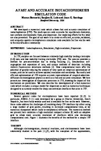
equations. A simple tail rotor model has been included which affects the pitching and yawing moment equilibrium. Details on the wind tunnel trim procedure employed in AVINOR can be found in Ref. 46. The trim equations need to be solved in terms of six trim variables, represented by the vector qt qt = {αR , θcoll , θ1c , θ1s , θ0t , φR }T ,

(79)

The equilibrium equations are formulated in the nonrotating, hub-fixed system, as shown schematically in Fig. 11. Note the flight path angle θFP is defined positive for descending flight, as shown in the figure. The drag Df is assumed to act parallel to the flight path. The six (3 force, 3 moments) propulsive trim equations for level and descending forward flight are arranged in the form20, 46 ft (qt ) = 0.

(80)

Let Rti be the vector of trim residuals at the trim condition qti at iteration i: ft (qti ) = Rti .

(81)

An iterative optimal control strategy is then used to reduce the value of Rti ; based on the minimization of the performance index:20 J = RT (82) ti Rti . This algorithm resembles a global feedback controller used for vibration reduction. The trim parameters at the ith iteration are then given by: qti = −T−1 (83) i Rti−1 + qti−1 , where Ti is a transfer matrix describing the sensitivities of trim residuals to changes in the trim variables: Ti =

∂Rti . ∂qt

(84)

Ti is computed using a finite difference scheme. III.D.

Aeroelastic Stability in Hover

The process for determining the hover stability of the blade is based on an extension of the method described in Ref. 22 in order to account for the RFA aerodynamic states.52 As described in Ref. 22, the hover stability analysis proceeds as follows: 1. The non-linear static equilibrium solution of the blade is found for a given pitch setting and uniform inflow, by solving a set of nonlinear algebraic equations. Note that uniform inflow is used only in the hover stability calculation. The forward flight analysis employs a free-wake model for inflow calculation.


2. The governing system of ordinary differential equations are linearized about the static equilibrium solution by writing perturbation equations and neglecting second-order and higher terms in the perturbed quantities. The linearized equations are rewritten in first-order state variable form. 3. The real parts of the eigenvalues of the first-order state variable matrix, λk = ζk + iωk , determine the stability of the system. If ζk ≤ 0 for all k, the system is stable. The governing aeroelastic equations in AVINOR are given by Eqs. 68 and 75, which are functions of blade response and the RFA aerodynamic states. Note that the states associated with the dynamic stall model can be neglected for hover analysis. Equations 68 and 75 represent the coupled set of ordinary differential equations that govern the rotor blade system. In the linearization process, perturbing Eq. 68 about the static equilibrium and neglecting the dynamic stall states and higher order terms gives ∂fb ∂fb ∂fb ∂fb ∆¨ y+ ∆y˙ + ∆y + ∆xa = 0 (85) ¨ q0 ∂y ∂ y˙ q0 ∂y q0 ∂xa q0 where q0 is the static equilibrium vector and is given by   y0   q0 =  y˙ 0  x˙ a0

(86)

The “0” subscript denotes static equilibrium solution. From Eq. 70, ∂gb ∂fb = ∂ y˙ q0 ∂ y˙ q0 ∂gb ∂fb = ∂y q0 ∂y q0 ∂fb ∂gb = . ∂xa q0 ∂xa q0

(87) (88) (89)

Substituting Eqs. 87 – 89 and Eq. 69 into Eq. 85 gives ∂gb ∂gb ∂gb [Mb ]q0 ∆¨ y+ ∆y˙ + ∆y + ∆xa = 0 ∂ y˙ q0 ∂y q0 ∂xa q0

(90)

Solving for ∆¨ y yields ∆¨ y = −M−1 b

∂gb ∂ y˙

∆y˙ − M−1 b

q0

∂gb ∂y

∆y − M−1 b

q0

∂gb ∂xa

∆xa .

(91)

q0

Similarly, Eq. 75 can be linearized, yielding ∂gaR ∂gaR ∂gaR ∆x˙ a = ∆y˙ + ∆y + ∆xa . ∂ y˙ q0 ∂y q0 ∂xa q0

(92)

Combining Eqs. 91 and 92 with the trivial perturbation equation ∆y˙ = ∆y˙ into first-order state space form gives z˙ = [A(q0 )]z (93) where



0h

 −1 ∂gb  b ∂y [A(q0 )] =  −M h i  ∂g aR

∂y

and

Ih

i

q0

q0

∂gb −M−1 b ∂ y˙ h i ∂gaR ∂ y˙



i q0

q0

−M−1 b h

0h

 ∂gb ∂xa

∂gaR ∂xa

i

i q0

   

(94)

q0



∆y   z ≡ ∆y =  ∆y˙  ∆xa The stability of the system is determined by the eigenvalues of A. 19 of 34 American Institute of Aeronautics and Astronautics

(95)

IV.

Postprocessing for Stress/Strain Recovery and Noise Prediction

The stress/strains and noise levels are calculated in postprocessing analyses because they do not affect the aeroelastic response solution. The solution of the 1-D strain measures are used to recover the 3-D blade stress/strain distribution at any instant in time. The acoustic analysis requires the unsteady pressure distribution over the surface of the blade as input. IV.A.

Stress/Strain Recovery

The YF/VABS strain field is recovered by substituting the 1-D strain measures and cross-sectional warping derivatives into Eqs. 8 – 11. Note that the contributions from in-plane warping are included in the YF/VABS strain field since UM/VABS accounts for in-plane warping. Stresses are obtained by substituting Eqs. 8 – 11 into Eq. 13. To facilitate the process of stress/strain recovery, UM/VABS outputs influence coefficients which multiply the 1-D strain measures to produce 3-D stress/strain distributions. The influence coefficients provided by UM/VABS are part of the solution of the 2-D cross-sectional problem. Using the 2-D strain influence coefficients and the AVINOR aeroelastic response solutions for the 1-D strain measures, the 3-D strain distribution at any instant in time, t, is given by 2 2 3 1 2 2 2 x2 + x3 κ1 7 6 7 6 0 7 6 7 6 0 7 6 (96) Γ (x1 , x2 , x3 , t) = [Π (x2 , x3 )] (x1 , t) + 6 7 7 6 0 7 6 7 6 0 5 4 0 T

where Π is a 6 × 6 matrix containing the strain influence coefficients, and = [γ11 2γ12 2γ13 κ1 κ2 κ3 ] . 2 Note that 21 x22 + x23 κ1 is added to Γ11 because of the contribution from the trapeze effect present in Eq. 8. In order to recover stresses, the elements of Π would be replaced with the stress influence coefficients. It should be noted that a higher order beam theory would be needed to impose zero beam strains at the root and therefore the current approach will only provide an accurate estimation of the cross-sectional stress distributions away from the boundary. IV.B.

Acoustic Model

The acoustic formulation for several helicopter noise codes is based on the Ffowcs Williams-Hawkings (FW-H) equation,53 which is written in an inhomogeneous wave equation form 1 ∂ 2 p0 ∂ ∂ ∂2 2 0 − ∇ p = [ρ v |∇f |δ(f ) − [l |∇f |σ(f )] − [Tij H(f )] 0 n i c2 ∂t2 ∂t ∂xi ∂xi ∂xj

(97)

The FW-H equation is derived by employing the conservation of mass and momentum for the fluid, which is valid for the entire three-dimensional space surrounding a moving body with arbitrary shape and motion. The rotational noise (thickness and loading noise) and BVI noise can be predicted with sufficient accuracy using the FW-H equation and neglecting the quadrupole source term. IV.B.1.

Unsteady Chordwise Pressure Calculation

The RFA approach was extended to calculate the chordwise pressure distribution, which is required in the acoustic calculation.21, 45, 46 In the extension of the RFA model for chordiwse pressure calculation the oscillatory pressure distribution obtained from the solution of Eq. 30 is saved; a separate RFA procedure similar to what is described in Section II.B.1 for sectional airloads computation is then carried out at each chordwise location, using the corresponding oscillatory pressure data.


A generalized pressure vector f p (t) is introduced: 

CP 1 CP 2 .. .

     p f =  CP i   ..  . CP n

      .    

(98)

This pressure vector represents the pressure coefficients on panels in the chordwise direction of the airfoil as shown in Fig. 12. The pressure computations introduce new aerodynamic states xpa ; however, this computation is performed separately after the aeroelastic response solution is obtained, thus the additional computational cost for the pressure computations is minimized and the original aeroelastic solution procedure is kept intact. As a means of validation, the force and moment coefficients obtained by integrating the pressure vector f p (t) are compared to the generalized force f (t) obtained from the original sectional RFA computation; typically with forty chordwise panels the sectional lift and moment coefficients can be reproduced within 5% when integrating pressure distribution over the chord.

Figure 12. Airfoil chordwise pressure distribution

The rational function approximations used to relate f p (t) to h(t) are similar to those that relate f (t) to h(t). The final state space equations for pressure distribution are: x˙pa (t)

=

f p (t)

=

U (t) ˙ R(M )xpa (t) + E(M )h(t), b 1 b ˙ p p p C0 (M )h(t) + C1 (M ) h(t) + D(M )xa (t) . U (t) U (t)

(99) (100)

These equations can be compared to Eqs. 40 and 41 for sectional airloads. Note the difference is that in the sectional airloads computations, the generalized motion vector h is unknown and is obtained from the coupled aeroelastic response solution; whereas h is known from the aeroelastic response solution and is available for the pressure computations in Eqs. 40 and 41, representing the fact that the pressure computations are decoupled from the aeroelastic solution procedure. IV.B.2.

Solution of the FW-H Equation

There exist a number of solutions to the FW-H equation,53 as documented in Ref. 54. One of Farassat’s solutions known as Formulation 1A55 has been implemented in several helicopter noise prediction codes due to its numerical efficiency. Using Green’s function of the wave equation in the unbounded domain δ(g)/4πr, where g = τ − t + r/c a retarded time solution to FW-H equation is obtained Z Z 1 ∂ ρ0 cvn + lr lr 4πp0 (x, t) = dS + dS 2 c ∂t f =0 r(1 − Mr ) ret f =0 r (1 − Mr ) ret 21 of 34 American Institute of Aeronautics and Astronautics

(101)

(102)

To improve the speed and accuracy of the solution, mathematical manipulations are carried out to move the time derivative inside the first integral of Eq. 102 by using the following relation 1 ∂ ∂ = (103) ∂t 1 − Mr ∂τ x

x ret

this yields Formulation 1A 1 = c

Z

1 + c Z 4πp0T (x, t) =

Z

4πp0L (x, t)

"

f =0

"

f =0

f =0

"

l˙i rî r(1 − Mr )2

#

Z dS + ret

f =0

lr (rM˙ i rî + cMr − cM 2 ) r2 (1 − Mr )3

l r − l i Mi r2 (1 − Mr )2

dS ret

#

ρ0 vn (rM˙ i rî + cMr − cM 2 ) r2 (1 − Mr )3

dS # dS

where

IV.B.3.

(104b)

ret

p0 (x, t) = p0L (x, t) + p0T (x, t) p0L , p0T , p0

(104a)

ret

(104c)

denotes the loading noise, thickness noise and overall noise, respectively.

BVI Noise Prediction

Blade-vortex interaction noise dominates the low speed descent flight regime, and is characterized by its impulsiveness and high intensity. The frequency content of BVI noise falls mostly in the mid-frequency range, which is most sensitive to human hearing. A widely accepted definition of BVI noise frequency range is the sum of 6th − 40th harmonics of blade passage frequency.49 Blade-vortex interaction noise is generated by unsteady pressure fluctuations on the blade induced by interaction with trailed vortices. More specifically, it originates primarily from the dipole or loading source term p0L in Eq. 104. Because of its impulsiveness, the prediction of BVI noise requires high fidelity blade surface pressure, with a typical resolution of less than 5◦ in azimuth. The pressure distribution, both chordwise and spanwise, is provided by the calculation described in Sec. IV.B.1. IV.B.4.

Modified WOPWOP Code

The acoustic model implemented in AVINOR is based on an extensively modified version of the helicopter aeroacoustic code WOPWOP56 developed at NASA Langley and combines it with the previously described aeroelastic analysis code. The WOPWOP code implements Farassat’s Formulation 1A (Eq. 104), and has been extensively validated57, 58 for helicopter noise predictions. The original version of WOPWOP requires blade harmonics and surface loading as input, which can be provided by either experiments or a suitable helicopter analysis code. A simple blade model based on the assumption of an offset hinged rigid blade has been used in the original WOPWOP code to generate the acoustic results. However, this simplified model is incompatible with the more realistic elastic blade described in Sec. II.A. In order to take into account the effects of blade flexibility, the blade dynamics in WOPWOP were replaced by the fully flexible blade model with partial span trailing edge flaps.21, 45 This was accomplished by discretizing the blade into a number of individual panels as shown in Fig. 13. The acoustic code then calculates the contribution from each panel, each having its own velocity, normal vector and pressure distribution. The time domain response of each of these panels was obtained from the aeroelastic response analysis. This information, together with the unsteady pressure distribution on the panel, serves as the basis of the acoustic computations. Unlike some computational studies performed with WOPWOP,59 a surface pressure distribution is used in the acoustic calculation, such that no reduction to a chordwise compact loading is made. Tail rotor or engine noise was not considered in this study. Furthermore, aerodynamic effects of the fuselage have been excluded, and thus the acoustic results represent the noise generated by the main rotor only.

V.

Active Control Algorithm

In AVINOR, active control of vibration, BVI noise, and rotor power is based on the higher-harmonic control (HHC) algorithm.6 The stability, robustness, and convergence properties of the algorithm and a number 22 of 34 American Institute of Aeronautics and Astronautics

Figure 13. Rigid and flexible blade representations

of variants were explored in Ref. 8. The algorithm is based on a linear, frequency domain representation of helicopter response to control inputs. The input harmonics to the ACF consist of a combination of flap deflection angles having frequencies of 2, 3, 4 and 5/rev. Thus, the total flap deflection is a combination of these contributions: 5 X δf (ψ) = [δN c cos(N ψ) + δN s sin(N ψ)] , (105) N =2

where δN c and δN s are the control amplitudes. The control strategy is based on the minimization of a performance index which is a quadratic function of the quantities that are being reduced, zk , and the control input amplitudes uk :6, 8 T JACF (zk , uk ) = zT k Qzk + uk Wu uk .

(106)

In the case of vibration reduction, T

zk,vr = [F4X F4Y F4Z M4X M4Y M4Z ]

.

(107)

For noise reduction, zk consists of the 6th – 17th harmonic components of BVI noise, T

zk,nr = [NH06 NH07 NH08 . . . NH17 ]

.

(108)

Although BVI noise is made up of the 6th – 40th harmonics, the 6th – 17th harmonics dominate the overall sound pressure level. Using only this range shortens the length of the vector zk,nr , which reduces the computational cost associated with the active control algorithm considerably. This implementation has been found to work well for BVI noise reduction.9 The noise components are measured at a microphone installed at the right rear landing skid, as shown in Fig. 14. For rotor power reduction, zk,pr = [JP ] . (109) where Ω JP = 2π

2π

Z

−MHZ (ψ) dψ ,

(110)

0

and MHZ is the total yawing moment about the hub. Equation 110 represents the instantaneous power required to drive the rotor at a constant angular velocity Ω averaged over one revolution. The effects of unsteadiness, compressibility, dynamic stall (if applicable), and the additional drag due to flap deflection is included in the calculation of MHZ . The engine must supply a torque equal to −MHZ in order to maintain 23 of 34 American Institute of Aeronautics and Astronautics

R

Carpet Plane

1.15R Onboard Microphones

Top View

Advancing Side

1

SKID1

0

Y

Y/R

-1

Retreating Side

X -2

-1

0

X/R

1

2

Figure 14. Carpet plane

a constant angular velocity. The relation for JP is a general expression which is valid for rotor blades with or without ACF’s. The optimal flap deflections are determined according to the control law described in Refs. 8 and 45, and can be written as −1 T uk+1 = − TT QT + Wu T (Qzk − QTuk ) (111) The relationship between the flap deflections and the quantities which need to be reduced is quantified by the transfer matrix T given by T = ∂zk /∂uk . The subscript k refers to the k th control update, reflecting the discrete-time nature of the controller; i.e. zk and uk are recalculated at specific times tk = k∆tk where ∆tk is the time interval between updates. Typically, ∆tk is set to 8 rotor revolutions, or settling revolutions, so that the system can reach a steady state. If the helicopter system cannot be perfectly represented by a linear model, the optimum control input will not be reached in a single step, and thus uk must be updated in order to converge to the optimal control input.8 Based on the implementations employed in Refs. 9 and 60, 8 control updates are used when considering BVI noise and vibration reduction, and 15 updates for vibration and power reduction in AVINOR. Traditionally, Eq. 111 is rewritten in iterative form as uk+1 = uk + ∆uk

(112)

In the relaxed HHC variant described in Ref. 8, a relaxation factor αr is introduced, resulting in uk+1 = uk + αr ∆uk

(113)

where 0 < αr < 1. This range has been shown to enhance the robustness of the control algorithm at the expense of convergence speed.8 In addition, the transfer matrix T is identified online following the adaptive HHC variant described in Ref. 8. The Wu matrix in Eq. 106 is used to enforce saturation limits on the flap deflections of |δf max | ≤ 4◦ , and is given by Wu = cwu I (114) where cwu is a scalar used to control the penalty on flap deflections and I is the identity matrix. If the flap deflections are overconstrained, then cwu is reduced and a new optimal control input is calculated. Similarly, cwu is increased if the flap deflections are underconstrained. Using the algorithm described in Ref. 61, cwu is automatically iterated upon until the flap deflections converge to within ±5% of δf max . To date, AVINOR has been used to study active control for BVI vibration and noise reduction, and vibration and power reduction at high advance ratios. 24 of 34 American Institute of Aeronautics and Astronautics

V.A.

BVI Induced Vibration and Noise Reduction

The vector zk is obtained by combining zk,vr and zk,nr as # " zk,vr . zk = zk,nr

(115)

In Eq. 106, Q is a diagonal weighting matrix. The weight matrices associated with vibration and noise reduction, Qvr and Qnr , are combined as " # (Wα ) · [Qvr ] 0 Q= , (116) 0 (1 − Wα ) · [Qnr ] where 0 ≤ Wα ≤ 1 is a user defined parameter which controls the emphasis of the controller. V.B.

Vibration and Power Reduction at High Advance Ratios

The vibration and power active control algorithm is formulated in a similar manner to the noise and vibration problem. The only differences are that zk,nr and Qk,nr would be replaced with zk,pr and Qk,pr in Eqs. 115 and 116 respectively.

VI.

Aeroelastic Tailoring of a Composite Rotor Blade for Vibration Reduction

In order to illustrate the usefulness of AVINOR combined with the UM/VABS composite sectional analysis for preliminary blade design, the problem of aeroelastically tailoring a blade for vibration reduction over the entire flight envelope is considered in this paper. The critical flight conditions for helicopter vibration occur at low advance ratios and high advance ratios. Vibration levels at low advance ratios are caused primarily by BVI and vibrations at high advance ratios are caused by dynamic stall. Therefore, a low vibration blade design must correspond to low vibration levels in both flight regimes. Since it is possible that the best blade design for one flight condition may not be the best for the other, this problem is treated as multi-objective function optimization problem in which the design corresponding to the best combination of vibration reduction at both advance ratios is sought. VI.A.

Formulation of the Blade Optimization Problem

The formulation of the blade optimization problem in forward flight consists of several ingredients: the objective function, design variables, and constraints. The mathematical formulation of the optimization is stated as: Find the vector of design variables D which minimizes the objective function, i.e. J(D) → min. The vibration objective function consists of a combination of the Nb /rev oscillatory hub shears and moments. For a four bladed rotor, the vibration objective function is given by p p J = KS (F4X )2 + (F4Y )2 + (F4Z )2 + KM (M4X )2 + (M4Y )2 + (M4Z )2 (117) where KS and KM are appropriately selected weighting factors. Equation 117 is evaluated in the BVI and dynamic stall regimes, resulting in the objective functions JBVI and JDS . The vector of cross-sectional design variables D consists of the ply angles in the 7 walls depicted in Fig. 15. The blade is assumed to have uniform spanwise properties, thus there are a total of 7 design variables in this problem. The design variables have side constraints to prevent them from reaching impractical values; these are stated as (L) (U ) Dj ≤ D ≤ Dj , j = 1, 2, . . . , Ndv . (118) In addition, behavior constraints are placed on the aeroelastic stability margins and are stated as: gk (D) = ζk + (ζk )min ≤ 0,

k = 1, 2, . . . , Nm

(119)

where Nm is the number of normal modes, ζk is the real part of the hover stability eigenvalue for the k th mode, and (ζk )min is the minimum acceptable damping level for the kth mode.


xv E-glass S-glass D1 D2 D3 D4 D5 D6

1.8 mm 5.2 mm 5.4 mm

D7

Figure 15. Composite blade cross-section.

The second type of behavior constraints are the constraints placed on the maximum blade strains, ¯ 11 − Γ ¯ T11 ≤ 0 , g11,T = Γ T

(120)

¯ 22 − Γ ¯ 22 ≤ 0 , g22,T = Γ

(121)

¯ C11 − Γ ¯ 11 ≤ 0 , g11,C = Γ

(122)

¯ C22 − Γ ¯ 22 ≤ 0 , g22,C = Γ

(123)

¯ 12 | − Γ ¯ S12 ≤ 0 . g12 = |2Γ

(124)

In Eqs. 120 – 124, the strain components correspond to a coordinate system aligned with the fiber angles; ¯ 11 is in the direction of the fiber axis, Γ ¯ 22 is the transverse strain component, and Γ ¯ 22 is the shear i.e. Γ ¯T , Γ ¯ C , and Γ ¯S strain. The maximum allowable strains in tension, compression, and shear are given by Γ 12 ii ii respectively. Equations 120 – 124 denote that the maximum blade strains at any location on the blade and at any time must be less than allowable quantities. VI.B.

Surrogate-Based Optimization

The blade optimization problem is solved using a surrogate-based approach.62, 63 To facilitate a global search of the design space in a reasonable amount of time, it is necessary to use global approximation, or surrogate methods, where the “true” objective function and expensive constraints are replaced with smooth functional relationships of acceptable accuracy that can be evaluated quickly. To construct the surrogates, the objective function and expensive constraints must first be evaluated over a set of design points. The surrogates are then generated by fitting the initial data points. In this process, function evaluations based on expensive helicopter simulations are needed to form the approximations. However, this initial investment of computer time is relatively small compared to global searches based on non-surrogate optimization methods. In this study, the objective function given by Eq. 117 in both flight regimes and the maximum strain constraints


Rotor Data R = 4.91 m Nb = 4 βp = 2.5◦ θpt = −8◦ σ = 0.07 XF A = 0.0 XF C = 0.0 Cdf = 0.01

Ω = 425 rpm c = 0.05498R Cdo = 0.01 CW = 0.005 CT /σ = 0.0714 ZF A = 0.3 ZF C = 0.3

BVI Flight Condition µ = 0.15

αd = 6.5◦

Dynamic Stall Flight Condition µ = 0.35

αd = 0◦

Table 1. Rotor and helicopter parameters

given by Eqs. 120 – 124 are replaced by surrogates. The surrogate-based optimization approach employed in this study is based on a modified version of the Efficient Global Optimization (EGO) algorithm.64 The EGO algorithm is modified for multi-objective function optimization using the approach described in Refs. 12 and 65.

VII.

Results

The helicopter configuration and flight condition parameters used in all the computations are given in Table 1. The simulations are conducted for two flight conditions – low speed forward flight where high vibration levels due to blade-vortex interaction (BVI) are encountered, and a high speed forward flight condition where high vibrations are caused by dynamic stall. Figure 11 illustrates the geometrical data needed for the propulsive trim calculation used in this study. In this study, 8 modes are used in the modal reduction: the first 3 flap modes, first 2 lead-lag modes, the first 2 torsional modes, and the first axial mode. VII.A.

Generation of a Baseline Design

In order to determine the quality of the aeroelastically tailored blade designs, it is necessary to have a baseline blade model for comparisons. The goal in generating a baseline model was to reproduce as closely as possible a model resembling an MBB BO-105 rotor blade that has been used in previous structural optimization studies.11, 12 The MBB BO-105 is generally considered to have good vibration characteristics. Specifically, the following characteristics were required: 1. Hingeless blade with uniform spanwise properties and the same mass as the MBB BO-105 model. 2. A design that is aeroelastically stable in hover. 3. Fundamental flap, lag, and torsional frequencies similar to the MBB BO-105 model. 4. For the BVI and dynamic stall flight conditions, maximum compressive strain amplitudes less than 5, 000 microstrain, and maximum tensile and shears strains less than 10, 000 microstrain. In order to obtain these characteristics, a genetic algorithm optimizer from the iSIGHT software package66 was used to select cross-sectional parameters until a suitable design was found. Referring to Fig 15, the genetic algorithm operated on the following design variables: the fiber angles in the 7 composite plies (D1 . . . D7 ), and the chordwise location of the vertical wall (xv ). The baseline cross-sectional parameters


Table 2. Baseline cross-sectional parameters

Parameters

Value

D1 D2 D3 D4 D5 D6 D7 xv

79◦ 24◦ −10◦ −24◦ 7◦ −70◦ −79◦ 66.6 mm

Table 3. Fundamental frequencies of the baseline design and the MBB BO-105

Mode

Baseline Design Values

MBB BO-105 Vales

ωL1 ωF 1 ωT 1

0.729 /rev 1.033 /rev 3.261 /rev

0.729 /rev 1.125 /rev 3.263 /rev

selected by the genetic algorithm are provided in Table 2, and the fundamental frequencies of the resulting design are given in Table 3. The elastic axis of the baseline design is 2% of the chord in front of the quarter chord position. The mass of the baseline cross-section was 2.69 kg/m. Since the mass of the MBB BO-105 model is 5.57 kg/m, 2.88 kg/m of non-structural mass was added to the baseline design. The non-structural mass was placed at a chordwise location such that the c.g. coincides with the quarter chord. The baseline design maximum strains at the BVI and dynamic stall flight conditions are provided in Table 4. VII.B.

Optimization Parameters

In addition to the data in Table 1, additional information is required to represent the objective function, constraints, and the finite element discretization of the blade. The weighting factors in the objective function, KS and KM , are selected to be 1. These weighting factors result in an objective function which represents the sum of the 4/rev oscillatory hub shear resultant and the 4/rev oscillatory hub moment resultant in the hub-fixed non-rotating frame. For this study, the following side constraints are enforced: −90◦ ≤ Di ≤ 90◦ ,

i = 1, 2, . . . , 7.

(125)

For the aeroelastic stability constraints given by Eq. 119, the minimum acceptable damping for all modes, (ζk )min , is chosen to be 0.01.22, 23 Additionally, the constraints are modified for the 2nd lag mode, which can sometimes be slightly unstable.67 To prevent this situation, a small amount of structural damping is added to this mode. A small amount of damping is almost always present in actual blade configurations, and therefore adding it in trend type studies such as this paper has little significance. For this study, 0.5% structural damping is added to stabilize the 2nd lag mode of the baseline blade. The maximum strain components are constrained to be less than the baseline design values unless stated otherwise. VII.C.

Multi-objective Function Optimization Results

The results obtained from the multi-objective surrogate-based optimization approach described in Sec. VI.B are presented in this section. Table 5 lists the designs corresponding to the best trade-offs between vibration reduction in the BVI regime and vibration reduction in the dynamic stall regime when no maximum strain constraints are enforced. The designs correspond to 53 − 37% reduction of BVI induced vibrations compared 28 of 34 American Institute of Aeronautics and Astronautics

Table 4. Maximum strains in forward flight for the baseline blade model

Strain Component

BVI Condition (microstrain)

Dynamic Stall Condition (microstrain)

¯ 11 (compression) Γ ¯ 11 (tension) Γ ¯ Γ22 (compression) ¯ 22 (tension) Γ ¯ 12 2Γ

-1700 4900 -1600 4500 7500

-1800 5200 -1600 4700 8200

Table 5. Best trade-off designs (no maximum strain constraints)

D1

D2

D3

D4

D5

D6

D7

ωL1 (/rev)

ωF 1 (/rev)

ωT 1 (/rev)

% Vibration Reduction (BVI)

% Vibration Reduction (Dynamic Stall)

−48◦ −49◦ −56◦ −49◦

0◦ 14◦ 62◦ 89◦

14◦ 9◦ −30◦ −4◦

5◦ −14◦ −4◦ −24◦

22◦ 2◦ −52◦ 2◦

−36◦ −46◦ −11◦ −46◦

51◦ −68◦ 44◦ −67◦

0.657 0.655 0.641 0.638

1.031 1.031 1.029 1.029

3.820 3.847 3.865 3.844

53 51 37 37

38 40 50 60

to the baseline blade, and 38 − 60% reduction in the dynamic stall regime. As in Ref. 12, the best design for one flight condition is not the best for the other. The best trade-off designs when constraining the maximum strains to be less than the baseline values are given in Table 6. With the constraints applied to the strains, the maximum amount of vibration reduction under dynamic stall conditions is 13% less than the unconstrained case, while the maximum vibration reduction at low advance ratios is unchanged compared to the unconstrained case. Therefore, the strain constraint is more active for the vibration reduction objective function at high advance ratios. The effect of the strain constraint is illustrated in Fig. 16 in which the levels of vibration reduction corresponding to the best trade-off designs are plotted (i.e. the Pareto front). The constrained Pareto front has a much stronger slope than the unconstrained front. This means that significant penalties in BVI induced vibration must be tolerated in order to achieve relatively small improvements in vibration levels at high advance ratios. For instance, compared to the first design in Table 6, selecting the third design would mean giving up 25% vibration reduction in the BVI regime in order to achieve an additional 5% vibration reduction in the dynamic stall regime. Therefore, it is unlikely that a blade designer would select any of the last three designs in Table 6 as the best trade-off design. The non-zero cross-sectional parameters calculated by UM/VABS (see Eq. 20) for the first trade-off design in Table 6 and the baseline model are listed in Table 7. Note that there is no flap-bending/torsion coupling (H45 in Eq. 20) introduced through material anisotropy. It has been shown computationally29, 30 and experimentally35 that flap-bending/torsion coupling can have a beneficial effect on vibratory loads. The results in this study indicate that elastic couplings in addition to flap-bending/torsion can also lead to lower vibration levels. A comparison of the vibratory hubloads corresponding to the baseline design and the first trade-off design in Table 6 is provided in Fig. 17. The trade-off design reduces the longitudinal and lateral shears in the BVI regime by 27 − 37%. However, most of the reduction in the vibration objective function is achieved by the 95% reduction of the vertical shear, which is the largest vibratory component in the BVI regime. In contrast, the mechanism for reducing the dynamic stall objective function is achieved by a 19 − 36% reduction of all ¯ 11 , Γ ¯ 22 , and 2Γ ¯ 12 are reduced by 12%, three shears. Furthermore, the maximum tensile and shear strains, Γ 54%, and 11% respectively. Thus, aeroelastic tailoring led to a design corresponding to significantly reduced vibration and reduced maximum strain levels compared to a baseline design. These results illustrate the usefulness of AVINOR for preliminary design studies.


Table 6. Best trade-off designs (maximum strains constrained)

D1

D2

D3

D4

D5

D6

D7

ωL1 (/rev)

ωF 1 (/rev)

ωT 1 (/rev)

% Vibration Reduction (BVI)

% Vibration Reduction (Dynamic Stall)

−48◦ −49◦ −45◦ −47◦ −48◦

0◦ 14◦ −12◦ −9◦ −9◦

14◦ 9◦ 9◦ 9◦ 9◦

5◦ −14◦ 4◦ −2◦ −2◦

22◦ 2◦ −7◦ −89◦ −77◦

−36◦ −46◦ −29◦ −33◦ −33◦

51◦ −68◦ 55◦ 50◦ 50◦

0.657 0.655 0.656 0.657 0.658

1.031 1.031 1.031 1.031 1.031

3.820 3.847 3.855 3.841 3.834

53 51 28 26 22

38 40 43 46 47

Unconstrained Pareto front

50%

Constrained Pareto front

Reduction in BVI Objective Function

60%

40%

30%

20%

10%

0% 30%

35%

40%

45%

50%

55%

60%

65%

Reduction in Dynamic Stall Objective Function Figure 16. Unconstrained and Constrained Best Trade-offs (i.e. the Pareto front)

VIII.

Conclusions

A description of the AVINOR rotor blade aeroelastic response simulation code is provided in this paper. AVINOR is of suitable fidelity and computational efficiency to be useful for preliminary design studies. The applicability of AVINOR for rotor blade design was illustrated by considering the problem of aeroelastically tailoring a composite rotor blade for reduced vibration over the entire flight envelope. Using UM/VABS as the cross-sectional analysis, a design corresponding to reduced vibration and maximum strains compared to a baseline blade was obtained via aeroelastic tailoring. The principal results from the aeroelastic tailoring study are summarized below. 1. Enforcing a constraint on the maximum beam strains did not affect the amount of vibration reduction that could be achieved in the BVI regime, but limited the improvement that could be achieved in the dynamic stall regime. 2. Utilizing a surrogate-based approach led to a trade-off design corresponding to 53% vibration reduction compared to a baseline blade at low advance ratios where BVI is the dominant source of vibration, and 38% vibration reduction at high advance ratios where dynamic stall is the source of high vibration. ¯ 11 , Γ ¯ 22 , and 2Γ ¯ 12 , were reduced by 12%, 54%, Furthermore, the maximum tensile and shear strains, Γ and 11% respectively.


Cross-sectional Parameter

Baseline

Trade-off Design

H11 H13 H14 H16 H22 H25 H33 H34 H36 H44 H46 H55 H66

3.74 × 107 N −9.81 × 104 N −4.37 × 104 N-m 6.90 × 105 N-m 4.15 × 106 N 1.97 × 104 N-m 3.75 × 105 N 1.82 × 103 N-m 2.90 × 104 N-m 2.80 × 103 N-m2 −2.31 × 103 N-m2 4.01 × 103 N-m2 2.16 × 105 N-m2

3.39 × 107 N 4.06 × 104 N 4.07 × 104 N-m 1.01 × 105 N-m 7.73 × 106 N −1.32 × 104 N-m 6.62 × 105 N −6.47 × 102 N-m −1.62 × 104 N-m 4.35 × 103 N-m2 7.43 × 101 N-m2 3.41 × 103 N-m2 1.49 × 105 N-m2

0.0016

Nondimensional 4/rev Vibratory Loads

Nondimensional 4/rev Vibratory Loads

Table 7. Non-zero cross-sectional parameters corresponding to the baseline and trade-off designs

Trade-off Design Baseline

0.0012

0.0008

0.0004

0

0.0036

Trade-off Design Baseline

0.0027

0.0018

0.0009

0

F4X

F4Y

F4Z

M4X

M4Y

M4Z

F4X

BVI regime, µ = 0.15

F4Y

F4Z

M4X

M4Y

M4Z

Dynamic stall regime, µ = 0.35

Figure 17. Vibratory hubloads in the BVI and dynamic stall flight regimes

3. Significant levels of vibration reduction were achieved without flap-bending/torsion composite coupling, which has been noted in previous studies to have a beneficial effect on vibratory loads. The results in this study indicate that elastic couplings in addition to flap-bending/torsion can also lead to lower vibration levels.

Acknowledgments This research was supported in part by an NSF sponsored AGEP postdoctoral fellowship for B. Glaz. Partial support from the Center for Rotorcraft Innovation under WBS 2007-B-01-01.2-A17, as well as the Vertical Lift Research Center of Excellence (VLRCOE) sponsored by the NRTC with Dr. M. Rutkowski as grant monitor is also hereby acknowledged.

References 1 Davis, M. W. and Weller, W. H., “Helicopter Rotor Dynamics Optimization with Experimental Verification,” Journal of Aircraft, Vol. 28, No. 1, 1991, pp. 38 – 48. 2 Weller, W. H. and Davis, M. W., “Wind Tunnel Tests of Helicopter Blade Designs Optimized for Minimum Vibrations,”


Journal of the American Helicopter Society, Vol. 34, No. 3, 1989, pp. 40 – 50. 3 Young, D. K. and Tarzanin, F. J., “Structural Optimization and Mach Scale Test Validation of a Low Vibration Rotor,” Journal of the American Helicopter Society, Vol. 38, No. 3, 1993, pp. 83 – 92. 4 Friedmann, P. P. and Millott, T. A., “Vibration Reduction in Rotorcraft Using Active Control: A Comparison of Various Approaches,” Journal of Guidance, Control, and Dynamics, Vol. 18, No. 4, July-August 1995, pp. 664–673. 5 Chopra, I., “Status of Application of Smart Structures Technology to Rotorcraft Systems,” Journal of the American Helicopter Society, Vol. 45, No. 4, Oct. 2000, pp. 228–252. 6 Johnson, W., Self-Tuning Regulators for Multicyclic Control of Helicopter Vibrations, NASA Technical Paper 1996, 1982. 7 Millott, T. A. and Friedmann, P. P., Vibration Reduction in Helicopter Rotors Using an Actively Controlled Partial Span Trailing Edge Flap Located on the Blade, NASA CR 4611, June 1994. 8 Patt, D., Liu, L., Chandrasekar, J., Bernstein, D. S., and Friedmann, P. P., “Higher-Harmonic-Control Algorithm for Helicopter Vibration Reduction Revisited,” Journal of Guidance, Control, and Dynamics, Vol. 28, No. 5, September-October 2005, pp. 918–930. 9 Patt, D., Liu, L., and Friedmann, P. P., “Simultaneous Vibration and Noise Reduction in Rotorcraft Using Aeroelastic Simulation,” Journal of the American Helicopter Society, Vol. 51, No. 2, 2006, pp. 127–140. 10 Liu, L., Friedmann, P. P., Kim, I., and Bernstein, D. S., “Rotor Performance Enhancement and Vibration Reduction in Presence of Dynamic Stall Using Actively Controlled Flaps,” Journal of the American Helicopter Society, Vol. 53, No. 4, Oct. 2008, pp. 338 – 351. 11 Glaz, B., Goel, T., Liu, L., Friedmann, P. P., and Haftka, R. T., “Multiple-Surrogate Approach to Helicopter Rotor Blade Vibration Reduction,” AIAA Journal, Vol. 47, No. 1, Jan. 2009, pp. 271–282. 12 Glaz, B., Friedmann, P. P., and Liu, L., “Helicopter Vibration Reduction throughout the Entire Flight Envelope Using Surrogate-Based Optimization,” Journal of the American Helicopter Society, Vol. 54, No. 1, Jan. 2009. 13 Glaz, B., Friedmann, P. P., and Liu, L., “Vibration and Noise Reduction of Helicopter Rotors Using an Active/Passive Approach,” American Helicopter Society’s Specialist’s Conference on Aeromechanics, San Francisco, CA, Jan. 23 – 25 2008. 14 Glaz, B., Friedmann, P. P., and Liu, L., “Vibration Reduction and Performance Enhancement of Helicopter Rotors Using an Active/Passive Approach,” 49th AIAA/ASME/ASCHE/AHS/ASC Structures, Structural Dynamics & Materials Conference, Schaumburg, IL, April 7 – 10 2008, pp. 1 – 18, AIAA Paper 2008-2178. 15 Myrtle, T. F. and Friedmann, P. P., “Application of a New Compressible Time Domain Aerodynamic Model to Vibration Reduction in Helicopters Using an Actively Controlled Flap,” Journal of the American Helicopter Society, Vol. 46, No. 1, Jan. 2001, pp. 32–43. 16 Petot, D., “Differential Equation Modeling of Dynamic Stall,” La Recherche A´ erospatiale, Vol. 5, 1989, pp. 59–71. 17 Depailler, G. and Friedmann, P. P., “Reductions of Vibrations Due to Dynamic Stall in Helicopters Using an Actively Controlled Flap,” Proceedings of the 43rd AIAA/ASME/ASCE/AHS/ACS Structures, Structural Dynamics and Materials Conference, Denver, CO, April 2002, AIAA Paper No. 2002-1431. 18 Johnson, W., CAMRAD/JA - A Comprehensive Analytical Model of Rotorcraft Aerodynamics and Dynamics, Vol I. Theory Manual, Johnson Aeronautics, Palo Alto, CA, 1988. 19 Johnson, W., CAMRAD/JA - A Comprehensive Analytical Model of Rotorcraft Aerodynamics and Dynamics, Vol II. Users’ Manual, Johnson Aeronautics, Palo Alto, CA, 1988. 20 de Terlizzi, M., Blade Vortex Interaction and Its Alleviation Using Passive and Active Control Approaches, Ph.D. thesis, UCLA, 1999. 21 Patt, D., Liu, L., and Friedmann, P. P., “Rotorcraft Vibration Reduction and Noise Prediction Using a Unified Aeroelastic Response Simulation,” Journal of the American Helicopter Society, Vol. 50, No. 1, January 2005, pp. 95–106. 22 Yuan, K. A. and Friedmann, P. P., Aeroelasticity and Structural Optimization of Composite Helicopter Rotor Blades with Swept Tips, NASA CR 4665, May 1995. 23 Yuan, K. A. and Friedmann, P. P., “Structural Optimization for Vibratory Loads Reduction of Composite Helicopter Rotor Blades with Advanced Geometry Tips,” Journal of the American Helicopter Society, Vol. 43, No. 3, July 1998, pp. 246– 256. 24 Cesnik, C. E. S. and Hodges, D. H., “VABS: A New Concept for Composite Rotor Blade Cross-Sectional Modeling,” Journal of the American Helicopter Society, Vol. 42, No. 1, Jan. 1997, pp. 27–38. 25 Hodges, D. H., Nonlinear Composite Beam Theory, AIAA, Reston, VA, 2006. 26 Palacios, R. and Cesnik, C. E. S., “Cross-Sectional Analysis of Non-Homogeneous Anisotropic Active Slender Structures,” AIAA Journal, Vol. 43, No. 12, December 2005, pp. 2624–2638. 27 Friedmann, P. P., Glaz, B., and Palacios, R., “A Moderate Deflection Composite Helicopter Rotor Blade Model with an Improved Cross-Sectional Analysis,” International Journal of Solids and Structures, Vol. 46, No. 10, May 2009, pp. 2186 – 2200. 28 Yu, W., Volovoi, V. V., Hodges, D. H., and Hong, X., “Validation of the Variational Asymptotic Beam Sectional Analysis,” AIAA Journal, Vol. 40, No. 10, Oct. 2002, pp. 2105–2112. 29 Ganguli, R. and Chopra, I., “Aeroelastic Optimization of a Helicopter Rotor with Two-Cell Composite Blades,” Journal of the American Helicopter Society, Vol. 34, No. 4, April 1996, pp. 835 – 841. 30 Ganguli, R. and Chopra, I., “Aeroelastic Optimization of a Helicopter Rotor to Reduce Vibration and Dynamic Stresses,” Journal of the Aircraft, Vol. 12, No. 4, July – Aug. 1996, pp. 808 – 815. 31 Smith, E. C. and Chopra, I., “Aeroelastic Response, Loads, and Stability of a Composite Rotor in Forward Flight,” AIAA Journal, Vol. 31, No. 7, Jan. 1993, pp. 1265 – 1274. 32 Ganguli, R., “Optimal Design of a Low Vibration Helicopter Rotor Using Response Surface Approximation,” Journal of Sound and Vibration, Vol. 258, No. 2, 2002, pp. 327–344. 33 Murugan, S. and Ganguli, R., “Aeroelastic Stability Enhancement and Vibration Supression in a Composite Helicopter Rotor,” Journal of Aircraft, Vol. 42, No. 4, July-August 2005, pp. 1013–1024.


34 Cesnik, C. E. S., Mok, J., Morillo, J. A., and Parikh, A. S., “Design Optimization of Active Twist Rotor Blades,” Proceedings of the 30th European Rotorcraft Forum, Marseille, France, September 2004. 35 Bao, J., Nagaraj, V. T., Chopra, I., and Bernhard, P. F., “Wind Tunnel Test of Five Sets of Mach Scale Composite Tailored Rotor with Flap-Bending/Torsion Couplings for Vibration Reduction,” Journal of the American Helicopter Society, Vol. 53, No. 3, July 2008, pp. 215 – 225. 36 Yu, W., Hodges, D. H., Volovoi, V. V., and Cesnik, C. E. S., “On Timoshenko-like Modeling of Initially Curved and Twisted Composite Beams,” International Journal of Solids and Structures, Vol. 39, No. 19, Sept. 2002, pp. 5101–5121. 37 Hodges, D. H., Saberi, H., and Ormiston, R. A., “Development of Nonlinear Beam Elements for Rotorcraft Comprehensive Analyses,” Journal of the American Helicopter Society, Vol. 52, No. 1, Jan. 2007, pp. 36–48. 38 Hodges, D. H. and Yu, W., “A Rigorous, Engineer-friendly Approach for Modeling Realistic, Composite Rotor Blades,” Wind Energy, Vol. 10, 2007, pp. 179–193. 39 Depailler, G. and Friedmann, P. P., “Alleviation of Dynamic Stall Induced Vibrations Using Actively Controlled Flaps,” 58th Annual Forum of the American Helicopter Society, Montreal, Canada, June 2002. 40 Rogers, K. L., Airplane Math Modeling Methods for Actively Control Design, AGARD-CP-228, August 1977. 41 Rodden, W. P. and Albano, E., “A Doublet-Lattice Method for Calculating Lift Distributions on Oscillating Surfaces in Subsonic Flows,” AIAA Journal, Vol. 7, 1969, pp. 279–285. 42 Bisplinghoff, R. L., Ashley, H., and Halfman, R., Aeroelasticity,, Addison-Wesley, 1955. 43 Depailler, G., Alleviation of Dynamic Stall Induced Vibrations on Helicopter Rotors Using Actively Controlled Flaps, Ph.D. thesis, University of Michigan, Ann Arbor, 2002. 44 Leishman, J. G., Principles of Helicopter Aerodynamics, Cambridge University Press, Second ed., 2006. 45 Patt, D., Simultaneous BVI Noise, and Vibration Reduction in Rotorcraft using Actively-Controlled Flaps and Including Performance Considerations, Ph.D. thesis, University of Michigan, 2004. 46 Liu, L., BVI Induced Vibration and Noise Alleviation by Active and Passive Approaches, Ph.D. thesis, University of Michigan, 2005, Aerospace Engineering. 47 Scully, M. P., Computation of Helicopter Rotor Wake Geometry and its Influence on Rotor Harmonic Airloads, Ph.D. thesis, Aeroelastic Research Laboratory, Massachusetts Institute of Technology, 1975. 48 Splettstoesser, W., Seelhorst, U., Wagner, W., Boutier, A., Micheli, F., Mercker, E., and Pengel, K., “Higher Harmonic Control Aeroacoustic Rotor Test (HART) - Test Documentation and Representative Results,” Report IB 129-95/28 and appendices, DLR, Dec. 1995. 49 Splettstoesser, W., Kube, R., Wagner, W., Seelhorst, U., Boutier, A., Micheli, F., Mercker, E., and Pengel, K., “Key Results From a Higher Harmonic Control Aeroacoustic Rotor Test (HART),” Journal of the American Helicopter Society, Vol. 42, No. 1, Jan. 1997, pp. 58–78. 50 Rahier, G. and Delrieux, Y., “Blade-Vortex Interaction Noise Prediction Using a Rotor Wake Roll-Up Model,” Journal of Aircraft, Vol. 34, No. 4, July-August 1997, pp. 522–530. 51 Shampine, L. F., Numerical Solution of Ordinary Differential Equations, Chapman and Hall, New York, 1994. 52 Glaz, B., Friedmann, P. P., and Liu, L., “Surrogate Based Optimization of Helicopter Rotor Blades for Vibration Reduction in Forward Flight,” Structural and Multidisciplinary Optimization, Vol. 35, No. 4, April 2008, pp. 341 – 363. 53 Ffowcs Williams, J. E. and Hawkings, D. L., “Sound Generation by Turbulence and Surfaces in Arbitrary Motion,” Philosophical Transactions of Royal Soc. London, Series A, Vol. 264, No. 1151, May 1969, pp. 321–342. 54 Farassat, F., “Linear Acoustic Formulas for Calculation of Rotating Blade Noise,” AIAA Journal, Vol. 19, No. 9, Sept. 1981. 55 Farassat, F. and Succi, G. P., “The Prediction of Helicopter Rotor Discrete Frequency Noise,” Vertica, Vol. 7, No. 4, May 1983, pp. 309–320. 56 Brenter, K., A Computer Program Incorporating Realistic Blade Motions and Advanced Acoustic Formulation, NASA Technical Memorandum, Vol. 87721 1986. 57 Brentner, K. S. and Farassat, F., “Helicopter Noise Prediction: The Current Status and Future Direction,” Journal of Sound and Vibration, Vol. 170(1), 1994, pp. 79–96. 58 Brentner, K. S. and Farassat, F., “Modeling Aerodynamically Generated Sound of Helicopter Rotors,” Progress in Aerospace Sciences, Vol. 39, No. 2–3, February–April 2003, pp. 83–120. 59 Boyd, D. D., Brooks, T. F., Burley, C. L., and Jolly, J. R., “Aeroacoustic Codes for Rotor Harmonic and BVI Noise Camrad.Mod1/HIRES,” Journal of the American Helicopter Society, Vol. 45, No. 2, April 2000, pp. 63–89. 60 Liu, L., Friedmann, P. P., Kim, I., and Bernstein, D. S., “Vibration Reduction and Performance Enhancement in Rotorcraft Using Active Flaps at High Advance Ratios,” 47th AIAA/ASME/ASCHE/AHS/ASC Structures, Structural Dynamics & Materials Conference, Newport, RI, May 1-4 2006, pp. 1–21, AIAA Paper 2006-1861. 61 Cribbs, R. and Friedmann, P. P., “Actuator Saturation and Its influence on Vibration Reduction by Actively Controlled Flaps,” Proceedings of the 42nd AIAA/ASME/ASCE/AHS/ACS Structures, Structural Dynamics and Materials Conference, Seattle, WA, April 2001, AIAA Paper No. 2001-1467. 62 Queipo, N. V., Haftka, R. T., Shyy, W., Goel, T., Vaidyanathan, R., and Tucker, P. K., “Surrogate-Based Analysis and Optimization,” Progress in Aerospace Sciences, Vol. 41, 2005, pp. 1–28. 63 Forrester, A. I. J., S´ obester, A., and Keane, A. J., Engineering Design via Surrogate Modelling: A Practical Guide, AIAA, Reston, VA, 2008. 64 Jones, D. R., Schonlau, M., and Welch, W. J., “Efficient Global Optimization of Expensive Black-Box Functions,” Journal of Global Optimization, Vol. 13, 1998, pp. 455–492. 65 Glaz, B., Active/Passive Optimization of Helicopter Rotor Blades for Improved Vibration, Noise, and Performance Characteristics, Ph.D. thesis, University of Michigan, 2008, Aerospace Engineering.


66 Koch, P. N., Evans, J. P., and Powell, D., “Interdigitation for Effective Design Space Exploration using iSIGHT,” Structural and Multidisciplinary Optimization, Vol. 23, No. 2, 2002, pp. 111–126. 67 Friedmann, P. P. and Straub, F., “Application of the Finite Element Method to Rotary-Wing Aeroelasticity,” Journal of the American Helicopter Society, Vol. 25, No. 1, January 1980, pp. 36 – 44.


The AVINOR Aeroelastic Simulation Code and Its ... - CiteSeerX

The AVINOR Aeroelastic Simulation Code and Its ... - CiteSeerX

Suggest Documents

Simulation Study of Impact of Aeroelastic Characteristics ... - CiteSeerX

Environmental report 2013 - Avinor

Experiences in Aeroelastic Simulation Practices - Core

Nonlinear Aeroelastic Analysis, Flight Dynamics, and ... - CiteSeerX

Simulation and Flight Control of an Aeroelastic Fixed Wing Micro ...

Aeroelastic modeling for the FIT team F/A-18 simulation

The ORBIT Simulation Code: Benchmarking and Applications

Development of an Aeroelastic Code Based on an Euler/Navier ...

Numerical simulation of aeroelastic instabilities of elementary bridge ...

Static aeroelastic simulation of military aircraft configuration in ... - Core

Cisneros' Code-Mixed Narrative and its Implications for ... - CiteSeerX

Cisneros' Code-Mixed Narrative and its Implications for ... - CiteSeerX

MOLECULAR DYNAMICS SIMULATION AND ITS

Aeroelastic Control Using Multiple Control Surfaces - CiteSeerX

Aeroelastic simulation of flexible flapping wing based on structural ...

Time-accurate simulation of helicopter rotor flows including aeroelastic

Aeroelastic flutter of feathers, flight and the

Analytical aeroelastic stability considerations and

Output Feedback Control of the Nonlinear Aeroelastic ... - CiteSeerX

Code Generation for Simulation and Control ...

Magnetohydrodynamic Simulation Code CANS+: Assessments and ...

A FAST AND ACCURATE ISOTACHOPHORESIS SIMULATION CODE

The Particle Accelerator Simulation Code PyORBIT - Core

Cracking the Code - CiteSeerX