The Lagrange Interpolation Polynomial for Neural Network Learning

IJCSNS International Journal of Computer Science and Network Security, VOL.11 No.3, March 2011

255

The Lagrange Interpolation Polynomial for Neural Network Learning Khalid Ali Hussien Mustansiriyah University, Educational College, Baghdad, Iraq Abstract One of the methods used to find this polynomial is called the Lagrange method of interpolation. In this research, the Lagrange interpolation method was used in a new neural network learning by develops the weighting calculation in the back propagation training. This proposed developing decrease the learning time with best classification operation results. Also, the Langrage interpolation polynomial was used to process the image pixels and remove the noise the image. This interpolation gives the effective processing in removing the noise and error in the image layers. One of the advantages of this method is reduce the noise to minimum value by replacing the noisy pixels (detected by Lagrange Back propagation Neural Network LBPNN) by results calculated by the Lagrange interpolation with high speed processing and best RMSE results.

Keyword: Interpolation polynomial, Lagrange Interpolation, Lagrange neural network, neural learning, Lagrange learning, Denoising, Neural denoising.

1. Introduction The numerical analysis is both a science and an art is a cliché to specialists in to the field but is often misunderstood by non-specialists. Is calling it an art and a science only a euphemism to hide the fact that numerical analysis is not a sufficiently precise discipline to merit being called a science? Is it true that “numerical analysis" is something of a misnomer because the classical meaning of analysis in is not applicable to numerical work? In fact, the answer to both these questions is no. The juxtaposition of science and art is due instead to an uncertainty principle which often occurs in solving problems, namely that to determine the best way to solve a problem may require the solution of the problem itself in other cases. The best way to solve u problem may depend upon a knowledge of the properties of the functions involved which is unobtainable either theoretically or practically. [1] Numerical analysis is the study of algorithms that use numerical values (as opposed to general symbolic manipulations) for the problems of continuous mathematics (as distinguished from discrete mathematics). One of the earliest mathematical writings is the Babylonian tablet YBC 7289, which gives a sexagesimal numerical approximation of √2, the length of the diagonal Manuscript received March 5, 2011 Manuscript revised March 20, 2011

in a unit square.[2,3] Being able to compute the sides of a triangle (and hence, being able to compute squares roots) is extremely important, for instance, in carpentry and construction.[4] Numerical analysis continues this long tradition of practical mathematical calculations. Much like the Babylonian approximation to √2, modern numerical analysis does not seek exact answers, because exact answers are often impossible to obtain in practice. Instead, much of numerical analysis is concerned with obtaining approximate solutions while maintaining reasonable bounds on errors. [3] Numerical analysis naturally finds applications in all fields of engineering and the physical sciences, but in the 21st century, the life sciences and even the arts have adopted elements of scientific computations. Ordinary differential equations appear in the movement of heavenly bodies (planets, stars and galaxies); optimization occurs in portfolio management; numerical linear algebra is important for data analysis; stochastic differential equations and Markov chains are essential in simulating living cells for medicine and biology.[3],[4] Polynomials can be used to approximate more complicated curves, for example, the shapes of letters in typography, given a few points. A relevant application is the evaluation of the natural logarithm and trigonometric functions: pick a few known data points, create a lookup table, and interpolate between those data points. This results in significantly faster computations. Polynomial interpolation also forms the basis for algorithms in numerical quadrature and numerical ordinary differential equations. [5] Polynomial interpolation is also essential to perform subquadratic multiplication and squaring such as Karatsuba multiplication and Toom–Cook multiplication, where an interpolation through points on a polynomial which defines the product yields the product itself. For example, given a = f(x) = a0x0 + a1x1 + ... and b = g(x) = b0x0 + b1x1 + ... then the product ab is equivalent to W(x) = f(x)g(x). Finding points along W(x) by substituting x for small values in f(x) and g(x) yields points on the curve. Interpolation based on those points will yield the terms of W(x) and subsequently the product ab. In the case of Karatsuba multiplication this technique is substantially

256

IJCSNS International Journal of Computer Science and Network Security, VOL.11 No.3, March 2011

faster than quadratic multiplication, even for modest-sized inputs. This is especially true when implemented in parallel hardware.[5] In this research, numerical analysis in proposed a new technique for learning the neural network. The Lagrange interpolation polynomial was used in back propagation neural learning in order to increase the decision accuracy of the neural network with decrease the learning time and more stability of neural network. Also, the Lagrange interpolation polynomial was used in image denoising process under control of the proposed neural network.

2. The Lagrange Interpolation Polynomial The problem of constructing a continuously defined function from given discrete data is unavoidable whenever one wishes to manipulate the data in a way that requires information not included explicitly in the data. The relatively easiest and in many applications often most desired approach to solve the problem is interpolation, where an approximating function is constructed in such a way as to agree perfectly with the usually unknown original function at the given measurement points. In the practical application of the finite calculus of the problem of interpolation is the following: given the values of the function for a finite set of arguments, to determine the value of the function for some intermediate argument. [6]

2.1 The Problem of Interpolation The problem of interpolation consists in the following: Given the values yi corresponding to xi, i = 0, 1, 2, . . . , n, a function f(x) of the continuous variable x is to be determined which satisfies the equation: yi = f(xi) for i = 0, 1, 2 . . . , n and finally f(x) corresponding to x = x0 is required. (i.e. x0 different from xi, i = 1, n.) In the absence of further knowledge as to the nature of the function this problem is, in the general case, indeterminate, since the values of the arguments other than those given can obviously assigned arbitrarily. [6] If, however, certain analytic properties of the function be given, it is often possible to assign limits to the error committed in calculating the function from values given for a limited set of arguments. For example, when the function is known to be representable by a polynomial of degree n, the value for any argument is completely determinate when the values for n + 1 distinct arguments are given.

xk are called interpolation nodes, and they are not necessary equally distanced from each other. We seek to find a polynomial P(x) of degree n that approximates the function f(x) in the interpolation nodes, i.e. [6] f (xk) = P(xk); k = 0, 1, 2, . . . , n. The Lagrange interpolation method finds such a polynomial without solving the system. Theorem: Lagrange Interpolating Polynomial [6] The Lagrange interpolating polynomial is the polynomial of degree n that passes through (n + 1) points y0 = f(x0), y1 = f(x1), . . . yn = f(xn) . Let:

Where

Written explicitly:

Lagrange interpolating polynomials are implemented in Mathematica as Interpolating Polynomials[data,var]. For the case n = 4, i.e. interpolation through five points, we have:

and

2.2 Lagrange Interpolation Consider the function f: [x0, xn] → R given by the following table of values:

Note that the function P(x) passes through the points (xi, yi), i.e. P(xi) = yi.

IJCSNS International Journal of Computer Science and Network Security, VOL.11 No.3, March 2011

For Examples: The Lagrange interpolating polynomial is given by[7]

257

Solution:

n

f n ( x) = ∑ Li ( x) f ( xi )

n th order polynomial that approximates the function y = f (x) given at n + 1 where n in f n (x) stands for the

data

points

(x0 , y0 ), (x1 , y1 ),......, (xn−1 , y n−1 ), (xn , y n ) , and j =0 j ≠i

xi − x j

Li (x) is a weighting function that includes a product of n − 1 terms with terms of j = i

y

= f(xo)

( 3 − x1 ) ( 3 − x 2 ) ( 3 − x 3 ) ( x o − x1 ) ( x o − x 2 ) ( x o − x 3 )

(3− xo ) (3− x2 ) (3− x3 ) + ( x1 − x o ) ( x1 − x 2 ) ( x1 − x 3 ) f(x2)

( 3 − x o ) ( 3 − x1 ) ( 3 − x 3 ) ( x 2 − x o ) ( x 2 − x1 ) ( x 2 − x 3 )

+ f(x3)

F(3) = 3.5

(x1, y1 )

So by the same way we have F(5)=6 .

f (x )

(x2 , y2 )

2.3 Inverse Interpolation

x

Figure 1 Interpolation of discrete data.[9] Let Y = F(x) such that yo = f(xo) , y1 =f(x1) , y2 =f(x2) , … , yn =f(xn) , then to estimate value of f(x) we use :[8]

As shown, the equation of how to interpolation for function value corresponding to a given independent variable x was addressed. Suppose that, we have now reverse the equation so that we seek to determine on x value corresponding to a given functional value , then the problems becomes inverse interpolation , so we have : [8] x*=

x

xo

X1

x2

…

xn

F(x)

yo

Y1

y2

…

yn

n ∑ xj

j=0

n ∏

i=0 i≠ j

( y* − y ) i ………(2) (y − y ) j i

Example: find the value of x* , when y* = 2 ,

n ∑ f ( x j)

F(x*) =

+ f(x1)

( 3 − x o ) ( 3 − x1 ) ( 3 − x 2 ) ( x 3 − x o ) ( x 3 − x1 ) ( x 3 − x 2 )

(x3 , y3 )

(x0 , y0 )

F(3) = ∑ f ( x j) ∏ i=0 j=0 i≠ j

as

x − xj

n

Li ( x) = ∏

(3 − x ) i (x − x ) j i

3

3

i =0

j= 0

n ∏

i = 0 i ≠ j

( x* − x ) i (x − x ) j i

Y

1

3

5

x

15

20

2

Solution:

……………….. (1) Example 1: By Lagrange formula , find the value of f(3)

x*=

2 ∑ xj

j=0

and f(5) frome the table . X

0

1

2

4

F(x)

1

1

2

5

2 ∏

i=0 i≠ j

( y* − y ) i (y − y ) j i

IJCSNS International Journal of Computer Science and Network Security, VOL.11 No.3, March 2011

258

=

( 2 − y1 ) ( 2 − y 2 ) ( y o − y1) ( y o − y 2 )

xo

+

x1 1

v(t ) = ∑ Li (t )v(t i )

( 2 − y o ) ( 2 − y 2) ( 2 − y o ) ( 2 − y1 ) + x2 ( y1 − y o ) ( y1 − y 2 ) ( y 2 − y o ) ( y 2 − y1 )

i =0

= L0 (t )v(t 0 ) + L1 (t )v(t1 ) y

= 20.375.

(x (x0 , y0 )

3. Example 2 [7] The upward velocity of a rocket is given as a function of time in Table 1 and Fig.(2).

y

)

f

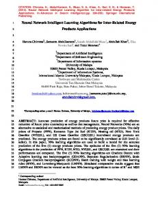
Fig.(3) Linear interpolation.

x

Since we want to find the velocity at t = 16 , and we are using a first order polynomial, we need to choose the two data points that are closest to t = 16 that also bracket t = 16 to evaluate it. The two points are t 0 = 15 and

t1 = 20 . Then

t 0 = 15, v(t 0 ) = 362.78 t1 = 20, v(t1 ) = 517.35 gives 1 t −t j L0 (t ) = ∏ j =0 t 0 − t j j ≠0

t − t1 t 0 − t1 1 t −t j L1 (t ) = ∏ j = 0 t1 − t j

Fig. (2) Graph of velocity vs. time data for the rocket example.

=

Table 1: Velocity as a function of time.

t (s)

v(t ) (m/s)

0

0

10

227.04

15

362.78

20

517.35

22.5

602.97

30

901.67

Determine the value of the velocity at t = 16 seconds using a first order Lagrange polynomial.

  Solution  For first order polynomial interpolation (also called linear interpolation as shown in Fig. (3)), the velocity is given by

j ≠1

t − t0 t1 − t 0 Hence

=

v(t ) =

=

t − t0 t − t1 v(t 0 ) + v(t1 ) t 0 − t1 t1 − t 0

t − 20 t − 15 (362.78) + (517.35), 15 ≤ t ≤ 20 15 − 20 20 − 15

v(16) =

16 − 15 16 − 20 (517.35) (362.78) + 20 − 15 15 − 20 = 0.8(362.78) + 0.2(517.35) = 393.69 m/s

IJCSNS International Journal of Computer Science and Network Security, VOL.11 No.3, March 2011

L0 (t ) = 0.8 and L1 (t ) = 0.2 are like weightages given to the velocities at t = 15 and t = 20 to calculate the velocity at t = 16 . You can see that

4. Back –Propagation Neural Network The back propagation neural is a multilayered, feed forward neural network and is by far the most extensively used. Back Propagation works by approximating the nonlinear relationship between the input and the output by adjusting the weight values internally. A supervised learning algorithm of back propagation is utilized to establish the neural network modeling. A normal backpropagation neural (BPN) model consists of an input layer, one or more hidden layers, and output layer. There are two parameters including learning rate (0 < α