South China Sea Tsunami Workshop 2008
Simulating Tsunami Shallow-Water Equations with Graphics Accelerated Hardware (GPU) and Radial Basis Functions (RBF) J. Schmidt1, C. Piret2, B.J. Kadlec3, D.A. Yuen4*, E. Sevre4, N. Zhang5, Y. Liu4 1
College of Saint Scholastica, Duluth, Minnesota, 55811 USA National Center for Atmospheric Research, Boulder, Colorado, 80305 USA 3 Department of Computer Science, University of Colorado, Boulder, 80309 USA 4 Minnesota Supercomputing Institute, University of Minnesota, Minneapolis, 55455 USA 5 CREST, Medical School, University of Minnesota, Minneapolis, 55455 USA 2
Email:
[email protected] Abstract The rapid growth curves in the speed of GPUs relative to CPUs and its ever-growing popularity have generated a new area in computational technology. We are concerned with modeling tsunami waves, where computational time is of extreme importance. We have employed the NVIDIA board 8600M GT on a MacPro laptop computer to test the efficacy of the GPU on the set of shallow-water equations. We have compared the relative speeds between CPU and GPU on a single processor for two types of spatial discretization based on second-order finite-differences and radial basis functions, which is a more novel method based on a gridless and a multi-scale, adaptive framework. For the NVIDIA 8600M GT we found a speed up by a factor of 8 in favor of GPU for the finite-difference method and a factor of 7 for the RBF scheme. The time steps employed for the RBF method are larger than those used in finite-differences. This ratio of time steps, favoring the RBFs over the finite-difference points, increases with the number of grid points employed. Thus, in modelling tsunami waves over the same physical time transpired, RBF acting in concert with GPU would hold great promise because of the spectacular reduction in the computational time. Key words: Radial Basis Functions, RBF, GPU, tsunami INTRODUCTION Tsunamis commonly strike with little warning. For most people, tsunamis are very much underrated as major hazards [1]. People wrongly believed that they occur infrequently and only along some distant coast. They are usually preceded by earthquakes. Seismic signals usually can give some margin of warning, since the speed of tsunami waves travels at a small fraction of the speed of seismic waves. Still there is not much time, between one hour and a few hours for distant earthquakes and much less, if you are unluckily located in the near field region. Therefore it is important to have codes which are fast to respond to the onset of tsunami waves. It is desirable to have codes which can deliver the output in the course of a few minutes. With the growing popularity of GPU, it is therefore timely to employ this new technology in solving the tsunami wave equations. This may have important consequences in the warning strategy, if an increase in speed of around ten can be obtained on a single CPU. Radial basis functions or RBFs [6] represent a new numerical method, which can also speed up the solution of tsunami wave equations with the traditional finite-difference approach. We will discuss the implementation of both finite-difference and RBFs in the shallow-water approximation for tsunamis [11].
SHALLOW-WATER EQUATIONS We will investigate tsunamis excited by earthquakes. The initial tsunami amplitude waves are very similar to the static, coseismic vertical displacement produced by the earthquake. A practical procedure is to calculate the elastic coseismic vertical displacement field from elastic dislocation theory [10] with a single uniform slip dislocation. We note that because variations in slip are not accounted for, these simple dislocation models may underestimate coseismic vertical displacement that dictates the initial tsunami amplitude. It is only recently [15] that horizontal displacements are deemed to be important in tsunami modelling. After the excitation due to the initial seafloor displacement, the tsunami waves propagate outward from the earthquake source region and follow the inviscid shallow-water wave equation, since the tsunami wavelength is usually much greater than the ocean depths. For water depths greater than about 100 to 400 meters [14, 7], we can approximate the shallow-water wave equations by the set of linear long-wave equations: ∂z / ∂t + ∂M / ∂x + ∂N / ∂y = 0 ∂M / ∂t + g D ∂z / ∂x = 0
(1)
∂N / ∂t + g D ∂z / ∂y = 0 where the first equation represents the conservation of mass and the next two equations govern the conservation of momentum. The instantaneous height of the ocean is given by z(x, y, t), a small perturbative quantity. The horizontal coordinates of the ocean are given by x and y and t is the elapsed time, M and N are the mass fluxes in the horizontal plane along the x and y axes, g is the gravitational acceleration, h(x, y) is the background depth of the ocean, and the total water depth: D(x, y, t) = h(x, y) + z(x, y, t)
(2)
We point out here that the real advantage of the shallow water equation is that z is a small quantity, which allows it to be computed accurately. The three variables of interest in the shallow-water equations are z(x, y, t), the instantaneous height of the seafloor, and the two horizontal velocity components u(x, y, t) and v(x, y, t). We will employ the height z as the principal variable in the visualization. The wave motions will be portrayed by the movements of the crests and troughs in the wave height z, which are advected horizontally by u and v. A rough guide states that one should haves 30 grid points covering the wavelength of a tsunami wave. For a tsunami with a wave period of 5 minutes, this criterion requires a grid size of 100 m and 500 m where the depth of the water exceeds respectively 10 m and 250 m. Accurate depth information is more important than the width of the grid in modelling tsunami behavior close to the coast. The shallow-water equations describing tsunamis are best employed for distances about a few hundred kilometers from the source of earthquake excitation. GRAPHICS PROCESSING UNIT (GPU) A graphics processing unit (GPU) typically is a device that is dedicated to the rendering of 3-D graphics. However, a GPU can also be used to compute complex mathematical operations, thereby lifting the burden off the CPU and allowing it to dedicate its resources to other tasks. When our research group found out the potential speedup of implementing simulations with a GPU, we then decided to investigate whether we could adapt our computational problems to run them on a GPU as well. We looked at modelling tsunamis through two different methods, one was the finite difference method, and the other involved radial basis functions. The GPU used to implement the finite difference method tsunami simulation was an NVIDIA GeForce 8800, while we used an NVIDIA GeForce 8600M GT to implement the radial basis function simulation. These GPUs permitted the simulations to run quicker than running the simulations on the CPU alone. Hence, we wish to run the tsunami simulations on a GPU and determine the speedup from the simulations using just the CPU.
The GPU has multiple types of memory buffers available on it, and they can help to speed up a simulation. Our simulations use texture and linear memory. There are significant advantages to reading from texture memory as compared to global GPU memory, which is necessary to experience the full benefits of the GPU architecture. Textures act as low-latency caches that provide high bandwidth for reading and processing data. Thus, we are able to read data on the GPU very quickly, because it is essentially a memory cache. Textures also provide for linear interpolation of voxels through texture filtering that allows for ease of calculations done at sub-voxel precision. For further technical details, the reader can consult the CUDA Programming Guide [9]. We would also like eventually to carry out visualizations while the simulation is running. This would be accomplished by creating a graphical user interface to show the tsunami propagating through the water as the data is computed. Right now we output a file every sixty time steps to visualize the tsunami. After the simulation has finished running, we take those files and import them into visualization software called Amira [13]. However, the file writing process is quite time consuming because the CPU must write out the file. Therefore, our simulation is constantly copying data to the CPU in order to write the file and then back to the GPU to perform our computations. By eliminating the constant movement between the CPU and the GPU, greater speedup could be attained. Ultimately, we would like to visualize in real time the projected path of the tsunami. In order to program the GPU, we employed the programming language developed by NVIDIA in 2007 called CUDA (Compute Unified Device Architecture). CUDA is a hardware and software architecture designed for issuing and managing general purpose computations on the GPU. This allows the GPU to be used as a data-parallel supercomputer with no need to write functions within the restrictions of a graphics API. CUDA is designed by NVIDIA for their G8x series of graphics cards, which includes the GeForce 8 Series, the Tesla series, and some Quadro cards. Before GPU programming languages became widely accessible, the only way to program a GPU was through assembly language. But assembly language is very difficult to implement; therefore, not many people attempted GPU programming. Recently, GPU programming has become more accessible through the development of a variety of languages. The CUDA programming interface is an extension to the C programming language and therefore provides a relatively easy learning curve for writing programs that will be executed on the device. The resulting program, which we call a kernel, needs to be written as an isolated function that can be executed many times on any block of the data volume. The figure below shows how a CUDA kernel can be written and how it is called from the main program. This example doubles every value stored in the array, using addition. Figure 1 represents the kernel that will be executed inside the GPU. __global__ void addArray (int *a, int size) { int i = blockIdx.x * blockDim.x + threadIdx.x; if (i < size) a[i] = a[i] + a[i]; } Figure 1: A simple example of a CUDA kernel. It displays how arrays can be added together on the GPU. RADIAL BASIS FUNCTIONS (RBF) RBF METHOD Hardy (1971) introduced the RBF methodology in a mapping problem where scattered bivariate data needed to be interpolated to represent topography and produce contours. The common interpolation methods of the time (e.g. Fourier series, polynomials, bivariate splines) were not guaranteed to produce a non-singular system with any set of distinct scattered nodes. His method was innovative in that it represented the interpolant as a linear combination of one basis function (originally the multiquadric function, Figure 2), centered at each node location, making the basis terms dependent on the nodes to be interpolated. All radial functions have the particular property to only depend on the Euclidean distance from their center, making
them radially symmetric. The name of the method was therefore generalized to the Radial Basis Functions (RBF) method. It is not until the 1990s that RBFs were employed to solve PDEs [3]. It offers tremendous prospects for tsunami modelling.
Figure 2: The RBF method consists in centering a radial function at each node location and requiring that the interpolant assume value of the function at the node. RBF REPRESENTATION Given the data values fi at the scattered node locations xi, i =1, 2, . . . , n in d dimensions, a radial basis function interpolant takes the form n
s ( x) =
∑ λ φ( x − x ) i
i
(3)
i =1
where || · || denotes the Euclidean L2-norm. The expansion coefficients λi are obtained by solving a linear system Aλ = f, imposing the interpolation conditions s(xi) = fi. There are two kinds of radial functions, the piecewise smooth and the infinitely smooth radial functions. The piecewise smooth radial functions have a jump in one of their derivatives, which limits them to yielding only an algebraic accuracy. The infinitely smooth radial functions, on the other hand, offer spectral accuracy. They have a shape parameter, ε, which controls how steep they are. The closer this parameter is to 0, the flatter the radial function becomes. We now examine in their simplest form, the equations that govern tsunami phenomena. The linearized long wave equations without bottom friction in two dimensional propagation take the form of the coupled system, similar to those given above in (1) and (2). ηt + Mx + Ny = 0
(4)
Mt + D(x, y) ηx = 0
(5)
Nt + D(x, y) ηy = 0
(6)
where η is the water depth, and M and N are the discharge fluxes in the x and y directions, respectively. The function D(x, y) in equations (5) and (6) incorporates the bathymetry. We assume for sake of simplicity periodic boundary conditions.
The most commonly used methods in tsunami modelling are finite difference schemes. The goal of this section is the show, by comparing RBFs with such a scheme, that radial basis functions, although more computationally expensive, have the potential to outperform the commonly used methods. The staggered leapfrog method (SL) is particularly well-suited for this type of PDE (equations (4), (5) and (6)) and a simple geometry will allow for the grid staggering. It is a second order method both in space and in time. For the sake of simplicity, instead of computing the analytic solution to the system, we choose a convenient solution to equation (4) (η(x, y) = e-t/10sin(x)(-sin(y) + cos(y)), M(x, y) = 1/10e-t/10cos(x)sin(y) and N(x, y) = 1/10e-t/10sin(x)sin(y)), which creates forcing terms in equations (5) and (6). This new system is the one that we solve numerically using the RBF and the staggered leapfrog schemes. The domain is a square equispaced grid, with N total nodes (N1/2 x N1/2 regular grid). Table (1) shows the relative max-norm error computed after a fixed time of t = 5, along with the minimum amount of grid points and the maximum possible time-step to reach it. We see that for a similar error, the method of lines with RBF used in the spatial discretization, and a 4th order Runge-Kutta scheme used in advancing the large set of ordinary differential equations associated with each grid point in time [2, 12], (this is what we refer to when we mention the “RBF method” in this section) allows for much larger time-steps and requires a much sparser grid than the leapfrog method. In realistic cases, using a method such as the staggered leapfrog method, we are expecting N to range from 6502 to 12002. The asymptotic behaviors of the different curves allow to determine that, to obtain an equivalent error with the RBF method, we will only need N to be from 392 to 432 and the time steps will be from 24 to 41 times larger than the steps required when using the staggered leapfrog scheme. This observation is consistent with Flyer and Wright’s findings in [5] and in [4] that although the RBF method has a higher complexity than most commonly used spectral methods, RBFs require a much lower resolution and a surprisingly larger time step than these methods. Overall, RBFs have therefore the potential to outperform these methods both in their complexity and in their accuracy. In addition, RBFs have the clear advantage of not being tied to any grid or coordinate system, making them suitable for difficult geometries. All this added to the code’s undeniable simplicity makes the RBF method an excellent alternative to the commonly used methods, in tsunami modelling. Table 1: Comparison between RBF and the staggered leapfrog (SL) methods. We compare the smallest resolution and the largest time step allowed by each method to yield a similar error. Method RBF SL
Rel. l∞ Error 9.34e-3 1.08e-2
N 192 202
Δt 1.00 0.35
Rel. l∞ Error 8.94e-4 1.04e-3
N 262 652
Δt 0.55 0.11
Rel. l∞ Error 1.01e-4 1.05e-4
N 322 1852
Δt 0.38 0.037
In order to run the RBF simulation in conjunction with a GPU, we used software developed by AccelerEyes called Jacket. By using Jacket, we are able to access the GPU without leaving the MATLAB environment. Jacket is an engine that runs CUDA in the background, eliminating the need for the user to know any GPU programming languages. Instead of writing CUDA kernels, one instructs the MATLAB environment when and what should be transferred to the GPU and then when to copy it back to the CPU [8]. Figure 3 shows an example on how to implement MATLAB code on the GPU by using Jacket. A = eye(5); A = gsingle (A); A = A * 5; A = double (A);
% creates a 5x5 identity matrix % casts A from the CPU to the GPU % multiplies matrix A by a scalar on the GPU % casts A from the GPU back to the CPU
Figure 3: Demonstrates how a MATLAB program can take advantage of the GPU by using the software Jacket. Since Jacket wraps the MATLAB language into a form that is compatible with the GPU, the commands that would have otherwise been written in C are eliminated. However, the CUDA drivers and toolkit must be installed on the computer before Jacket can be used. Additionally, once MATLAB has
opened, a path needs to be added to the Jacket directory so that MATLAB knows where it can access the files that would allow it to cast the data onto the GPU. Moreover, we are visualizing images on the GPU through MATLAB because, thus far, Jacket only supports OpenGL in Linux. Soon one can use Jacket with support of OpenGL. We shall then be able to visualize the RBF within the native MATLAB environment on any computer that supports CUDA, thereby eliminating the step of writing data back to the CPU. Thus, by using RBFs to model tsunamis in conjunction in the GPU would enable us to visualize the tsunami faster than it is propagating through the water, allowing a tsunami warning to be issued swiftly. Figure 4 demonstrates how our simulation in MATLAB currently works.
Jacket MATLAB
Computations performed on the GPU
Jacket
Write data to files (CPU)
Visualize using Amira
Figure 4: The configuration of the current MATLAB simulation. After implementing both the finite difference method and the radial basis function shallow-water simulations on the GPU using CUDA, we received significant speedup in the simulation's run times. The finite difference method simulation was run upon an NVIDIA 8800 GPU. This simulation has a two dimensional grid size of 601 by 601 and contains 21,600 time steps where each time step represents one second. Originally, the simulation was run upon an Opteron-based system in its original form of FORTRAN 77 and it took over four hours to complete its run. However, running the same simulation in conjunction with the GPU took approximately half an hour. Thus, the simulation was about eight times faster than using the CPU alone. However, even with the GPU, we are still outputting a file every sixty time steps so that we can carry out the visualization. If we could eliminate writing data to a file, but rather produce images in real time, the speedup would be increased because of the time it takes to copy the data back to the CPU. Figure 5 shows a visualization of the data with the Amira visualization package [13]. If we could eliminate writing data to a file, but rather produce images in real time, the speedup could be increased since it takes a considerable amount of time to copy data back to the CPU [16]. Therefore, implementing a visualization interface using OpenGL would allow us to visualize the data as it is being created.
Figure 5: Linear tsunami waves calculated on a GPU as visualized by Amira package. The first image (A), shows the tsunami early in its propagation, while the second one, (B), illustrates the tsunami later in the simulation. Visually, there is no difference in running the simulation on the GPU than the CPU. We have also implemented the radial basis function simulation on an NVIDIA 8600 GPU using the software Jacket. Comparing the simulation that ran strictly on the CPU of a MacBook Pro to the simulation
implemented on its GPU, the speedup we received was about seven times faster. This simulation contained four hundred time steps and a grid size of 30 by 30. Overall, we found that running a RBF simulation in conjunction with the GPU would produce the speediest results, thereby allowing the shortest time in issuing a tsunami warning. Our results show that GPU combined with RBFs can be a very powerful combination in solving linear tsunami wave equations in the shallow-water approximation. These calculations can be carried out on laptops without going over to workstations or cluster of computers. Thus they are very useful for remote areas and developing countries in tsunami-prone places around the circum-Pacific belt. Acknowledgements
We thank Gordon Erlebacher, Mark Wang, Natasha Flyer, Grady Wright, Tatsuhiko Saito, and Takahashi Furumura for helpful discussions. D. A. Yuen also expresses support from Earthquake Research Institute, University of Tokyo. This research has been supported by NSF grant to the Vlab at the Univ. of Minnesota. REFERENCES 1. Bryant, E., Tsunami: The Underrated Hazard, 330 pp. second edition, Springer Verlag, Heidelberg,
2008. 2. Dahlquist, G. and A. Bjoerck, Numerical Methods in Scientific Computing, Vol. 1., SIAM,
Philadelphia, 2008. 3. Fasshauer, G. E., Meshfree Approximation Methods with Matlab, World Scientific Publishing,
Singapore, 2007. 4. Flyer, N., and Wright, G., A radial basis function shallow water model, submitted J. Comp. Phys.,
2008. 5. Flyer, N. and G. Wright, Transport schemes on a sphere with radial basis functions, J. Comp. Physics,
2007, 226: 1059-1084. 6. Fornberg, B. and Piret, C., A stable algorithm for at radial basis functions on a sphere, SIAM J. Sci.
Comput., 2007, 200: 178-192. 7. Liu, Y., Santos, A., Wang, S.M., Shi, Y., Liu, H. and D.A. Yuen, Tsunami hazards along the Chinese
coast from potential earthquakes in South China Sea, Phys. Earth Planet. Inter., 2007, 163: 233-244. 8. Melonakos, J., Parallel computing on a personal computer, Biomedical Computation Review, 2008, 4,
29. 9. NVIDIA CUDA Compute Unified Device Architecture, Programming Guide, Version Beta 2.0, June 7,
2008. 10. Okada, Y., Surface deformation due to shear and tensile faults in a half-space, Bull. Seismological Soc.
America, 1985, 75: 1135-1154. 11. Satake, K., Tsunamis, in W.H. K. Lee, H. Kanamori, P. C. Jennings, and C. Kisslinger (eds.)
International Handbook of Earthquake and Engineering Seismology, 2002, 81A: 437-451. 12. Schiesser, W. E., The Numerical Method of Lines, Academic Press, San Diego, 1991. 13. Sevre, E., Yuen, D. and Y. Liu, Visualization of tsunami waves with Amira package, Visual
Geosciences, 2008, 13: 85-96. 14. Shuto, N., Goto, C. and F. Imamura, Numerical simulations as a means of warning for near-field
tsunamis, Proceedings of the Second UJNR Tsunami Workshop, Honolulu, Hawaii, November 5-6, 1990, National Geophysical Data Center, Boulder, 1991, pp. 133-153.
15. Song, Y.T., Fu, L.L., Zlotnicki, V., Ji, C., Hjorleifsdottir, V., Shum, C.K. and Y. Yi, The role of
horizontal impulses of the faulting continental slope in generating the 26 December 2004 tsunami, Ocean Modelling, 2008, 20: 362-379. 16. Weiskopf, D., GPU based interactive visualization techniques, 312 pp. first edition, Springer Verlag,
New York, 2006.