APCOM’07 in conjunction with EPMESC XI, December 3-6, 2007, Kyoto, JAPAN
A System-Model-Based Design Environment for 3D Simulation and Animation of Micro-Electro-Mechanical Systems (MEMS) Gunar Lorenz1 and Mattan Kamon2 1
Coventor SARL, av. du Quebec, ZI de Courtaboeuf, 91140Villebon sur Yvette, France Coventor Inc., 625 Mount Auburn Street, Cambridge, MA 02138, USA e-mail:
[email protected],
[email protected], 2
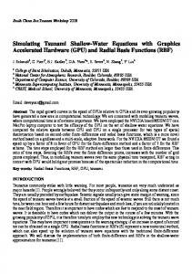
Abstract We will describe recent advances in CoventorWare ARCHITECTTM, a comprehensive MEMS design and simulation environment. In ARCHITECT, MEMS designers work in a schematic driven environment using symbols that represent individual components or elements of components. These symbols are connected and parameterized in the schematic to represent a three dimensional MEMS device. The schematic symbols and the mathematical models that they represent enable exploration of the parametric design space in seconds or minutes with accuracy that rivals finite element analysis. Previously, schematic-driven MEMS design environments, while extremely fast, had a fundamental obstacle to widespread acceptance: they lacked a three-dimensional view. The three-dimensional geometry was represented abstractly with symbols and parameters, and the simulation results were two-dimensional plots of individual degrees of freedom of the structure. In this article we describe a new companion 3D visualization tool, Scene3D that, when combined with fast simulation speed of ARCHITECT, provides unprecedented insight into the complex dynamic behavior of MEMS devices. Scene3D is useful both during schematic creation and for quickly interpreting simulation results. From a user perspective, “one button click” creates 3D views of any ARCHITECT schematic and enables designers to visualize simulation results in colorful three-dimensional animations that make it much easier to understand the dynamic behavior of a MEMS device. Key words: MEMS, System Modeling, Animation, MEMS-IC Co-simulation INTRODUCTION Mathematical modeling, based on analytically derived formulas, has always been a part of MEMS design. Over the years, mathematicians and engineers have built up a vast framework for engineering mathematics and applied it to MEMS design. Coventor has encapsulated much of this knowledge into a commercial product called CoventorWare ARCHITECTTM [1]. ARCHITECT is built around component libraries that embody many years of development effort and Coventor’s experience in working closely with leading MEMS suppliers [2][3]. ARCHITECT enables MEMS designs that are so complex, that conventional finite element modeling is not feasible [4]. In ARCHITECT, MEMS designers work in a schematic driven environment using symbols that represent individual components or elements of components as seen in Figure 1. Typically, these component models are parameterized, i.e. they take as input a few parameters such as width and length, so that the same mathematical model can be used for different versions of the same type of component, see Figure 2. ARCHITECT includes parametric component libraries for various MEMS applications, allowing users to study how the individual components behave when subjected to electrical and mechanical stimuli, and stimuli from other physical domains. The complex mathematical description used with high-level models leads to a small number of degrees of freedom, making it practical to investigate MEMS devices in a much more spontaneous manner than with traditional finite element techniques. Complete systems, including peripheral subsystems (for example, sensing and driving circuits) can be built in a common design environment and simulated in a matter of seconds or minutes.
ARCHITECT’s state-of-the-art MEMS system models offer such a rich geometric parameterization that they can be used for rapid virtual prototyping with a level of accuracy that rivals standard finite element/boundary element approaches.
Figure 1: Schematic model of a MEMS gyroscope with illustrations of the physical geometry represented by some of the schematic symbols
Figure 2: Model parameters of an electrostatic comb struture
MEMS devices are surrounded by electronic circuitry needed for feedback loops and signal processing. Using a schematic modeling environment for MEMS simulations is a straightforward choice considering that device and integrated circuit (IC) designers have to work hand-in-hand to design and optimize the whole system. Creating a library of mechanical, electrostatic, piezo-electric, magnetic and optical models that are compatible with existing electronic component libraries has the clear advantage of simulating a complete multi-physics system in a single simulation environment. Unfortunately, there are a number of drawbacks to applying an IC-oriented schematic environment to MEMS design. Schematics representing MEMS are abstract representations of 3D geometry rather than direct geometric topology as is represented by the solid model and mesh in a finite element environment. In a schematic environment, as shown in Figures 1 and 2, the geometry, position and orientation of each modeled substructure are defined by the parameters of the corresponding schematic symbol, not by an external graphical 3D solid modeling tool. Minor parameter changes can result in substantially different device geometry. While conventional IC design tools allow the user to extract a two-dimensional layout from a schematic, they do not include the 3D visualization capability needed to understand and verify the parameter settings and symbol connectivity of non-electrical structures like MEMS. Additionally, and maybe even more importantly, working efficiently with MEMS models requires a 3D environment for visualizing the change in shape, orientation and position of the modeled structures as predicted by simulating the schematic. Unfortunately, conventional IC system modeling environments make it difficult to interpret simulation results that include non-electrical components. In conventional IC schematics, electrical “wires” connect the schematic symbols. The results of schematic circuit simulations, such as voltage and current changes over time or frequency on individual wires, can be displayed graphically in 2D “X-Y plots”. Two-dimensional X-Y plots are generally sufficient for understanding purely electrical circuits. MEMS simulations, however, involve spatial displacements and/or rotations of the mechanical substructures. The symbols that represent the MEMS components or substructures are linked by mechanical “wires” that are associated with mechanical degrees of freedom, such as spatial displacements, rotations, forces, or torques. Similar to simulations of electrical circuits, these non-electrical quantities from MEMS simulations can be displayed in X-Y plots. As an example Figure 3 shows the schematic of a double mass gyroscope with two large, perforated plates that are driven sinusoidally in the x direction and out of phase from one another by the comb actuators on the ends. The device operates by exploiting the fact that angular motion generates a Coriolis force that moves the plates up and down and out of phase with one another allowing differential sensing through the capacitance to electrodes underneath the plates. To understand a simulation result, one needs to understand the motion of both the plates, their relation to each other as well as their suspension beams. However, with X-Y plots, the designer is limited to seeing the motion of a single degree of freedom at a time, such as the motion of a one rigid plate along the X-axis as a function of time as shown in Figure 3. These X-Y plots are insufficient considering that the complete interpretation of just a single plate requires six X-Y plots (three for the translational and three for the rotation degrees of freedom). If X-Y plots generate some inconvenience for the interpretation of a single plate they are extremely cumbersome when in comes to interpreting the motion and deformation of the whole structure of Figure 3, especially considering that it features a total of 108 mechanical degrees for freedom. In this article we describe a new companion 3D visualization tool, Scene3D [5][6], that overcomes the obstacles of designing MEMS in an IC-oriented environment. The following two sections describe the generation of geometric representations of schematic symbols and mechanical “wires”. Afterwards and perhaps most importantly, we describe how schematic simulation results can be turned into colorful, three-dimensional animations.
Figure 3: Transient simulation of the x-direction motion of a single plate of the gyroscope 3D VIEW GENERATION Scene3D enables users to generate a three-dimensional view of a MEMS device model captured in an ARCHITECT schematic with a single button click. The 3D view generation starts by analyzing the mechanical components in the given MEMS schematic. Each MEMS component in the ARCHITECT model library is associated with a corresponding 3D view generator in Scene3D, see Figure 4. The 3D view generators create a 3D ACIS® entity based on the parameters of the corresponding schematic model. The 3D views of each model component collectively compose the overall 3D model of the MEMS device. ACIS®, a product of Spatial Technologies (www.spatial.com/products/acis.html), has an object-oriented C++ architecture that enables robust, 3D modeling functionality. Since ACIS geometry is supported by most state-of-art CAD tool providers, models created with ARCHITECT Scene3DTM can be easily exported to existing CAD and finite element tools via the widely-used 3D .sat file format. The actual visualization of the ACIS model in the Scene3D canvas is done by the HOOPS 3D Application framework (HOOPS/3dAF). HOOPS/3dAF, a product of Tech Soft 3D (www.techsoft3d.com), provides C++ bindings to tessellate (generate a skin of triangles) each ACIS model and visualize the model on the 3D graphics canvas. HOOPS/3dAF also provides standard features like rotating, zooming, scaling, and suppressing the display of individual components.
Figure 4: 3D view of a MEMS schematic model of a double mass gyroscope generated with Scene3D In Scene3D, the canvas with the 3D view of the MEMS device is accompanied by a symbolic view containing a hierarchical list of schematic component names. The symbolic/tree view allows crossreferencing of the symbolic view and the 3D graphical view as shown in Figure 4. Cross-referencing between the different views allows the user to correlate 3D model entities with the corresponding component in the schematic view. Parameter errors can be quickly identified and corrected in the schematic editor. MECHANICAL WIRE REPRESENTATION IN 3D The wires linking electrical symbols in an electrical schematic have a direct analogy in the physical world: they represent a physical wire that keeps its two ends constrained to the same voltage. The wires linking the mechanical components in a MEMS schematic lack a direct physical analogy, however the function is similar: they keep their two ends constrained to move together. In ARCHITECT schematics, mechanical wires are a bundle of 6 individual wires containing three translational and three rotational wires. The values of the six mechanical sub wires define the motion and the rotation of a mechanical point in space. This point, referred to as “knot”, can be seen as the physical connection point between two or more mechanical elements, see Figure 5.
Figure 5: Mechanical wire representation in Scene3D A knot is similar to the concept of a finite element node whose six degrees of freedom are shared between all the finite elements connected to that node and thus constrain the elements to move together. Beam elements in ARCHITECT have one knot for each end just like finite element beams have two nodes. The knot extends the concept of a finite element node by allowing the physical point on the element to be different from the location of the knot. Knots are a powerful concept for linking rigid and flexible elements in the same schematic. Rigid schematic components like combs and rigid plates are connected to only one knot. The six degrees of freedom of a knot, plus the knowledge of its initial position, are sufficient to define a rigid component’s position and orientation in space. In Figure 5, the location of the highlighted knot is in the center of a large rigid plate and the yellow lines, called “knot connections”, point to the physical entities that are tied to the same knot. The knot corresponding to the highlighted mechanical wire in the ARCHITECT schematic ties a rigid plate, an electrode underneath, two comb structures as well as the beam end faces of the four suspensions together. Scene3D provides a special knot viewing mode that highlights all initial knot positions and knot connections inside the transparent components of the MEMS device. Furthermore, a special knot tree view allows the user to correlate selected knots on canvas with the corresponding mechanical wire names in the schematic model as shown on the left of the window in Figure 5. RESULT VISUALIZATION One of the most powerful features of Scene3D is its ability to visualize schematic simulation results in a 3D environment. Circuit simulation involving mechanical components can be seen as a calculation of knot motions and rotations under given mechanical, electrical, thermal, magnetic or any other physical stimuli. Depending on the chosen type of analysis (e.g. steady state (DC), harmonic (AC) or transient analysis) the
knot motions are calculated as a function of time, frequency and/or system model parameters, respectively. The knot motions however only tell part of the story. For instance, the translations and rotations of the two knots at the ends of a beam component indicate only the motion of the beams ends, yet determine the deformation of the entire beam through its shape function. Visualizing the entire simulation result thus involves mapping the knot motions to the translation, rotation, and deformation of all the mechanical components of the schematic. The results of circuit simulations are stored and updated in result files that contain the translations and rotations of every knot. Depending on the type of analysis, the result file may include just one set of values, or a list of values, for each knot. Lists of values may include the knot displacement and rotation data for each time step (transient analysis), each frequency (AC analysis) or each parameter increment (DC transfer or vary analysis). In Scene3D users can load simulation result files and visualize the corresponding model deformation. The animations are created by executing the 3D generator associated with each component in the list. The 3D view generators make use of not only the component’s parameter values, but also use the simulated knot position and orientation as input to the component’s shape function, to create a graphical 3D view of the component. The resulting graphical views of the components may show displacements and deformations if the knot position and orientation differ from their nominal values as shown in the close up view of Figure 6. Simulation results that contain lists of values are passed to the generators sequentially, one per time step, frequency point, etc. The continuous update of the individual 3D views by the corresponding 3D generators can be seen as an animated motion of the whole mechanical structure.
Figure 6: Close look-up at a structure deformed by AC simulation results
Note that in a finite element environment, simulating the 1000 frequency points of the coupled electromechanical harmonic analysis in Figure 7 could take hours. In addition, storing all the harmonic data would take up gigabytes of storage space. Loading and scanning through the frequency points alone would require minutes. With ARCHITECT and Scene3D, simulating 1000 frequency points takes seconds, the storage needed is minimal, and each frequency point can be visualized in a fraction of a second.
Figure 7: Result visualization of a harmonic simulation CONCLUSIONS In this article we presented Scene3D, the latest addition to our schematic-based MEMS design environment, CoventorWare ARCHITECTTM. ARCHITECT and Scene3D form a comprehensive virtual prototyping tool for MEMS that not only rivals standard finite element/boundary element approaches in accuracy, but also in user friendliness. Scene3D overcomes the abstract nature of IC schematic environments by providing state-of-art 3D model and result visualization. REFERENCES [1] D. Teegarden, G. Lorenz, R. Neul, How to model and simulate microgyroscope systems. IEEE Spectrum „Art & Technology“, July 1998 Vol. 35 No. 7, pp 66-75 [2] G. Lorenz and J. Repke, Design Tools for MEMS, Sensors Applications, Volume 4, Sensors in Automotive Technology, Jossey-Bass Publishers (A Wiley Company), ISBN: 3527295534, p. 58-72 [3] C. Kennedy, M. Bellrichard, M. Weber, High Angular Rate and High q Effects in the MEMS Gyro, Sensor Magazin, November 2004
[4] G. Lorenz, R. Neul, Network-Type Modeling of Micromachined Sensor Systems. Proc. Int. Conf. on Modeling and Simulation of Microsystems, Semiconductors, Sensors and Actuators, MSM98, Santa Clara, April 1998, pp. 233-238. [5] G. Lorenz, 2005, A system and method for three-dimensional visualization and postprocessing of a system model, U.S. Patent 7,263,674 [6] M. Kamon, G. Lorenz, S. Breit, System and method for process-flexible MEMS design and simulation, U.S. Patent 7,272,801