Oct 13, 2005 - on local linear fits over asymmetric intervals of the form [x0 − (1 − λ)h, x0 + (1 + ... indicates the strength of the dependence between Y and X near each X = x. ... obtained as the slope of the least squares estimate of β(x0) computed for data in the ... shrink to a point as n goes to infinity, the asymptotic power is ...
Powerful Choices: Tuning Parameter Selection Based on Power Kjell A. Doksum∗ and Chad M. Schafer† University of Wisconsin, Madison and Carnegie Mellon University
October 13, 2005
Abstract We consider procedures which select the bandwidth in local linear regression by maximizing the limiting power for local Pitman alternatives to the hypothesis that µ(x) ≡ E(Y | X = x) is constant. The focus is on achieving high power near a covariate value x0 and we consider tests based on data with X restricted to an interval containing x0 with bandwidth h. The power optimal bandwidth is shown to tend to zero as sample size goes to infinity if and only if the sequence of Pitman alternatives is such that the length of the interval centered at x 0 on which µ(x) = µn (x) is nonconstant converges to zero as n → ∞. We show that tests which are based on local linear fits over asymmetric intervals of the form [x0 − (1 − λ)h, x0 + (1 + λ)h], where −1 ≤ λ ≤ 1, rather than the symmetric intervals [x0 −h, x0 +h] will give better asymptotic power. A simple procedure for selecting h and λ consists of using order statistics intervals containing x0 . Examples illustrate that the effect of these choices are not trivial: Power optimal bandwidth can give much higher power than bandwidth chosen to minimize mean squared error. Because we focus on power, rather than plotting estimates of µ(x) we plot a correlation curve ρb(x) which
indicates the strength of the dependence between Y and X near each X = x. Extensions to more general hypotheses are discussed.
1
Introduction. Local Testing and Asymptotic Power.
We consider (X1 , Y1 ), (X2 , Y2 ), . . . , (Xn , Yn ) i.i.d. as (X, Y ) ∼ P and write Y = µ(X) + � where µ(X) ≡ E(Y | X) and β(x) ≡ dµ(x)/dx are assumed to exist, and � ≡ Y − µ(X). We are interested in a particular covariate value x0 and ask if there is a relationship between the response Y and the covariate X for X in some neighborhood of x 0 . More formally, we test the hypothesis H that ∗ †
Supported in part by NSF grants DMS-9971309 and DMS-0505651. Supported in part by NSF grant DMS-9971301.
1
β(x) = 0 for all x against the alternative K that β(x) 6= 0 for x in some neighborhood of x 0 . Our focus is on achieving high power for a covariate value x 0 for a unit (patient, component, DNA sequence, etc.) of interest. We want to know if a perturbation of x will affect the mean response for units with covariate values near x 0 . Our test statistic is the t-statistic t h (x0 ) based on the locally linear estimate βbh (x0 ) of β(x0 )
obtained as the slope of the least squares estimate of β(x 0 ) computed for data in the local data set Dh (x0 ) ≡ {(xi , yi ) : xi ∈ Nh (x0 )} , with Nh (x0 ) ≡ [x0 − h, x0 + h] . The bandwidth h serves as a lense with different lenses providing insights into the relationship between Y and X (Chaudhuri and Marron (1999, 2000) did “estimation” lenses). The h that
maximizes the power over Nh (x0 ) provides a customized lense for a unit with covariate value x 0 . We discuss global alternatives where supx |β(x)| > 0 in Remark 2.3. The many available tests for this alternative will have increased power if they are based on variable bandwidths. We will next show that the power of the test is very sensitive to the choice of h and that this choice at first appears to be inversely related to the usual choice of h based on mean squared error (MSE). In fact, for any alternative with β(x) nonzero on an interval centered at x 0 that does not shrink to a point as n goes to infinity, the asymptotic power is maximized by selecting an h = h n that does not converge to zero as n → ∞.
Because βbh (x0 ) is asymptotically normal, the asymptotic power of the test based on it for local
Pitman alternatives will be determined by its efficacy (EFF) for one-sided alternatives β(x) > 0 and by its absolute efficacy for two-sided alternatives β(x) 6= 0 (Kendall and Stuart (1961), Section 25.5, Lehmann (1999)): i�1/2 i�� h � h � . VarH βbh (x0 ) EFFh ≡ EFF βbh (x0 ) = EK βbh (x0 )
Consider the alternative µ(x) = α + γ r(x) for a differentiable function r(·). We know (e.g. Fan and Gijbels (1996), pg. 62) that for h → 0, conditionally on X = (X 1 , X2 , . . . , Xn ), i h � EK βbh (x0 ) | X = γr 0(x0 ) + c1 h2 + oP h2 and i h � VarH βbh (x0 ) | X = c2 n−1 h−3 + oP n−1 h−3
for appropriate constants c1 and c2 . These expressions yield an approximate efficacy of order n1/2 h3/2 which is maximized by h not tending to zero (where the expressions are not valid). This
2
shows that h tending to zero does not yield optimal power and that maximizing power is typically very different from minimizing some variant of mean squared error: for example, h i MSE(h) ≡ E (b µh (X) − µ(X))2 1{X ∈ (x0 − h, x0 + h)} , where µ bh (·) is the local linear estimate of µ(·). This subject has been discussed for global alternatives
by many authors, sometimes with the opposite conclusion. For a discussion, see e.g. Hart (1997),
Zhang (2003b), Zhang (2003a), and Stute and Zhu (2005). In the next section we look more closely at the optimal h and find that for certain least favorable distributions, the optimal h does indeed tend to zero. Remark 1.1: Why the t-test? (a) The t-test is asymptotically most powerful in the class of tests using data from D h (x0 ) for a class of perturbed normal linear models defined for x i ∈ Nh (x0 ) by Yi = γ (xi − x0 ) + γ 2 r(xi ) + �, P where (xi − x0 ) = 0. Here, � has the distribution Φ(t/σ 0 ) where γ = γn = O(n−1/2 ) is a Pitman alternative, h is fixed, and r(·) is a general function satisfying regularity conditions. To establish
the asymptotic power optimality, suppose all parameters are known except γ and consider the Rao score test for testing H : γ = 0 versus K : γ > 0. It is easy to see that this statistic is equivalent to
P
(xi − x0 )Yi whose asymptotic power is
the same as that of the t-test. It is known (e.g. Bickel and Doksum (2001), Section 5.4.4) that the score test is asymptotically most powerful level α. In the presence of nuisance parameters, a modified Rao score test retains many of its power properties, see Neyman (1959) and Bickel et al. (2006). The idea of asymptotic optimality for perturbed models is from Bell and Doksum (1966). The asymptotic power optimality of the t-test is in agreement with the result that when bias does not matter, the uniform kernel is optimal (e.g. Gasser et al. (1985) and Fan and Gijbels (1996)). But see Blyth (1993), who shows that for certain models, a kernel asymptotically equivalent to the derivative of the Epanechnikov kernel maximizes the power asymptotically. While for alternatives of this type the use of a test based on the t-test is asymptotically most powerful, there undoubtedly exist other situations in which a test based on an appropriate nonparametric estimate of µ(·) gives better power. We will explore this issue in future work. (b) The t-test is the natural model selector for choosing between the models µ(x) = β 0 + � and µ(x) = β0 + β1 x + �0 in the sense that to minimize mean squared prediction error, we select the √ former model if the absolute value of the usual t-statistic is less than 2 (see e.g. Linhart and 3
Zucchini (1986)). This is easily seen to be equivalent to minimizing the mean squared estimation error. It also is the rule of choice if we apply the methods of Claeskens and Hjorth (2003) who choose the model that minimizes the asymptotic mean squared estimation error for Pitman sequences of alternatives. Remark 1.2: For a given test statistic T , the numerator of the efficacy is usually (e.g. Lehmann (1999), pg. 172, and Kendall and Stuart (1961)) defined in terms of the derivative of E θ (T ) evaluated at the hypothesized parameter value θ 0 . We consider the “pre-derivative” because we want to investigate how h influences efficacy. Remark 1.3: Hajek (1962), Behnen and Hu¯skov´a (1984), Behnen and Neuhaus (1989), Sen (1996), among others, proposed and analyzed procedures for selecting the asymptotically optimal linear rank test by maximizing the estimated efficacy. Remark 1.4: The approach of selecting bandwidth to maximize efficacy can also be used to test a parametric model of the form E(Y |X = x) = g(x; β) against a nonparametric model. Simply begin by subtracting off from Y the appropriate model fit under the (null hypothesis) parametric model. See Remark 2.9.
2
Maximizing Asymptotic Power
We start with fixed h > 0. Then the limiting power for the two-sided alternative is a one-to-one function of the absolute value of � � τh (x0 ) ≡ lim n−1/2 EFF βbh (x0 ) . n→∞
Thus the maximizer of the asymptotic power is h 0 ≡ arg maxh |τh (x0 )|. Our estimate of h0 is the maximizer of the absolute t-statistic, b h ≡ arg maxh |th (x0 )| or its equivalents given in Remark 2.1.
To investigate the limit of the t-statistic, t h (x0 ), for the data Dh (x0 ) we write it as signal/noise where
� d h (X) and d h (X, Y ) Var signal ≡ βbh (x0 ) = Cov � � � � 2 2 b d h (X) . b d nh Var noise ≡ Var βh (x0 ) = Eh �h
d h (X) and Cov d h (X, Y ) denote the sample variance and covariance for the data D h (x0 ), Here Var � n X � 2 b nh ≡ 1{xi ∈ Nh (x0 )} and Eh �h = RSSh (nh − 2) , i=1
4
where RSSh is the residual sum of squares on Dh (x0 ).
P
(yi − µ bL,h (xi ))2 for the linear fit µ bL,h (xi ) to yi based
For fixed h, as n → ∞, P βbh (x0 ) −→ βh (x0 ) ≡ Covh (X, Y ) /Varh (X) , P
(nh /n) −→ Ph (x0 ) ≡ P (X ∈ Nh (x0 )) , and � P � b h �2 −→ E Eh �2L,h ≡ Eh [Y − µL,h (X)]2 , h
where Eh , Varh , and Covh denote expected value, variance, and covariance conditional on X ∈
Nh (x0 ), and where µL,h (x) = αh + βh X with αh and βh the minimizers of Eh [Y − (α + βX)]2 . It follows that as n → ∞, n
−1/2
P
th (x0 ) −→
τh∗ (x0 )
�
� � 1/2 ≡ βh (x0 ) {Ph (x0 ) Varh (X)} Eh �2L,h � � � ��1/2 Eh �2L,h = SDH (Y ) τh (x0 ) . 1/2
(1)
For sequences of Pitman alternatives where µ(x) = µ n (x) converges to a constant for all x as n → ∞, we assume that as n → ∞ � Eh �2L,h → σ 2 ≡ VarH (Y ) .
In this case, τh∗ (x0 ) = τ (x0 ). It is clear that τh∗ (x0 ) → 0 as h → 0 because both Ph (x0 ) and Varh (X) tend to zero while Eh (�2L,h ) does not tend to zero except in the trivial case Y = µ L,h (x) for x ∈ Nh (x0 ). On the other hand, if the density of X has support [a, b] and x 0 ∈ [a, b], then for h0 ≡ max{x0 − a, b − x0 }, lim τh∗ (x0 ) h → h0
�
= βL Var(X)
�
E
�2L
�
�1/2
,
where �L = Y − (αL + βL X) with αL and βL the minimizers of E[Y − (α + βX)]2 , that is, βL = Cov(X, Y )/Var(X), αL = E(Y ) − βL E(X). Thus, when X has finite support [a, b] and x0 ∈ [a, b], the maximum of τh∗ (x0 ) over h ∈ [0, h0 ] exists and it is greater than zero. A similar argument shows that h = 0 does not maximize τ h∗ (x0 ) when X has infinite support. Remark 2.1: Instead of the t-statistic t h (x0 ), we could use the efficacy estimate � � d βbh (x0 ) = rh (x0 ) , EFF 5
where rh (x0 ) is the sample correlation for data from D h (x0 ). The formula � � 2 2 th (x0 ) = (n − 2) rh (x0 ) 1 − rh2 (x0 ) ,
where the right hand side is increasing in |r h (x0 )|, establishes the finite sample equivalence of |th (x0 )| and |rh (x0 )|. They are also similar to |ρ(x0 )| where ρbh (x0 ) = q
c βbh (x0 ) SD(X)
d d h (Y ) βbh2 (x0 ) Var(X) + Var
is the estimate of the correlation curve ρ(·) discussed by Bjerve and Doksum (1993), Doksum et al. (1994), and Doksum and Froda (2000). Here ρbh (x) is a standardized version of rh (x0 ) which is calibrated to converge to the correlation coefficient ρ in bivariate normal models.
2.1
Optimal Bandwidth for Vertical Pitman Sequences
√ If we consider Pitman alternatives of the form Y = α + γr(X) + � where γ = γ n = c/ n, c 6= 0, and |r 0 (x)| > 0 in a fixed interval containing x 0 , then
h i n−1/2 EFF βbh (x0 ) → τh (x0 ) ,
where τh (x0 ) is as in Equation (1), and the optimal h will be bounded away from zero as before. Thus, the power optimal bandwidth does not tend to zero for sequences of alternatives where, as n → ∞, kβk∞ → 0 and kβk−∞ 6→ 0 with kβk∞ ≡ supx |β(x)| and kβk−∞ ≡ x+ (β) − x− (β) ≡ sup {x : |β(x)| > 0} − inf {x : |β(x)| > 0} . x
x
We refer to kβk∞ as the “vertical distance” between H and the alternative and kβk −∞ as the “horizontal discrepancy.” Next we consider “horizontal” sequences of alternatives where kβk −∞ → 0 and kβk∞ may or may not tend to zero as n → ∞ and find that now the power optimal bandwidth tends to zero.
2.2
Optimal Bandwidth for Horizontal Pitman Sequences
We now consider Pitman alternatives of the form �
X − x0 Kn : Y = α + γ W θ
�
+ �,
(2)
where X and � are uncorrelated, � has mean zero and variance σ 2 , and W (·) has support [−1, 1]. We assume that X is continuous, in which case µ(·) is the constant α with probability one when 6
θ = 0. Thus the hypothesis holds with probability one when γθ = 0. We consider models where θ = θn → 0 as n → ∞, and γ may or may not depend on θ and n. For these alternatives the neighborhood where |β(x)| > 0 shrinks to achieve a Pitman balanced model where the power converges to a limit between the level α and 1 as n → ∞. Note, however, that the alternative does not depend on h. We are in a situation where “nature” picks the neighborhood size θ, and the statistician picks the bandwidth h. This is in contrast to Blyth (1993) and Ait-Sahalia et al. (2001) who let the alternative depend on h. Note that for h > 0 fixed, γ bounded above, and θ → 0, � � �� X − x0 →0 Covh (X, Y ) = γCov h X, W θ because W ((X − x0 )/θ) tends to zero in probability as θ → 0 and any random variable is uncorrelated with a constant. This heuristic can be verified by the change of variable s = (x − x 0 )/θ, x = x0 + θs. More precisely, Proposition 2.1: Assume that the density f (·) of X has a bounded derivative at x 0 . If h > 0 is fixed, then as γθ → 0 in the Model (2), (a) Covh (X, Y ) = O(γθ); (b) n−1/2 EFF(βbh (x0 )) → 0; P
(c) n−1/2 th (x0 ) −→ 0.
Proof: Since � is assumed uncorrelated with X, Cov h (X, Y ) = Cov h (X, µ(X)) and hence � � �� X − x0 Covh (X, Y ) = γCov h X, W θ �� � � � Z h x − x0 = γ f (x) Ph (x0 ) dx (x − Eh (X)) W θ −h Z 1 γθ (x0 + sθ − Eh (X)) W (s) f (x0 + sθ) ds = Ph (x0 ) −1 � � Z 1 γθ = (x0 − Eh (X)) f (x0 ) W (s) ds + O(θ) . Ph (x0 ) −1
(3)
Then Result (b) follows because �
�
EK βbh (x0 ) → Covh (X, Y )
�
Varh (X)
and the other factors in EFF h are fixed as θ → 0. Similarly (c) follows from Equation (1). � Proposition 2.1 shows that for model (2), fixed h leads to small |EFF h |. Thus we turn to the h → 0 case. If h > θ then observations (X, Y ) with X outside [x 0 − θ, x0 + θ] do not contribute to 7
the estimation of βh (x0 ). Thus choosing a smaller h may be better even though a smaller h leads to a larger variance for βbh (x0 ). This heuristic is made precise in the next result which provides conditions where h = θ is the optimal choice among h satisfying h ≥ θ. Define mj (W ) ≡
Z
1
sj W (s) ds
j = 0, 1, 2.
−1
Theorem 2.1: Assume that the density f (·) of X has a bounded, continuous second derivative at x0 and that f (x0 ) > 0. Then, in model (2), as θ → 0 and h → 0 with h ≥ θ, the following are true. � γθ 1 (a) Covh (X, Y ) = − m0 (W ) f 0 (x0 ) h2 2hf (x0 ) 3 � � + f (x0 ) m1 (W ) θ + f 0 (x0 ) m2 (W ) θ 2 + o h2 + o θ 2 .
(b) If m1 (W ) 6= 0 and m2 (W ) 6= 0, τh,θ (x0 ) ≡ = + =
�
� b lim n EFF βh (x0 ) n→∞ � 1 σ −1 γθh−3/2 [f (x0 )]−1/2 − m0 (W ) f 0 (x0 ) h2 3 � � f (x0 ) m1 (W ) θ + f 0 (x0 ) m2 (W ) θ 2 + o h2 + o θ 2 � � O σ −1 γθ 2 h−3/2 −1/2
(4)
and |τh,θ (x0 )| is maximized subject to h ≥ θ by h = θ. (c) If m1 (W ) = 0,
� � � � lim n−1/2 EFF βbh (x0 ) = O σ −1 γθ 3 h−3/2
n→∞
and |τh,θ (x0 )| is maximized subject to h ≥ θ by h = θ. Proof: Part (a): This is Lemma 4.3, part (e). Part (b): lim n
n→∞
−1/2
EFFh = σ
−1
�
Covh (X, Y ) (Ph (x0 ))
�
Varh (X)
�1/2
.
By Lemma 4.3, part (d), we get Ph (x0 ) /Varh (X) = 6f (x0 ) h−1 + O(1) . Equation (4) follows from this and part (a). Thus we can write h i lim n−1/2 EFFh � σ −1 c1 γθh1/2 + c2 γθ 2 h−3/2 + c3 γθ 3 h−3/2
n→∞
8
(5)
for appropriate constants c1 , c2 , and c3 given in part (b). The square of the expression on the right of Equation (5) is dominated by [σ −1 θ 2 h−3/2 c2 ]2 and maximized for h ≥ θ by h = θ. Part (c): Apply the argument in Part (b). � It remains to investigate the case where h ≤ θ. We next show that the optimal h cannot be such that h/θ → 0. Proposition 2.2: Assume the conditions of Theorem 2.1 and that W 00 (·) exists and is bounded in a neighborhood of zero. Then, as h/θ → 0, o σ −1 γθ 2 h−3/2 � , if W 0 (0) 6= 0 lim n−1/2 EFFh = . n→∞ o σ −1 γθ 3 h−3/2 � , if W 0 (0) = 0 Proof: Set a ≡ h/θ and define
mj,a (W ) ≡
Z
a
sj W (s) ds, j = 0, 1, 2.
−a
Equation (4) in Theorem 2.1, part (b), with m j (W ) replaced by mj,a (W ) is valid. A Taylor expansion gives � � m1,a (W ) = 2W 0 (0) + aW 00 (0) a3 + o(a3 ).
The result follows for the W 0 (0) 6= 0 case. The other case is similar. � The case where for the smallest optimal h, h/θ → a 0 as θ → 0 with a0 ∈ (0, 1) remains. It is possible that the optimal h satisfies this condition, for instance if W (·) is steep on [−1/2, 1/2] and nearly constant otherwise. In this case Theorem 2.1 holds with m j (W ) replaced by mj,a (W ). The concept of efficacy is useful when lim n→∞ EFFh is finite because then the limiting power is between the level α and one. From Equation (5) we see that when h = θ and m 1 (W ) 6= 0 this is the case when γθ 1/2 σ −1 = cn−1/2 for some c > 0. We obtain the following corollary which follows by
extending Theorem 2.1 to sequences of γθ 1/2 /σ. For extensions to uniform convergence for curve estimates see Einmahl and Mason (2005). Corollary 2.1: Assume model (2) and the conditions of Theorem 2.1 and Proposition 2.2. (a) Suppose that m1,b (W ) 6= 0 for some b in (0, 1]. Then there exists a 0 ∈ (0, 1] such that the smallest h that maximizes
� � lim n−1/2 EFF βbh (x0 )
n→∞
9
satisfies h/θ → a0 for θ → 0. Moreover, m1,a0 (W ) 6= 0, and if γθ 1/2 /σ = cn−1/2 , then h i p � � −3/2 sup lim EFFh = (3/2) f (x0 )m1,a0 (W ) a0 c + o γθ 1/2 /σ . h
n→∞
(b) The smallest optimal h in part (a) equals θ if and only if a −3/2 m1,a (W ) is maximized subject to a ≤ 1 by a = 1. (c) If m1,b (W ) = 0 for all b ∈ (0, 1], that is W (·) is symmetric about zero, and if m 2,b (W ) 6= 0 for some b ∈ (0, 1], then there exists a0 ∈ (0, 1] such that the smallest h that maximizes � � lim n−1/2 EFF βbh (x0 )
n→∞
satisfies h/θ → a0 for θ → 0. Moreover m2,a0 (W ) 6= 0, and if (γθ 3/2 /σ) = cn−1/2 , then h i p 3/2 [f (x0 )]−1/2 f 0 (x0 ) {m2,a0 (W ) sup lim EFFh = n→∞ h � � 1/2 − m0,a0 (W ) /3} a0 c + o γθ 3/2 /σ . L
Remark 2.2: Doksum (1966) considered minimax linear rank tests for models where Y = X+V (X) with V (X) ≥ 0 and kFY − FX k∞ ≥ θ and found that the least favorable distribution for testing H : V (·) = 0 has Y = X + V0 (X) with X uniform(0, 1) and V0 (x) = [a + θ − x]+ 1 {x ≥ ξ}, with ξ ∈ [0, 1 − θ]. He considered horizontal Pitman alternatives with kV 0 k−∞ = θ → 0 as n → ∞. Fan (1992), Fan (1993), and Fan and Gijbels (1996) considered minimax kernel estimates for models where Y = µ(X) + � and found that the least favorable distribution for estimation of µ(x 0 ) using asymptotic mean squared error has Y = µ 0 (X) + � with " � # � x − x0 2 1 2 µ0 (x) = bn 1 − c 2 bn
+
where bn = c0 n−1/5 , for some positive constants c and c 0 . Again, kµ0 k−∞ → 0 as n → ∞. Similar results were obtained for the white noise model by Donoho and Liu (1991a,b). Lepski and Spokoiny (1999), building on Ingster (1982), considered minimax testing using kernel estimates of µ(x) and a model with normal errors � and Var(�) → 0 as n → ∞. Their least favorable distributions (page 345) are random linear combinations of functions of the form µj (x) =
�
h
1/2
Z
2
W (t) dt
�−1
�
x − tj W h
�
,
which seems to indicate a model that depends on h. Here each µ j (x) has kµj k−∞ → 0 as n → ∞. 10
Remark 2.3: Global Alternatives. The idea of selecting h by maximizing the estimated efficacy of the t-statistic extends to global alternatives where the alternative is kµ(·) − µ Y k∞ > 0 or kβk∞ > 0. Efficacies can be built from test statistics in the literature such as those based on ratios of residual sums of squares for the two models under consideration or on n X i=1
[b µ2,h (Xi ) − µ b1,h (Xi )]2 V (Xi ) ,
where µ b2,h (·) and µ b1,h (·) and estimates of µ(·) for two models and V (·) is a weight function (e.g.
Azzalini et al. (1989), Raz (1990), Doksum and Samarov (1995), Hart (1997), Ait-Sahalia et al. (2001), Fan et al. (2001), Zhang (2003a)). Note that varying bandwidths can also be used for these types of situations. In the case of n X i=1
[b µ2,h (Xi ) − µ1,h (Xi )]2 V (Xi ) ,
we could think of Th (x0 ) = [b µ2,h (x0 ) − µ b1,h (x0 )] V 1/2 (x0 )
as a local test statistic and select h to maximize its squared efficacy. For instance, for testing β(x) = 0 versus kβk∞ > 0 using µ b1,h (Xi ) = Y¯ and µ b2,h (X) a locally linear kernel estimate, the
efficacy of Th (x0 ) with V (·) = 1 will be approximately the same as the efficacy we obtained from
βbh (x0 ). Let h(x0 ) denote the maximizer of the squared efficacy of T h (x0 ) and set hi = h(Xi ). Then
the final test statistic would be
n X � �2 µ b2,hi (Xi ) − Y¯ V (Xi ) . i=1
Fan et al. (2001) and Zhang (2003a) proposed a “multiscale” approach to the varying coefficient model where they select h by maximizing a standardized version of the generalized likelihood ratio (GLR) statistic which is defined as the logarithm of the ratio of the residual sums of squares for the two models under consideration. The standardization consists of subtracting the null hypothesis asymptotic mean and dividing by the null hypothesis asymptotic standard deviation. That is, for situations where the degrees of freedom of the asymptotic chi-square distribution of the GLR statistic tends to infinity they are maximizing the efficacy of the GLR statistic. Other extensions would be to select h to maximize Th,λ (x0 ) =
g X
t2h,λ (x0j )
j=1
11
�
g
or
∗ Th,λ (x0 ) =
g X i=1
2 βbh,λ (x0i )
�
SE
g X j=1
2 βbh,λ (x0j )
where x0 ≡ (x01 , x02 , . . . , x0g )T is a vector of grid points. Finally, we could select h by, for some R weight function v(·), maximizing the integrated efficacy IEFF ≡ EFF(x) v(x) dx. Remark 2.4: Hall and Heckman (2000) used the maximum of local t-statistics to test the global
hypothesis that µ(·) is monotone. Their estimated local regression slope is the least squares estimate based on k nearest neighbors and the maximum is over all intervals with k at least 2 and at most m. They established unbiasedness and consistency of their test rule under certain conditions. Remark 2.5: Hall and Hart (1990) found that for a nonparametric two sample problem with null hypothesis of the form H0 : µ1 (x) = µ2 (x) for all x, a test statistic which is a scaled version P of n−1 [b µ2h (Xi ) − µ b1h (Xi )]2 has good power properties when the bandwidths in µ b jh (x), j = 1, 2
satisfy h/n → p > 0 as n → ∞ provided s(µ1 , µ2 ) ≡
Z
1 0
�Z
t
t+p
[µ2 (x) − µ1 (x)] f (x) dx
�2
dt > 0
when f (x) has support (0, 1). Note that the asymptotic behavior of n 1/2 s1/2 (µ1 , µ2 ) for sequences of Pitman alternatives depends completely on whether the length of the set on which [µ 2 (x)−µ1 (x)] differs from zero tends to zero as n → ∞, just as in our case, where the limiting behavior of the scaled efficacy depends on whether the length of {x : |β(x)| > 0} tends to zero. Remark 2.6: Godtliebsen et al. (2004) consider two-dimensional X and use the sum of two squared local directional t-statistics. We study optimal bandwidths for this case in a subsequent paper.
2.3
Asymmetric Windows
Section 2.2 shows that the limiting power depends crucially on m 1 (W ) and on m1,a (W ). If these are zero, the limiting efficacy is of smaller order than if they are not. A simple method for increasing the limiting power is to use locally linear methods over asymmetric windows of the form Nh,λ (x0 ) ≡ [x0 − (1 − λ) h, x0 + (1 + λ) h] ,
h > 0, −1 ≤ λ ≤ 1.
Now the test statistic is the slope βbh,λ (x0 ) of the least squares line for the data D h,λ (x0 ) ≡
{(xi , yi ) : xi ∈ Nh,λ (x0 )}. The efficacy EFFh,λ will be computed conditionally on X ∈ N h,λ (x0 ) and in model (2) with h/θ = a ∈ (0, 2] the expansion of Cov h,λ (X, Y ) will be in terms of the 12
integrals R (1+λ)a sj W (s) ds, R−(1−λ)a 1 j mj,a,λ (x0 ) ≡ −(1−λ)a s W (s) ds, R (1+λ)a sj W (s) ds, −1
if (1 + λ) a ≤ 1, (1 − λ) a ≤ 1
(6)
if (1 + λ) a > 1, (1 − λ) a ≤ 1
(7)
if (1 + λ) a ≤ 1, (1 − λ) a > 1
(8)
If W (·) is symmetric, the term of order (γθ 2 /σ)h−3/2 in Equation (5) will not vanish and we will maintain high test efficiency. Even if W (·) is not symmetric, absolute efficacy is always increased because sup |EFFh,λ | ≥ sup |EFFh,0 |. h,λ
h
Note that with asymmetric windows we need h ≥ 2θ to make sure the intervals N h,λ (x0 ) cover the support of W (·). Theorem 2.2: Assume that the density f (·) of X has a bounded, continuous second derivative at x0 and that f (x0 ) > 0. Also assume that we can find λ ∈ [0, 1] such that m j,0,λ (W ) 6= 0 for either j = 0 or j = 1. Then, in model (2), as θ → 0 and h → 0 with h ≥ 2θ, the following are true. γθ (a) Covh,λ (X, Y ) = {m1,a,λ (W ) θ − m0,a,λ (W ) λh + o(h) + o(θ)} . 2h (b)
τh,θ,λ (x0 ) ≡
� p � lim n−1/2 EFF βbh,λ (x0 ) = 3/2σ −1 γθh−3/2 [f (x0 )]1/2
n→∞
× {m1,a,λ (W ) θ − m0,a,λ (W ) λh + o(θ) + o(h)} and |τh,θ (x0 )| is maximized subject to h ≥ 2θ by h = 2θ. Proof: Part (a): In Lemma 4.5, part (b), we show that Ph,λ (x0 ) = 2f (x0 ) h + 2f 0 (x0 ) λh2 + o h2
�
and
� � � Eh,λ (X) = x0 + λh + f 0 (x0 ) /f (x0 ) h2/3 + o h2 .
Other terms are from Equation (3) with ranges of integration in Equations (6), (7), and (8), rather than from -1 to 1; and the proof of Lemma 4.3, part (e). Part (b): lim n
n→∞
−1/2
EFFh = σ
−1
�
Covh,λ (X, Y ) (Ph,λ (x0 ))
�
Varh,λ (X)
By Lemma 4.5, part (d), we get Ph,λ (x0 ) /Varh,λ (X) = 6f (x0 ) h−1 + O(1) .
13
�1/2
.
Equation (4) follows from this and part (a). � Corollary 2.2: Under the conditions of Theorem 2.2, for the model (2), and θ → 0, then, if
γθ 1/2 /σ = cn−1/2 , sup
h
i p lim EFFh = 3/2 [f (x0 )]1/2 [m1,a,λ (W ) − 2m0,a,λ (W ) λ] c + o(θ) .
h≥2θ n→∞
The optimal h cannot be such that h/θ → 0. Proposition 2.3: Assume the conditions of Theorem 2.2 with λ ∈ (0, 1) and that W 00 (·) exists and is bounded in a neighborhood of zero. Then, as h/θ → 0,
� � � � lim n−1/2 EFF βbh (x0 ) = o σ −1 γθh−3/2 {m1,a,λ (W ) θ − m0,a,λ (W ) λh} .
n→∞
Proof: The proof is similar to the proof of Proposition 2.2. � Corollary 2.3: Assume model (2) and the conditions of Theorem 2.2 and Proposition 2.3. Then there exists a0 ∈ (0, 2] such that the smallest h that maximizes
� � lim n−1/2 EFFh,λ βbh,λ (x0 )
n→∞
satisfies h/θ → a0 for θ → 0. Moreover, if γθ 1/2 /σ = cn−1/2 , then
h i p (3/2) f (x0 ) [m1,a0 ,λ (W ) − m0,a0 ,λ (W ) a0 λ] sup lim EFFh,λ = n→∞ h � � −3/2 × a0 c + o γθ 1/2 /σ .
Remark 2.7: Computations We select h and λ to maximize the absolute t-statistic |t h,λ (x0 )| computed for the data from Dh,λ (x0 ). This is not a challenge computationally since this is a search for the largest absolute t-statistic over all possible intervals that include x 0 . We approximate this search by using all order statistic intervals of the form (x(i) , x(j) ) that contain x0 and at least k points from {x1 , x2 , . . . , xn } where k ≈ 0.05n is a good choice. Remark 2.8: Critical Values Under the hypothesis that X and Y are independent, we get a distribution free critical value by using the permutation distribution of the maximum absolute t-statistic obtained by maximizing t-statistics over local neighborhoods. By permuting (Y 1 , Y2 , . . . , Yn ), leaving (X1 , X2 , . . . , Xn ) fixed 14
0.6 0.4 0.2 0.0 0
1
2
3
4
5
absolute t−statistic
Figure 1: Approximate distribution of maximum absolute t-statistic under the null hypothesis, when using symmetric neighborhoods (dashed) and asymmetric neighborhoods (solid).
and computing the maximum t-statistic for these permuted data (X i , Yi ), 1 ≤ i ≤ n, we get n! equally likely (under H) values of the maximum absolute t-statistic. A subset of the n! permutations are chosen at random to reduce computational complexity. The dashed histogram in Figure 1 shows the approximated distribution using neighborhoods centered at x 0 . We use 1000 random permutations. For each permutation of the data set, a set of ten bandwidths are used, ranging from the smallest which will ensure at least 20 data points in the neighborhood up to a bandwidth which selects all available data. The solid histogram in Figure 1 shows the approximated distribution using asymmetric neighborhoods which include x 0 . The set of candidate endpoints of the neighborhoods are the quantiles x bα = Fb−1 (α) of the observed X variable, with α uniformly spaced from zero up to
one. These lead to 45 total neighborhoods, not all of which will include x 0 . Since it searches over a larger class of neighborhoods, it is not surprising that the simulated distribution using asymmetric neighborhoods has a somewhat larger right tail than that for symmetric intervals.
15
Remark 2.9: Testing a Parametric Hypothesis Suppose that we want to test a linear model against the alternative that near x 0 a nonlinear model leads to a larger signal to noise ratio. Thus, near x 0 , a local t-statistic may be significant b i ) where α b when the global t-statistic is not, or visa versa. If we introduce Y i0 ≡ Yi − (b α + βX b + βx
is the global least squares fit, and if we have in mind horizontal alternatives where the optimal h
tends to zero, the previous results apply because (b α −α) and ( βb −β) will converge to zero at a faster
rate than (βbh (x0 ) − βh (x0 )) and thus testing a linear model for Y i is asymptotically equivalent to testing that E(Y 0 |X = x) is constant. More generally, we may want to test a parametric model of
the form E(Y |X = x) = g(x; β) against the alternative that we get higher power near x 0 by using b for suitable √n consistent βb and smooth g(·), a nonparametric model. If we set Y 0 = Yi − g(x; β) the remark about the linear hypothesis still applies.
3
Examples
This section illustrates the behavior of the bandwidth selection procedure based on maximizing absolute efficacy, and compare it with methods based on MSE, using simulated and real (currency exchange) data sets. We utilize the model � � µν (x) = νx + exp −40 (x − 0.5)2 ,
0 ≤ x ≤ 1,
and focus on the “flat bump” (ν = 0) and “sloped bump” (ν = 1.25) models shown in Figure 2. Assume X1 , X2 , . . . , Xn are uniform on (0, 1), and that Yi − µ(Xi ) is normal with mean zero and variance σ 2 . Given a sample of data, MSE will be approximated using leave-one-out cross
validation.
3.1
Symmetric Windows
The left plot in Figure 3 shows both theoretical MSE(h) and limiting efficacy (|τ h (x0 )|) for a range of h in the sloped bump model, with x0 = 0.6, n = 1000, and σ 2 = 0.05. The mean squared error is minimized by choosing h = 0.07, while |τ h (x0 )| is maximized when h = 0.6. This discrepancy is to be expected: Bias of the local linear model estimator for µ(x) is a critical component of the mean squared error, and the linear fit clearly becomes quickly inappropriate for x outside of the range [0.53, 0.67]. Alternatively, imagine one were to ask: “What interval centered at 0.6 would give the best chance of rejecting the hypothesis that µ(x) is constant?” For sufficiently large σ 2 , the
16
1.5 1.0 0.0
0.5
µ(x) 0.0
0.2
0.4
0.6
0.8
1.0
x Figure 2: The “sloped bump” (solid) and “flat bump” (dashed) models.
procedure tells us to use the entire range of data for the most power to reject the hypothesis that µ(·) is constant. Here, bias is not at issue, we are instead searching for prevalent linear features in the bivariate relationship. There is a large drop in power if we use the MSE optimal h rather than the power optimal bandwidth. There is, however, a local maximum in the left plot near h = 0.18. Switching to the flat bump model, we see that the chosen bandwidth is indeed h ≈ 0.18; see the right plot of Figure 3. The
point is the following: When the overall linear trend is present and σ 2 = 0.05, the local downslope of the bump was not a sufficiently significant feature relative to the overall slope. Once σ 2 < 0.008, the power optimal bandwidth is chosen small. This illustrates the different behavior for “vertical” and “horizontal” alternatives. The optimal bandwidth as chosen to maximize |τ h (x0 )| does not depend on n, but it does depend
on σ 2 . This is appropriate given σ 2 is a feature of the bivariate distribution of X and Y , while n is not. Using the flat bump model, Figure 4 shows how the theoretically optimal bandwidth chosen
by both minimizing MSE and maximizing |τ h (x0 )| varies with sample size, and Figure 5 shows the same as σ 2 varies. Note that as σ 2 increases, the power optimal bandwidth also grows. Figures
17
0.30
0.45
0.60
0.77
τh(0.6)
0.38 0.19 0
0.03 0
MSE 0.06
0.22 0
0.44 0.15
0.58
0.12 0.09
0.88
τh(0.6)
0.66
0.12 0.09 MSE 0.06 0.03 0 0.00
0.00
Bandwidth (h)
0.15
0.30
0.45
0.60
Bandwidth (h)
Figure 3: Plot of MSE (solid) and |τh (x0 )| (dashed) for x0 = 0.6, n = 1000, and σ 2 = 0.05 when using the sloped bump model (left plot) and the flat bump model (right plot).
4 and 5 also depict the bandwidth selection procedures on simulated data sets. A pair of dots connected by a vertical dotted line give the bandwidth selected by minimizing the leave-one-out cross validation (filled circle) and by maximizing the absolute t-statistic (|t h (x0 )|) (open circle), using the same simulated data set.
3.2
Asymmetric Windows
We now construct the optimal asymmetric windows, as first mentioned in Remark 2.7. Adjacent points along the x axis will often “share” the same optimal neighborhood. Figure 6 shows the result of maximizing |th,λ (x0 )| for each value of x0 . For this case, we use the sloped bump model
with n = 1000 and σ 2 = 0.05. For any chosen x0 , one can read up to find the neighborhood for that x0 by finding black horizontal line segment which intersects that vertical slice. Once the black segment is found, however, note that the corresponding neighborhood is in fact the entire length
of the line segment, both the black and gray portions. For example, if x 0 = 0.75, the power optimal neighborhood extends from zero up to approximately 0.88. Figure 7 depicts the neighborhoods chosen in the same way, except now based on maximizing the absolute t-statistic when using a 18
0.6 0.4 0.2 0.0
Bandwidth (h)
0
2000
4000
6000
8000
10000
Sample Size (n) Figure 4: Plot of bandwidth found by minimizing theoretical MSE (solid) and maximizing theoretical |τh (x0 )| (dashed) for x0 = 0.6 and σ 2 = 0.05 when using the flat bump model. The dots represent the chosen bandwidth based on maximizing the absolute t-statistic (open) and minimizing the leave-one-out cross validation MSE (filled) using a randomly generated data set of the given size.
19
0.6 0.4 0.2 0.0
Bandwidth (h)
0.00
0.05
0.10
0.15
σ2 Figure 5: Plot of bandwidth found by minimizing theoretical MSE (solid) and maximizing theoretical |τh (x0 )| (dashed) for x0 = 0.6 and n = 1000 when using the flat bump model. The dots represent the chosen bandwidth based on maximizing the absolute t-statistic (open) and minimizing the leave-one-out cross validation MSE (filled) using a randomly generated data set of the given error variance (σ 2 ).
20
1.65 1.23
1
0.82
τhλ(x)
0.75
0.41 0
0
0.25
µ(x) 0.5 0.00
0.25
0.50
0.75
1.00
x Figure 6: Plot of bandwidth chosen by maximizing |τ h,λ (x0 )| for all x0 , for the case n = 1000, and σ 2 = 0.05 when using the sloped bump model.
simulated data set of size n = 1000.
3.3
Application to Currency Exchange Data
Figure 8 shows the results of this approach applied to daily Japanese Yen to Dollar currency exchange rate data for the period January 1, 1992 to April 16, 1995. The variable along the X axis is the standardized return, i.e. the logarithm the ratio of today’s exchange rate to the yesterday’s rate, standardized to have mean zero and variance one. The response variable is the logarithm of the volume of currency exchange for that day. Figure 9 displays, as the solid line, the values of µ bh,λ (x0 ) for all values of x0 , when the bandwidth is chosen by maximizing |t h,λ (x0 )|. The plot also shows, as a dashed line, an estimate of formed using local linear regression with tri-cube
21
2.56 1.92
2.11
1.28
n
1.45
0
−0.52
0.14
0.64
thλ(x)
µ(x) 0.8 0.00
0.25
0.50
0.75
1.00
x Figure 7: Plot of bandwidth chosen by maximizing the absolute t-statistic for all x 0 , using one simulated data set, for the case n = 1000, and σ 2 = 0.05 when using the sloped bump model.
22
weighting function (the loess() function implemented in R). The smoothing parameter, called span, is chosen by minimizing the generalized cross validation; the chosen value of 0.96 means that the local neighborhood is chosen sufficiently large to include 96% of the data. Figure 10 shows the estimated correlation curve, ρbh,λ (·), as described in Remark 2.1. Again, the
windows required for the local slope and variance estimates are chosen to maximize the absolute t-statistics.
This problem is well-suited to our approach. We seek those features of the bivariate relationship which these data have the most power to reveal. In Figures 8 and 10, we observe that there are two major features, one representing when there is a decrease in the exchange rate relative to the previous day (return less than one), and another feature representing when there is an increase in the exchange rate relative to the previous day. This finding is consistent with the discussion in Karpoff (1987), who cites several studies which show a positive correlation between absolute return and volume.
4
Appendix
Lemma 4.1: Let A(x) ≡
Rx
−∞ g(t) dt
for some integrable function g(·). If g 00 (·) is bounded and
continuous in a neighborhood of x, then A(x + h) − A(x − h) = 2A0 (x) h + A000 (x) h3/3 + o h3 � = 2g(x) h + g 00 (x) h3/3 + o h3 .
Proof:
�
(9)
� � A(x0 ± h) = A(x0 ) + A0 (x0 ) (±h) + A00 (x0 ) h2/2 + A000 (x0 ) ±h3 /6 + o h3 . �
Lemma 4.2: For constants c1 , c2 , c3 , and c4 with c1 6= 0, c1 + c 2 h2
(a) (b)
c1 + c 2 h2
�−1
�−1
� 2 −2 2 = c−1 1 −c2 c1 h +o h and
� � � 2 2 c3 + c4 h2 −c2 c3 c−2 c3 + c4 h2 = c−1 1 h +o h . 1
Proof: For part (a), Taylor expand g(t) = (c 1 + c2 t)−1 around t = 0. Part (b) follows directly from (a). � Lemma 4.3: If f 00 (·) is continuous and bounded in a neighborhood of x 0 , then
(a)
� Ph (x0 ) = 2f (x0 ) h+f 00 (x0 ) h3/3+o h3 , 23
0.25 0.19
8.66
0.13
n
8.05
0.06
thλ(x)
7.44
0
6.22
6.83
Log Volume
−7.0
−3.5
0.0
3.5
7.0
Return (standardized) Figure 8: Results of analysis of Japanese Yen to Dollar exchange rates. Plot shows bandwidths chosen by maximizing the absolute t-statistics for all x 0 .
24
8.5 8.0 7.5 6.5
7.0
Log Volume
−6
−4
−2
0
2
4
6
Return (standardized) Figure 9: Results of analysis of Japanese Yen to Dollar exchange rates. Plot shows µ b h,λ (x) for various values of x for both bandwidth selected by maximizing the absolute t-statistics (solid),
compared with fit using the R function loess() with smoothing parameter span = 0.96 (dashed).
25
0.4 0.2 0.0 −0.2
^ ( x) ρ
−6
−4
−2
0
2
4
6
Return (standardized)
Figure 10: Results of analysis of Japanese Yen to Dollar exchange rates. Plot shows estimated correlation curve, ρbh,λ (·) with window selected by maximizing the absolute t-statistics, as described
in Remark 2.1.
26
� � � Eh (X) = x0 + f 0 (x0 ) /f (x0 ) h2/3+o h2 ,
(b)
� Varh (X) = h2/3+o h2 ,
(c)
[Ph (x0 ) /Varh (X)] = 6f (x0 ) h−1 +O(1) , and
(d) (e)
Covh (X, Y ) = +
� � γθ 1 − m0 (W ) f 0 (x0 ) h2 + O θh2 2hf (x0 ) 3 � � f (x0 ) m1 (W ) θ + f 0 (x0 ) m2 (W ) θ 2 + o h2 + o θ 2 .
Proof: Part (a): Use Equation (9) with g(·) = f (·). Part (b): Set Z ≡ X − x0 , then Eh (X) = x0 + Eh (Z) with fZ (z) = f (z + x0 ). Write f0 (z) = fZ (z), then Ph (x0 ) Eh (Z) =
Z
h −h
zf0 (z) dz = A(h) − A(−h) .
Now Equation (9) with g(z) = zf0 (z), g(0) = 0, g 00 (0) = 2f 0 (x0 ) implies that � �� � � � Eh (Z) = 2f 0 (x0 ) h3/3 + o h3 Ph (x0 ) = f 0 (x0 ) /f (x0 ) h2/3 + o h2
by Lemma 4.2. The result follows.
Part (c): Set Z ≡ X − x0 , then Var(X|Nh (x0 )) = Var(Z|Nh (0)) and fZ (0) = f (x0 ). Write f0 (z) for fZ (z). We have � � Eh Z 2 = E Z 2 |Nh (x0 ) =
1 Ph (x0 )
Z
h
−h
z 2 f0 (z) dz =
[A(h) − A(−h)] . Ph (x0 )
Now use Lemma 4.1 with g(z) = z 2 f0 (z). We have g(0) = g 0 (0) = 0, g 00 (0) = 2f0 (0) = 2f (x0 ), � 2f (x0 ) h2/3 = h2/3 + o h2 , 00 2 2f (x0 ) + f (x0 ) h /3 � � Varh (Z) = Eh Z 2 − [Eh (Z)]2 = h2/3 + o h2 .
� Eh Z 2 =
Part (d):
� 2f (x0 ) h + f 00 (x0 ) h3/3 + o h3 [Ph (x0 ) /Varh (X)] = = 6f (x0 ) h−1 + O(1) . h2/3 + o(h2 )
27
Part (e): Begin with the expression for Cov h (X, Y ) given in Equation (3) and substitute in P h (x0 ) and Eh (X) given in parts (a) and (b) of this lemma. This gives the following: Covh (X, Y ) = γθ 2f (x0 ) h + f 00 (x0 ) h3/3 + o h3 �Z 1 × sθW (s) f (x0 + sθ) ds −
Z
−1 1 0 f (x
−1
��−1
� � h2 2 . W (s) f (x0 + sθ) ds + o h f (x0 ) 3 0)
Then using the Taylor expansion of f (·) around x 0 we see that Z 1 � sθW (s) f (x0 + sθ) ds = f (x0 ) θm1 (W ) + f 0 (x0 ) θ 2 m2 (W ) + o θ 2 and −1
Z
1
−1
� � f 0 (x0 ) h2 W (s) f (x0 + s) ds = m0 (W ) f 0 (x0 ) h2/3 + o h2 + o θ 2 f (x0 ) 3
where the terms of this second equation which contain h 2 θ or h2 θ 2 are o(h2 ) since we are considering behavior under both θ and h going to zero. Combining, we see that Covh (X, Y ) = × −
2f (x0 ) h + o h2
��−1
f (x0 ) θm1 (W ) + f 0 (x0 ) m2 (W ) θ 2 �� � m0 (W ) f 0 (x0 ) h2/3 + o h2 + o θ 2 ,
and the result follows immediately. � Rx Lemma 4.4: Let A(x) ≡ −∞ g(t) dt for some integrable function g(·). Then D ≡ A(x + (1 + λ) h) − A(x − (1 − λ) h)
� � = 2A0 (x) h + 2A00 (x) λh2 + A000 (x) 1 + 3λ2 h3/3 + o h3 � � = 2g(x) h + 2g 0 (x) λh2 + g 00 (x) 1 + 3λ2 h3/3 + o h3
provided g 00 (·) is bounded and continuous in a neighborhood of x. Proof:
A(x + (1 + λ) h) = A(x) + A0 (x) (1 + λ) h + A00 (x) (1 + λ)2 h2/2 � + A000 (x) (1 + λ)3 h3/6 + o h3 . A(x − (1 − λ) h) = A(x) − A0 (x) (1 − λ) h + A00 (x) (1 − λ)2 h2/2 � − A000 (x) (1 − λ)3 h3/6 + o h3 . � 28
Lemma 4.5: If f 00 (·) is continuous and bounded in a neighborhood of x 0 , then � Ph,λ (x0 ) = 2f (x0 ) h+2f 0 (x0 ) λh2 +o h2 ,
(a)
� � � Eh,λ (X) = x0 +λh+ f 0 (x0 ) /f (x0 ) h2/3+o h2 ,
(b)
� Varh,λ (X) = h2/3+o h2 , and
(c)
[Ph,λ (x0 ) /Varh,λ (X)] = 6f (x0 ) h−1 +O(1) .
(d) Proof:
Part (a): Use Lemma 4.4 with g(·) = f (·). Part (b): Again set Z ≡ X − x0 , then 2
Eh,λ (Z) =
2
0
�
3
3
��
�
2f (x0 ) λh + 2f (x0 )/3 1 + 3λ h + o h (Ph,λ (x0 )) � � 2f (x0 ) λh + 2f 0 (x0 ) 1 + 3λ2 h2/3 + o h2 = 2f (x0 ) + 2f 0 (x0 ) λh + o(h) � 0 � � � � = λh + f (x0 ) /f (x0 ) 1 + 3λ2 h2/3 − f 0 (x0 ) /f (x0 ) λ2 h2 � � � = λh + f 0 (x0 ) /f (x0 ) h2/3 + o h2 .
Part (c):
Eh,λ Z 2
�
= =
� � � 1 2f (x0 ) 1 + 3λ2 h3/3 Ph,λ (x0 ) � � 1 + 3λ2 h2/3 = h2/3 + λ2 h2 + o h2 .
� � Varh,λ (Z) = h2/3 + λ2 h2 − λ2 h2 + o h2 = h2/3 + o h2 .
Part (d):
� 2f (x0 ) h + 2f 0 (x0 ) λh2 + o h2 Ph,λ (x0 ) = = 6f (x0 ) h−1 + O(1) . � Varh,λ (X) h2/3 + o(h2 )
Acknowledgments We are grateful to Alex Samarov for many helpful comments.
References Ait-Sahalia, Y., Bickel, P. J. and Stoker, T. M. (2001). Goodness-of-fit Tests for Kernel Regression with an Application to Option Implied Volatilities. J. of Econ., 105 363–412.
29
Azzalini, A., Bowman, A. W. and Hardle, W. (1989). On the Use of Nonparametric Regression for Model Checking. Biometrika, 76 1–11. ´ , M. (1984). A simple algorithm for the adaptation of scores and power Behnen, K. and Hu¯ skova behavior of the corresponding rank test. Comm. in Stat. - Theory and Methods, 13 305–325. Behnen, K. and Neuhaus, G. (1989). Rank Tests with Estimated Scores and their Applications. Teubner, Stuttgart. Bell, C. B. and Doksum, K. A. (1966). “Optimal” One-Sample Distribution-Free Tests and Their Two-Sample Extensions. Ann. Math. Stat., 37 120–132. Bickel, P. J. and Doksum, K. A. (2001). Mathematical Statistics. Basic Ideas and Selected Topics, Volume I. Prentice Hall, New Jersey. Bickel, P. J., Ritov, Y. and Stoker, T. M. (2006). Tailor-made Tests for Goodness-of-Fit to Semiparametric Hypotheses. Ann. Statist., 34. To Appear. Bjerve, S. and Doksum, K. (1993). Correlation Curves: Measures of Association as Functions of Covariate Values. Ann. Statist., 21 890–902. Blyth, S. (1993). Optimal Kernel Weights Under a Power Criterion. J. Amer. Statist. Assoc., 88 1284–1286. Chaudhuri, P. and Marron, J. S. (1999). SiZer for Exploration of Structures in Curves. J. Amer. Statist. Assoc., 94 807–823. Chaudhuri, P. and Marron, J. S. (2000). Scale Space View of Curve Estimation. Ann. Statist., 28 408–428. Claeskens, G. and Hjorth, N. L. (2003). The Focused Information Criterion. J. Amer. Statist. Assoc., 98 900–916. Doksum, K. (1966). Asymptotically Minimax Distribution-free Procedures. Ann. Math. Stat., 37 619–628. Doksum, K., Blyth, S., Bradlow, E., Meng, X.-l. and Zhao, H. (1994). Correlation Curves as Local Measures of Variance Explained by Regression. J. Amer. Statist. Assoc., 89 571–582.
30
Doksum, K. and Samarov, A. (1995). Nonparametric Estimation of Global Functionals and a Measure of the Explanatory Power of Covariates in Regression. Ann. Statist., 23 1443–1473. Doksum, K. A. and Froda, S. (2000). Neighborhood Correlation. J. of Statist. Planning and Inference, 91 267–294. Donoho, D. L. and Liu, R. C. (1991a). Geometrizing Rates of Convergence, II. Ann. Statist., 19 633–667. Donoho, D. L. and Liu, R. C. (1991b). Geometrizing Rates of Convergence, III. Ann. Statist., 19 668–701. Einmahl, V. and Mason, D. (2005). Uniform in Bandwidth Consistency of Kernel-type Function Estimators. Ann. Statist., 33 1380–1403. Fan, J. (1992). Design-adaptive Nonparametric Regression. J. Amer. Statist. Assoc., 87 998–1004. Fan, J. (1993). Local Linear Regression Smoothers and Their Minimax Efficiencies. Ann. Statist., 21 196–216. Fan, J., Zhang, C. and Zhang, J. (2001). Generalized Likelihood Ratio Statistics and Wilks Phenomenon. Ann. Statist., 29 153–193. Fan, J. Q. and Gijbels, I. (1996). Local Polynomial Modelling and Its Applications. Chapman & Hall, London. Gasser, T., Muller, H.-G. and Mammitzsch, V. (1985). Kernels for Nonparametric Curve Estimation. J. Roy. Stat. Soc., Ser. B, 47 238–252. Godtliebsen, F., Marron, J. and Chaudhuri, P. (2004). Statistical Significance of Features in Digital Images. Image and Vision Computing, 22 1093–1104. Hajek, J. (1962). Asymptotically Most Powerful Rank-Order Tests. Ann. Math. Stat., 33 1124– 1147. Hall, P. and Hart, J. D. (1990). Bootstrap Test for Difference Between Means in Nonparametric Regression. J. Amer. Statist. Assoc., 85 1039–1049. Hall, P. and Heckman, N. E. (2000). Testing for Monotonicity of a Regression Mean by Calibrating for Linear Functions. Ann. Statist., 28 20–39. 31
Hart, J. (1997). Nonparametric Smoothing and Lack-of-Fit Tests. Springer-Verlag, New York. Ingster, Y. I. (1982). Minimax nonparametric detection of signals in white Gaussian noise. Problems in Information Transmission, 18 130–140. Karpoff, J. M. (1987). The Relation Between Price Changes and Trading Volume: A Survey. J. of Fin. and Quant. Anal., 22 109–126. Kendall, M. and Stuart, A. (1961). The Advanced Theory of Statistics, Volume II. Charles Griffin & Company, London. Lehmann, E. (1999). Elements of Large Sample Theory. Springer, New York. Lepski, O. V. and Spokoiny, V. G. (1999). Minimax Nonparametric Hypothesis Testing: The Case of an Inhomogeneous Alternative. Bernoulli, 5 333–358. Linhart, H. and Zucchini, W. (1986). Model Selection. John Wiley & Sons, New York. Neyman, J. (1959). Optimal Asymptotic Tests of Composite Hypotheses. In Probability and Statistics: The Harold Cramer Volume (U. Greenlander, ed.). John Wiley & Sons, New York, 213–234. Raz, J. (1990). Testing for No Effect When Estimating a Smooth Function by Nonparametric Regression: A Randomization Approach. J. Amer. Statist. Assoc., 85 132–138. Sen, P. K. (1996). Regression Rank Scores Estimation in ANOCOVA. Ann. Statist., 24 1586–1601. Stute, W. and Zhu, L. (2005). Nonparametric Checks For Single-Index Models. Ann. Statist., 33 1048–1083. Zhang, C. M. (2003a). Adaptive Tests of Regression Functions via Multi-scale Generalized Likelihood Ratios. Canadian J. Statist., 31 151–171. Zhang, C. M. (2003b). Calibrating the Degrees of Freedom for Automatic Data Smoothing and Effective Curve Checking. J. Amer. Statist. Assoc., 98 609–628.
32