Sep 8, 2016 - ducted on TIMIT and AURORA 4 databases. We have shown ... bank features of first layer performs better than first layer fea- tures alone (and ...
INTERSPEECH 2016 September 8–12, 2016, San Francisco, USA
Unsupervised Deep Auditory Model Using Stack of Convolutional RBMs For Speech Recognition Hardik B. Sailor and Hemant A. Patil Dhirubhai Ambani Institute of Information and Communication Technology (DA-IICT), Gandhinagar-382007, Gujarat, India {sailor hardik, hemant patil}@daiict.ac.in
Abstract
auditory models for early auditory and auditory cortex are discussed in [12]. Several supervised deep learning methods were applied on speech signals to learn features and acoustic model jointly [13–17]. Earlier stacks of ConvRBM (called as a Convolutional Deep Belief Network) with sigmoid units as an unsupervised learning model was applied to spectrograms to learn higherlevel temporal modulation features [18]. We have proposed single layer ConvRBM with rectified linear units (ReLU) to learn temporal modulation features from Mel spectrograms [19]. Our both the works using ConvRBM reported in [11], [19] are single layer models. In this paper, we propose to use our recent work of filterbank learning in [11] and receptive field learning in [19] by stacking two ConvRBM as a deep auditory model. In addition, proposed ConvRBM-based approach is also shown to be stable under additive noise which aids its robustness under signal degradation conditions. Our work has strong similarity with recently proposed acoustic modeling framework from the raw speech signals using Convolutional Neural Networks (CNN) [16]. Compared to the work in [16], our generative deep model is unsupervised in nature and can be scalable to variable length inputs. It can be used to learn features as a frontend for supervised deep models as back-end. Our deep model with two convolution stages is related to computational auditory model [20] and deep scattering spectrum [21] where the filters are not learned from data. The ASR experiments on TIMIT and AURORA 4 databases shows that features from our proposed deep model perform better than handcrafted Mel filterbanks.
Recently, we have proposed an unsupervised filterbank learning model based on Convolutional RBM (ConvRBM). This model is able to learn auditory-like subband filters using speech signals as an input. In this paper, we propose two-layer Unsupervised Deep Auditory Model (UDAM) by stacking two ConvRBMs. The first layer ConvRBM learns filterbank from speech signals and hence, it represents early auditory processing. The hidden units’ responses of the first layer are pooled as shorttime spectral representation to train another ConvRBM using greedy layer-wise method. The ConvRBM in second layer trained on spectral representation learns Temporal Receptive Field (TRF) which represent temporal properties of the auditory cortex in human brain. To show the effectiveness of the proposed UDAM, speech recognition experiments were conducted on TIMIT and AURORA 4 databases. We have shown that features extracted from second layer when added to filterbank features of first layer performs better than first layer features alone (and their delta features as well). For both databases, our proposed two-layer deep auditory features improve speech recognition performance over Mel filterbank features. Further improvements can be achieved by system-level combination of both UDAM features and Mel filterbank features. Index Terms: Convolutional RBM, filterbank, Temporal Receptive Field (TRF), speech recognition.
1. Introduction Representation learning is a type of deep learning where features from the raw data can be learned by the underlying model with several layers of nonlinearities [1]. Unsupervised representation learning is the most important form of learning since many of the learning tasks in humans is unsupervised in nature such as language acquisition by the infants [2]. Features for various cognitive tasks such as vision and hearing in human are not present from infant stage instead they are learned from the experience [3]. Features based on human auditory processing perform better for various speech processing applications including speech recognition in clean and noisy conditions [4], [5]. Auditory processing includes the modeling of various processing stages in human ear (also called as early auditory processing [6]) and processing the auditory nerve signals in auditory cortex [4]. The methods for auditory modeling are based on computational models and data-driven approaches. There are several data-driven approaches for early auditory modeling [7–10] including our recently proposed work in [11]. We have proposed single layer unsupervised learning model Convolutional Restricted Boltzmann Machine (ConvRBM) to learn filterbanks directly from the speech signals. The computational
Copyright © 2016 ISCA
2. Architecture of Convolutional RBM for auditory processing Convolutional RBM (ConvRBM) is a probabilistic unsupervised learning model with two layers, namely, visible layer and hidden layer [22]. We first describe the ConvRBM to model 1D signals such as speech which can easily be extended to ConvRBM with different subbands (i.e., 2-D input). The input to the visible layer (v) is an entire signal of length nV . Hidden layer is divided into K number of groups of nH − D array (where nH = nV − nW + 1 length of ‘valid’ convolution). Visible and hidden layer (h) is connected with K number of weights denoted as W each of nW -dimensional. Weights W between visible and hidden units are shared among all the locations. Biases are also shared in the hidden layer and visible layer denoted as bk and c, respectively. If we denote bk as the hidden bias for kth group, then response of the convolution layer for the kth group is given as: ˜ k ) + bk , Ik = (v ∗ W (1)
3379
http://dx.doi.org/10.21437/Interspeech.2016-812
Learned weights
K2 � � (e)
Mel freq. axis
ConvRBM (C2)
Filter length
K1 � � (d)
PCA whitening
Compressive nonlinearity
Temporal Receptive Fields (TRFs) in auditory cortex
K1 � � (c)
Pooling Learned weights
K1 � � (b)
Amplitude
ConvRBM (C1) Filter length
Subband filters in early auditory processing
1��
(a)
Speech Signal
Figure 1: Block diagram of proposed UDAM using ConvRBMs. (a) Speech signal, (b) learned subband features of C1, (c) pooled subband signals followed by compressive nonlinearity, (d) PCA whitening and (e) learned modulation representation. ˜k where ∗ denotes ‘valid’ length convolution operation and W denotes flipped array (for convolution operation) [22]. The energy function for ConvRBM is defined as [18], E(v, h) =
also called as subband filters with respect to speech perception mechanism in hearing [11]. Convolution with K = K1 subband filters decompose the speech signal into different subbands. Subbands are ordered according to center frequencies of subband filters. The output of C1 is pooled according to 25 ms window length and 10 ms window shift followed by compressive nonlinearity as shown in Figure 1 [11]. Let us denote this short-time spectral representation as y which is of K1 × F dimensional (where F is the number of frames).
nV K nH nW 1 X 2 XXX k k hj Wr vj+r−1 vi − 2 i=1 j=1 r=1 k=1
−
K X k=1
bk
nH X
hkj − c
j=1
nV X
vi .
(2)
i=1
The joint probability distribution (PDF) in terms of this energy function is given by [22]:
2.2. ConvRBM to model subband filterbank
1 exp(−E(v, h)). (3) Z We have used rectified linear units (ReLU) in hidden layer of ConvRBM. The sampling from hidden units is performed using noisy ReLU as done in [23]. Sampling equations for hidden and visible units are given as [11]:
The input v to the ConvRBM C2 is y which is a time-frequency representation of speech with K1 subbands and nV = F frames pooled from C1 responses. Before passing the input to C2, Principal Component Analysis (PCA) as a whitening transform is applied on y (as shown in Figure 1). Whitening the data using PCA gives approximation to sub-cortical processing which was observed in auditory cortex [25]. The weights of C2 are having length m2 number of frames. Pooling is not performed after C2 since we want to keep same number of frames to use as features with C1. The hidden layer has K = K2 groups which is two times overcomplete (i.e., K2 = 2K1). Hence, if K1 = 40 subbands then K2 = 80 groups in C2 resulting in 120-D feature representation (we kept this to compare standard 120-D Mel filterbank with 40 filters and their delta features). The summary of notations and corresponding configurations for the both layers are given in Table 1.
P (v, h) =
hk ∼ max(0, Ik + N (0, σ(Ik ))), ! K X k k v∼N (h ∗ W ) + c, 1 ,
(4)
k=1
where N (0, σ(Ik )) is a Gaussian noise with zero-mean and sigmoid of Ik as it’s variance. During feature extraction stage (i.e., testing stage), we have used deterministic version of ReLU activation max(0, Ik ). Second ConvRBM is stacked on top of first ConvRBM to model 2-D time-frequency representation (i.e., subband filterbank) obtained from first ConvRBM. The sampling equation for second ConvRBM can similarly be written from eq. (4). Both ConvRBMs are trained using single-step Contrastive Divergence (CD) [24] in greedy layer-wise manner. Let C1 and C2 denote ConvRBMs for first and second layer, respectively. The block diagram of our proposed UDAM architecture is shown in Figure 1.
Table 1: Notations of UDAM architecture ConvRBM C1 C2
input v speech filterbank
nV n samples F frames
nW m1 samples m2 frames
K K1 K2
3. Analysis of the proposed model
2.1. ConvRBM to model speech signal The input to ConvRBM (C1) is an entire speech signal of length n-samples. Weights of C1 with length m1-samples in each are
In this Section, we analyze both ConvRBMs in terms of what it learns from the data.
3380
3.1. Analysis of first layer C1
The stability of ConvRBM to additive noise resulted in improved performance in AURORA 4 speech recognition task even though the subband filters are learned from data.
As we have shown in our recent work [11], the first ConvRBM C1 learns auditory-like filterbank when trained on speech signals. Hence, C1 may represent early auditory processing with subband filters (as shown in Figure 1) and half-wave rectified nonlinearity (i.e., ReLU). The feature representation steps involved in this ordering resemble the simplified form of auditory processing in the human ear [6], [12].
4. Experimental setup The ASR experiments were performed with clean and multicondition training database described as follows: 4.1. Speech databases
3.2. Analysis of second layer C2
4.1.1. TIMIT database
The weights learned in C2 are visualized by applying inverse of PCA whitening on the C2 weights. Since convolution is applied in temporal-domain (for each subbands), patches of subband filters represent Temporal Receptive Fields (TRFs) [18]. Examples of TRFs learned on AURORA 4 database are shown in Figure 1 where each block represents one TRF. ConvRBM subband filters capture temporal modulation information with different subband modulation frequencies from first layer filterbank. Detailed analysis of TRFs is presented in [18] and [19]. Each subband filter represent temporal variations in different phonetic units similar as delta features (∆+∆∆) of filterbanks.
For phone recognition task, TIMIT database was used [28]. In TIMIT database, all SA category sentences (same sentences spoken by all the speakers) were removed as they may bias the speech recognition performance. Training data contains utterances from 462 speakers. Development and test set contains utterances from 50 and 24 speakers, respectively. 4.1.2. AURORA 4 database We have also used AURORA 4 database created using six different types of additive noises, namely, car, crowd of people (babble), restaurant, street, airport and train station [29]. Multicondition training data consists of 7138 utterances from WSJ0 database with half of them recorded with the Sennheiser microphone and the other half recorded with the second microphone. The 14 test sets each with 330 utterances, are grouped into four categories, namely, A: clean (set 1), B: noisy (set 2 to set 7), C: clean+mismatch (set 8) and D: noisy+mismatch (set 9 to 14).
3.3. Stability of convolutional network to additive noise Since ConvRBM C1 follows Mel scale as shown in [11], it can be proved that ConvRBM is also stable to deformations in the speech signals [21]. Here, we will discuss the stability w.r.t. additive noise. Let T be the transformation applied on input ˆ = v + �, Lipschitz v. For T to be stable to additive noise v continuity condition needs to be satisfied for constant λ > 0 which is given as [26], ˆ k2 ≤ λ kv − v ˆ k2 kT v − T v
4.2. Training of ConvRBMs and feature representation
(5)
The training parameters for C1 is same as that of used in our recent work in [11]. Training method of C2 is different than the one used in [19]. For C2, the learning rate was chosen to be 0.005 which is fixed for first 20 epochs and decayed later. Compared to work in [18] and [19], we have not used sparsity regularization since our model uses ReLUs which provides sparsity in the hidden units (forcing negative activations to zero). Weights are regularized using weight decay with a factor of 0.0001. To have a fair comparison with standard 120-D FBANK features, we restrict ourselves to 40-D filterbank in C1 and 80D features in C2 giving 120-D feature vector. The notations for different features are given in Table 2.
This condition is proved for scattering convolutional networks [21] and recently for supervised CNN with certain criteria such as max-norm regularization for weights, ReLU nonlinearity and max-pooling [27]. Our model also has convolution and ReLU stages and hence, we can prove that ConvRBM is also stable to the additive noise. The stability conditions are discussed for first layer C1. However, can easily be extended for the second layer. 3.3.1. Stability of convolution in ConvRBM The transformation T for convolution operation in ConvRBM ˜ k . In [27], weights are maxfor kth group is T v = v ∗ W norm regularized to obtain stability criteria. ConvRBM training includes weight decay which penalizes the weights to be small and smooth. For TIMIT and AURORA 4 databases, we have observed that for C1 layer kWk1 ≤ 3 and kWk1 ≤ 2.5, respectively. Hence, based on derivation in [27] for convolution operation in ConvRBM, following stability condition holds:
˜ k −v ˜ k ˆ∗W ˆ k2 , (6)
v ∗ W
≤ λ kv − v
Table 2: Notations of different features used in this study Description Mel filterbank with delta features Filterbank from C1 Modulation features from C2 Feature fusion of C1 and C2
Notation of features FBANK (120-D) C1 (40-D) C2 (80-D) C1+C2 (120-D)
2
where λ=3 for TIMIT and λ=2.5 for AURORA 4 database. 4.3. ASR system building 3.3.2. Stability of rectified nonlinearity
Monophone GMM-HMM systems were built using 39-D MFCC features for both the databases to generate force-aligned labels. MFCC features were extracted from windowed speech signal with 25 ms length and 10 ms shift similar as parameters of pooling after C1. For TIMIT database, 48 phones were used for training and mapped to 39 phones during scoring as done in [30]. Language modeling is performed using bi-gram for
As discussed in Section 2, we have used deterministic ReLU for feature extraction. It is proved in [27] that ReLU operation is also stable with λ=1. The stability condition for ConvRBM with response Ik for clean and Iˆk for additive noise is given as,
(7)
max(Ik , 0) − max(Iˆk , 0) ≤ Ik − Iˆk . 2
2
3381
TIMIT and tri-gram for AURORA 4. In this paper, all ASR systems were built using KALDI speech recognition toolkit [31]. Hybrid DNN-HMM systems were built using fast implementation of p-norm DNNs with p = 2 [32] (different to our recent works [11] and [19] where we have used vanilla DNN). ASR system combination (denoted as ⊕ symbol) is performed using the minimum Bayes risk decoding [33].
Table 5: Comparison of filter length in C2 for AURORA 4 database in % WER. Dimensionality of features are same as denoted in Table 2 Features C1 C1+∆ + ∆∆ C1+C2, m2=6 C1+C2, m2=8 C1+C2, m2=10 C2, m2=10
5. Experimental Results 5.1. Results on TIMIT database The parameters of C1 layer is same as tuned in [11] with filter length m1=128 samples. To analyze the significance of second layer C2, we have compared the performance of single layer C1 filterbank with feature fusion of C1 and C2. The results of these experiments are reported in Table 3 in % Phone Error Rate (PER) using hybrid p-norm DNN with parameters: 2000 hidden units, group size of 5, 2 hidden layers and 9 frame context window. From Table 3, we can see that by adding delta features in filterbank features extracted from C1, we obtained small relative improvement of 0.9 % compared to C1 features. The second layer features C2 alone perform better or comparable to C1 along with their deltas. The filter length of 8 frames in C2 works better then 6 and 10 frames when added to C1 features. It gives relative improvement of 3.6 % compared to only C1 features and 2.73 % compared to the C1 along with their delta features. The FBANK features are compared with deep features C1+C2 using the same hybrid p-norm DNN of 3 hidden layers in Table 4. C1+C2 features gives relative improvement of 5.36 % (1.2 % absolute) on development set and 2.56 % on test set compared to FBANK features. System combination improve performance on test set only which is 5.13 % relative to FBANK.
Filter length in C2 (m2) 6 8 6 8 10
Features(120-D) A: FBANK B: C1+C2 A⊕B
Dev 22.4 21.2 21.2
C 22.64 22.44 22.08 22.17 21.22 23.48
D 34.66 33.19 33.29 33.47 32.54 34.4
Avg 21.14 20.42 20.45 20.45 19.96 21.28
A 10.41 8.37 8.56
B 18.16 16.89 16.14
C 22.45 20.96 19.73
D 34.09 33.04 32.07
Avg 21.28 19.82 19.12
C1+C2 features, there is an absolute reduction of 1.12-1.42 in % WER over C1 and 0.63-1.22 % absolute reduction in WER over C1 along with delta features. Finally, the C1+C2 features are compared to FBANK features in Table 6 with 3 layer p-norm DNN. Absolute reduction of 1-2 % in WER is obtained using C1+C2 features compared to FBANK features. The fusion of both C1 and C2 features perform better than C1 and C2 features alone. System combination further reduce WER (except in test set A) with significant reduction for test sets C and D compared to FBANK and C1+C2 features. Hence, both features contain complementary information. The improvements in AURORA 4 task can be justified based on stability of ConvRBM to additive noise as discussed in Section 3.3.
6. Summary and conclusions
Dev 22.2 22.0 22.0 21.8 22.1 21.4 21.8
Unsupervised deep auditory model (UDAM) is proposed to model human auditory processing by stacking two ConvRBMs. First layer ConvRBM learns filterbank from speech signals and hence, represent early auditory processing. Second layer ConvRBM learns temporal receptive fields and hence, represent model of auditory cortex. We have shown that ConvRBM is stable to additive noise using Lipschitz continuity condition. Significance of features of both layers is verified using ASR experiments on clean and multicondition databases. The second layer modulation features perform better when added to filterbank compared to delta features. Feature fusion of both layers perform better compared to Mel filterbanks for both TIMIT and AURORA 4 databases. Both learned features and handcrafted features contain complementary information resulting in further reduction of error rates using system-level combination. Our future work is to extend the second layer ConvRBM to learn Spectro-Temporal Receptive Fields (STRFs). We would also like to perform detailed mathematical analysis of UDAM including stability to deformations.
Table 4: Results on TIMIT database in % PER. Features A: FBANK (120-D) B: C1+C2 (120-D) A⊕B
B 17.90 17.05 17.18 17.25 16.97 18.37
Table 6: Results on AURORA 4 database in % WER
Table 3: % PER for Comparison of filter length in C2 and comparison with first layer features on TIMIT development set ConvRBM features C1 (40-D) C1+∆ + ∆∆ (120-D) C2 (80-D) C2 (80-D) C1+C2 (120-D) C1+C2 (120-D) C1+C2 (120-D)
A 9.36 9 9.25 8.91 9.1 8.87
Test 23.4 22.8 22.2
5.2. Results on AURORA 4 database Similarly to that of TIMIT database, we have shown the results of varying the length of second layer filter and compared it with first layer features C1. The % Word Error Rate (WER) of these experiments are reported in Table 5 using hybrid p-norm DNN with parameters: 2000 hidden units, group size of 5, 2 hidden layers and 9 frame context window. For C2, filter length of 10 frames perform better compared to 8 frames in TIMIT. Use of second layer features C2 improves performance compared to C1 features alone as well as addition of delta features in C1. Specifically, for multicondition test sets (i.e., C and D), using
7. Acknowledgments The authors would like to thank Dept. of Electronics and Information Technology (DeitY), Govt. of India for sponsoring two consortium projects, (1) TTS Phase II (2) ASR Phase II and authorities of DA-IICT, Gandhinagar.
3382
8. References
[19] H. B. Sailor and H. A. Patil, “Unsupervised learning of temporal receptive fields using convolutional RBM for ASR task,” accepted in European Signal Processing Conference (EUSIPCO), Budapest, Hungary, 29 Aug - 2 Sept. 2016.
[1] Y. Bengio, A. Courville, and P. Vincent, “Representation learning: A review and new perspectives,” IEEE Trans. on Pattern Anal. and Mach. Intell., vol. 35, no. 8, pp. 1798–1828, Aug. 2013.
[20] T. Chi, P. Ru, and S. A. Shamma, “Multiresolution spectrotemporal analysis of complex sounds,” The Journal of the Acoustical Society of America (JASA), vol. 118, no. 2, pp. 887–906, 2005.
[2] Y. LeCun, Y. Bengio, and G. Hinton, “Deep learning,” Nature, vol. 521, pp. 436–444, 2015. [3] G. Hinton, “Where do features come from?” Cognitive Science, vol. 38, no. 6, pp. 1078–1101, 2014.
[21] J. Anden and S. Mallat, “Deep scattering spectrum,” IEEE Transactions on Signal Processing, vol. 62, no. 16, pp. 4114–4128, Aug. 2014.
[4] R. Stern and N. Morgan, “Hearing is believing: Biologically inspired methods for robust automatic speech recognition,” IEEE Signal Processing Magazine, vol. 29, no. 6, pp. 34–43, Nov 2012. [5] H. Hermansky, J. Cohen, and R. Stern, “Perceptual properties of current speech recognition technology,” Proceedings of the IEEE, vol. 101, no. 9, pp. 1968–1985, Sept 2013.
[22] H. Lee, R. B. Grosse, R. Ranganath, and A. Y. Ng, “Convolutional deep belief networks for scalable unsupervised learning of hierarchical representations,” in Proceedings of the 26th Annual International Conference on Machine Learning, (ICML), Canada, June 14-18, 2009, pp. 609–616.
[6] X. Yang, K. Wang, and S. Shamma, “Auditory representations of acoustic signals,” IEEE Transactions on Information Theory, vol. 38, no. 2, pp. 824–839, March 1992.
[23] V. Nair and G. E. Hinton, “Rectified linear units improve restricted Boltzmann machines,” in Proceedings of the 27th International Conference on Machine Learning (ICML), 2010, pp. 807–814.
[7] J. Lee, H. Jung, T. Lee, and S. Lee, “Speech feature extraction using independent component analysis,” in IEEE International Conference on Acoustics, Speech, and Signal Processing (ICASSP), vol. 3, 2000, pp. 1631–1634.
[24] G. E. Hinton, “Training products of experts by minimizing contrastive divergence,” Neural Computation, vol. 14, no. 8, pp. 1771–1800, 2002. [25] A. M. Saxe et al., “Unsupervised learning models of primary cortical receptive fields and receptive field plasticity,” in 25th Annual Conference on Neural Information Processing Systems (NIPS), 12-14 December, Granada, Spain., 2011, pp. 1971–1979.
[8] M. S. Lewicki, “Efficient coding of natural sounds,” Nature Neuroscience, vol. 5, no. 4, pp. 356–363, 2002. [9] A. Bertrand, K. Demuynck, V. Stouten, and H. V. hamme, “Unsupervised learning of auditory filter banks using non-negative matrix factorisation,” in IEEE International Conference on Acoustics, Speech, and Signal Processing, (ICASSP), Las Vegas, Nevada, 2008, pp. 4713–4716.
[26] J. Bruna and S. Mallat, “Invariant scattering convolution networks,” IEEE Transactions on Pattern Analysis and Machine Intelligence, vol. 35, no. 8, pp. 1872–1886, Aug. 2013. [27] R. Yeh, M. H. Johnson, and M. N. Do, “Stable and symmetric filter convolutional neural network,” in International Conference on Acoustics, Speech and Signal Processing (ICASSP) 2016, Shanghai, China, March 2016, pp. 2652–2656.
[10] N. Jaitly and G. Hinton, “Learning a better representation of speech soundwaves using restricted Boltzmann machines,” in IEEE International Conference on Acoustics, Speech and Signal Processing (ICASSP), May 2011, pp. 5884–5887.
[28] Garofolo et al., “DARPA TIMIT acoustic-phonetic continous speech corpus CD-ROM. NIST speech disc 1-1.1,” NASA STI/Recon Technical Report N, vol. 93, p. 27403, 1993.
[11] H. B. Sailor and H. A. Patil, “Filterbank learning using convolutional restricted Boltzmann machine for speech recognition,” in International Conference on Acoustics, Speech and Signal Processing (ICASSP) 2016, Shanghai, China, March 2016, pp. 5895– 5899.
[29] N. Parihar and J. Picone, “Aurora working group: DSR front end LVCSR evaluation AU/384/02,” Ph.D. dissertation, Mississippi State University, 2002.
[12] R. M. Stern and N. Morgan, “Features based on auditory physiology and perception,” in Techniques for Noise Robustness in Automatic Speech Recognition. T. Virtanen, B. Raj, and R. Singh, (Eds.) John Wiley and Sons, Ltd, New York, NY, USA, 2012, pp. 193–227.
[30] K.-F. Lee and H.-W. Hon, “Speaker-independent phone recognition using hidden Markov models,” IEEE Trans. on Acousti., Speech and Signal Process., vol. 37, no. 11, pp. 1641–1648, Nov 1989. [31] D. Povey et al., “The Kaldi speech recognition toolkit,” in IEEE 2011 Workshop on Automatic Speech Recognition and Understanding (ASRU), Hawaii, 11-15 Dec. 2011.
[13] T. N. Sainath, B. Kingsbury, A.-R. Mohamed, and B. Ramabhadran, “Learning filter banks within a deep neural network framework,” in IEEE Workshop on Automatic Speech Recognition and Understanding (ASRU), Dec. 2013, pp. 297–302.
[32] X. Zhang, J. Trmal, D. Povey, and S. Khudanpur, “Improving deep neural network acoustic models using generalized maxout networks,” in IEEE International Conference on Acoustics, Speech and Signal Processing (ICASSP), May 2014, pp. 215–219.
[14] Z. T¨uske, P. Golik, R. Schl¨uter, and H. Ney, “Acoustic modeling with deep neural networks using raw time signal for LVCSR,” in INTERSPEECH, Singapore, Sept. 2014, pp. 890–894.
[33] H. Xu, D. Povey, L. Mangu, and J. Zhu, “Minimum bayes risk decoding and system combination based on a recursion for edit distance,” Computer Speech & Language, vol. 25, no. 4, pp. 802 – 828, 2011.
[15] D. Palaz, M. Magimai-Doss, and R. Collobert, “Convolutional neural networks-based continuous speech recognition using raw speech signal,” in 40th International Conference on Acoustics, Speech and Signal Processing (ICASSP), South Brisbane, QLD, 2015, pp. 4295–4299. [16] P. Golik, Z. T¨uske, R. Schl¨uter, and H. Ney, “Convolutional neural networks for acoustic modeling of raw time signal in LVCSR,” in INTERSPEECH, Dresden, Germany, 6-10 Sept. 2015, pp. 26–30. [17] T. N. Sainath, R. J. Weiss, A. Senior, K. W. Wilson, and O. Vinyals, “Learning the speech front-end with raw waveform CLDNNs,” in INTERSPEECH, Dresden, Germany, 6–10 Sept 2015, pp. 1–5. [18] H. Lee, P. T. Pham, Y. Largman, and A. Y. Ng, “Unsupervised feature learning for audio classification using convolutional deep belief networks,” in 23rd Annual Conference on Neural Information Processing Systems, Canada, 7-10 December, 2009, pp. 1096–1104.
3383