Using Instance-Level Constraints in Agglomerative Hierarchical

Using Instance-Level Constraints in Agglomerative Hierarchical Clustering: Theoretical and Empirical Results∗ Ian Davidson†

S. S. Ravi‡

Abstract Clustering with constraints is a powerful method that allows users to specify background knowledge and the expected cluster properties. Significant work has explored the incorporation of instance-level constraints into non-hierarchical clustering but not into hierarchical clustering algorithms. In this paper we present a formal complexity analysis of the problem and show that constraints can be used to not only improve the quality of the resultant dendrogram but also the efficiency of the algorithms. This is particularly important since many agglomerative style algorithms have running times that are quadratic (or faster growing) functions of the number of instances to be clustered. We present several bounds on the improvement in the running times of algorithms obtainable using constraints.

1

Introduction and motivation

Data mining with constraints is a natural evolution from finding any interesting pattern in the data to finding patterns that are consistent with users’ expectations and prior knowledge. Constraints represent one way of specifying useful properties to be satisfied by patterns and enable the practitioner to seek actionable patterns in data. For example, Wagstaff et al. [22] show that clustering GPS trace data from automobiles using the k-means algorithm produces clusters which are quite different from the desirable elongated clusters (representing lanes). However, when the clustering process makes use of the background knowledge that each highway lane is at most four meters in width and hence any two cars separated by more than four meters (in the direction perpendicular to the road) must be in different lanes (clusters), the resulting clusters have the desired shape. There already exists considerable work on constraints and non-hierarchical clustering (see Section 2). To our knowledge, only a limited amount of work exists in the application of instance-level constraints to hierarchical clustering [16, 8]. The addition of constraints to non-hierarchical clustering has produced many benefits [4] and we believe that the addition of constraints to hierarchical clustering algorithms will also yield similar benefits. Our empirical results, presented in Sections 4 and 5, illustrate convincingly that adding the same number of constraints in hierarchical clustering ∗

A preliminary version of this paper appeared as [8]. Department of Computer Science, The University Email: [email protected]. †

‡

of

California

-

Davis,

Davis,

CA

95616.

Department of Computer Science, University at Albany - State University of New York, Albany, NY 12222. Email: [email protected].

1

Standard agglomerative clustering Note: In the following algorithm, the term “closest pair of clusters” refers to a pair of distinct clusters which are separated by the smallest distance over all pairs of distinct clusters. Input: Set S = {x1 , x2 , . . . , xn } of points (instances). Output: Dendrogramk , for each k, 1 ≤ k ≤ n = |S|. Notation: For any pair of clusters pii and pij , i 6= j, the distance between pii and pij is denoted by d(i, j). 1. pii = {xi }, 1 ≤ i ≤ n. Dendrogramn = {pi1 , pi2 , . . . , pin }. 2. for k = n − 1 down to 1 do (a) /* Find a closest pair of clusters. */ Let (a, b) = argmin(i,j) {d(i, j) : 1 ≤ i < j ≤ k + 1}. (b) Obtain Dendrogramk from Dendrogramk+1 by merging pib into pia and then deleting pib . endfor Figure 1: Standard agglomerative clustering

produces performance improvements which are at least as good as if not better than those obtained in non-hierarchical clustering. It is also known that the use of some distance metrics and nearestjoin operators that facilitate the implementation of agglomerative clustering algorithms can also cause undesirable results (e.g. long straggled clusters produced by single-linkage algorithms). The use of constraints (e.g. a constraint on the maximum cluster diameter) can remedy these problems. Hierarchical clustering algorithms are run once and they create a dendrogram, which is a tree structure containing a k-block set partition for each value of k between 1 and n, where n is the number of data points to cluster. These algorithms not only allow a user to choose a particular clustering granularity, but in many domains [24, 18, 13] clusters naturally form a hierarchy; that is, clusters are part of other clusters such as in the case of phylogenetic (evolutionary) trees. The popular agglomerative algorithms are easy to implement as they just begin with each point in its own cluster and progressively join two closest clusters to reduce the number of clusters by 1 until k = 1. The basic agglomerative hierarchical clustering algorithm considered in this paper is shown in Figure 1. However, these added benefits come at the cost of efficiency since a typical implementation with symmetric distances uses Θ(mn2 ) time and space, where m is the number of attributes used to represent each instance. For large data sets, where the space needed to store all pairwise distances is prohibitively large, distances may need to be recomputed at each level of the dendrogram, thus leading to a running time of Θ(n3 ). Typically, a single application of 2

a non-hierarchical clustering algorithm has a better asymptotic running time than a hierarchical clustering algorithm. This paper explores how agglomerative hierarchical clustering algorithms can be modified to satisfy all instance-level cluster-level constraints. These classes of constraints restrict the set of possible clusterings. An instance-level constraint specifies a condition to be satisfied by two different instances in any valid clustering. A cluster-level constraint specifies a condition to be satisfied by a single cluster or a pair of clusters in any valid clustering. We believe that our work is the first to modify hierarchical clustering algorithms so as to satisfy instance-level and cluster-level constraints. Note that the work on constrained hierarchical clustering reported in [24] is actually a method for combining partitional and hierarchical clustering algorithms; the method does not incorporate constraints specified a priori. Recent work [2, 3, 21, 22] in the non-hierarchical clustering literature has explored the use of instance-level constraints. The must-link (ML) and cannot-link (CL) constraints require that two instances must both be part of or not part of the same cluster respectively. They are particularly useful in situations where a large amount of unlabeled data is available along with some labeled data from which the constraints can be obtained [21]. These constraints were shown to improve cluster purity when measured against an extrinsic class label not given to the clustering algorithm [21]. References [7, 10] show that certain geometric constraints can be translated into equivalent instance-level constraints. The δ-constraint requires the distance between any pair of points in two different clusters to be at least δ. This constraint can be represented as a conjunction of MLconstraints, where each constraint is between a pair of points whose distance is less than δ. For any cluster pii with two or more points, the ǫ-constraint requires that for each point x ∈ pii , there must be another point y ∈ pii such that the distance between x and y is at most ǫ. This constraint can be viewed as a disjunction of ML-constraints. Examples of δ- and ǫ-constraints are given in [7]. The remainder of this paper is organized as follows. Section 2 describes previous work on using constraints with both non-hierarchical and hierarchical clustering, emphasizing the benefits of using constraints. Section 3 explores two challenges to using constraints with agglomerative clustering: feasibility subproblems and the notion of irreducibility, which is not applicable to nonhierarchical clustering. The feasibility of hierarchical clustering is considered under the above mentioned instance- and cluster-level constraints (ML, CL, δ, ǫ). This problem is significantly different (as Table 1 indicates) from the feasibility problems considered in our previous work since the value of k is not given for hierarchical clustering. As can be seen from Table 1, when k is not specified, most feasibility problems are in the computational class P. A second challenge is that of irreducibility, which occurs when a series of joins in an agglomerative clustering algorithm leads to a dead-end configuration where no further joins can occur without violating a constraint. Here, it is important to note that there may be other series of joins which lead to a dendrogram with a significantly larger number of levels. Irreducibility does not mean that the dendrogram will 3

Constraint Must-Link Cannot-Link δ-constraint ǫ-constraint Must-Link and δ Must-Link and ǫ δ and ǫ Must-Link, Cannot-Link, δ and ǫ

Non-hierarchical (Given k) P [16, 7] NP-complete [16, 7] P [7] P [7] P [7] NP-complete [7] P [7] NP-complete [7]

Hierarchical (Unspecified k) P P P P P P P NP-complete

Hierarchical Dead-ends? No Yes No No No No No Yes

Table 1: Complexity results for feasibility problems for a given k (partitional clustering) and unspecified k (hierarchical clustering) and whether dead-ends occur for hierarchical clustering.

be discontinuous. Our results regarding feasibility and irreducibility are discussed in Sections 3.3 and 3.4 respectively. Next, in Section 4, we show empirically that constraints with a modified agglomerative hierarchical algorithm can improve the quality and performance of the resultant dendrogram. One barrier to using agglomerative algorithms on large data sets is the quadratic running time of most algorithms. We show that ML- and CL-constraints can improve the running times of these algorithms and provide a performance bound as a function of the number of these constraints. To further improve the running times of hierarchical clustering algorithms in practice, a new constraint (called the γ-constraint) is introduced in Section 5. To estimate the speed up due to this constraint, we perform a probabilistic analysis and derive upper bounds using Markov and Chebyshev inequalities [17]. Throughout this paper, de (x, y) denotes the Euclidean distance between two points x and y. Also, de (πi , πj ) denotes the Euclidean distance between the centroids of two groups of instances πi and πj . The feasibility and irreducibility results (Sections 3.3 and 3.4) are set theoretic and hence are applicable to Euclidean centroids as well as single and complete linkage clustering. The γ-constraint, which is shown to improve performance (Section 5) using the triangle inequality, is applicable to any metric. We prove that the common distance measures of centroid linkage and complete linkage satisfy the triangle inequality while single linkage does not. This is particularly useful since the running time under complete linkage is typically O(n3 ).

2

Previous work and contributions of this paper

The ML- and CL-constraints were introduced to the pattern recognition community by Wagstaff and Cardie [21]. They used c= (x, y) and c6= (x, y) to denote ML- and CL-constraints respectively. Even though these constraints are simple, they have several interesting properties. First, ML-

4

constraints are reflexive, symmetric and transitive; hence, they induce an equivalence relation on the given set of points. We refer to each equivalence class under this relation as a component. Each pair of points in a component has a given or an implied ML-constraint. As mentioned in the following observation (which is a simple consequence of the transitivity of ML-constraints), the result of adding a new ML-constraint is to simply merge two components. Observation 2.1 (Must-link Constraints are Transitive.) Let CCi and CCj , where i 6= j, be two components formed by a given set of ML-constraints. The addition of a new ML-constraint c= (x, y), where x and y are instances in CCi and CCj respectively, introduces the following new ML-constraints: c= (a, b) ∀a, b : a ∈ CCi , b ∈ CCj . Similarly, components formed from ML-constraints can also give rise to entailed CL-constraints. Observation 2.2 (Cannot-link Constraints Can Be Entailed.) Let CCi and CCj , where i 6= j, be two components formed by a given set of ML-constraints. The addition of a new CL-constraint c6= (x, y), where x and y are instances in CCi and CCj respectively, introduces the following new CL-constraints: c6= (a, b) ∀a, b : a ∈ CCi , b ∈ CCj . Many references have addressed the topic of non-hierarchical clustering under constraints, with the goal of satisfying all or a maximum number of constraints [21, 22, 7, 9, 10, 11, 6, 2, 3]. Some researchers have also used constraints to learn a distance function so that in the learnt metric space, points involved in ML-constraints are close together and those involved in CL-constraints are far apart [23, 3]. To our knowledge, only two references [16, 8] have examined the general purpose use of instancelevel constraints for hierarchical clustering1 . In the first, Klein et al [16] investigate the problem of learning a distance matrix (which may not be metric) that satisfies all the constraints. The aim of their work is to produce a distance matrix (D ′ ) so that must-linked points are closer together and cannot-linked points are far apart; this matrix can then be “plugged” into any hierarchical clustering algorithm. The algorithm in Figure 2 shows their approach. Steps 1 and 2 create an initial version of D ′ from the Euclidean distances between points. Step 3 adjusts D ′ so that all must-linked instances have a distance of 0; this step may result in distances that no longer satisfy the triangle inequality. Step 4 adjusts all entries by performing shortest path calculations to restore the triangle inequality; however, this step may take O(n3 ) time [5]. The last step, which can also invalidate the triangle inequality, sets all cannot-linked instances to be the further apart than other pairs of instances. The conference version [8] of this paper made three main contributions. First, it explored the computational complexity (difficulty) of the feasibility problem (discussed in the next section) and 1

Bae and Bailey [1] use CL-constraints and hierarchical algorithms to focus on finding alternative clusterings.

5

CreateDistanceMatrix Input: A set S = {x1 , x2 , . . . , xn } of data instances, a set C= of must-link and a set C6= of cannot-link constraints. ′ , ∀i, j. Output: A modified distance matrix Di,j

1. Calculate the Euclidean distance between each pair of instances and store in matrix D; that is, let Di,j = Dj,i = de (xi , xj ), ∀i, j. 2. Initialize: Let D ′ = D. ′ = D ′ = 0. 3. ∀c= (xi , xj ) ∈ C= , let Di,j j,i ′ = D ′ = ShortestPath(x , x ) using D ′ . 4. ∀i, j, let Di,j i j j,i

5. Let max(D ′ ) denote the largest value in D ′ at the end of Step 4. ∀c6= (xi , xj ) ∈ C6= , ′ = D ′ = max(D ′ ) + 1. let Di,j j,i Figure 2: Algorithm for creating a new distance matrix for hierarchical clustering.

showed that unlike non-hierarchical clustering, the feasibility problem for most constraint types can be solved efficiently. However, it was pointed out that the issue of dead-ends does arise. Secondly, the notion of a γ-constraint was introduced and it was shown that this constraint can be used to improve the expected efficiency of clustering algorithms. Finally, it was shown how the basic agglomerative algorithm can be modified to satisfy all constraints. This paper includes several significant new additions over the earlier conference version [8]. Firstly, we present for the first time a complete set of proofs for the computational complexity results mentioned in [8]. Secondly, we present detailed experimental analysis of the algorithms showing that ML- and CL-constraints not only improve the dendrogram quality but also the running time of the algorithm. We also observe a near linear relationship between the number of ML-constraints and the run-time savings and explain this phenomenon. Further, we develop a new lower bound on the expected run-time improvement due to the use of ML- and CL-constraints. We also develop a new upper bound on the performance improvement due to the γ-constraint using the Chebyshev inequality and compare the theoretical bound with empirical estimates. Finally, we show that the use of a γ-constraint can be extended to complete-linkage algorithms but not to single-linkage algorithms since the latter’s distance function does not obey the triangle inequality.

6

3

Challenges to hierarchical clustering with constraints

3.1

Overview

This section discusses two challenges, namely feasibility and irreducibility, that arise in the context of hierarchical clustering with constraints. It is important to note that these challenges are not dependent on or related to any particular distance function. Since most of our results are set theoretic, the challenges apply to a wide variety of hierarchical algorithms. Issues concerning the feasibility problem are addressed in sections 3.2 and 3.3. The irreducibility phenomenon is discussed in Section 3.4. The proofs in this entire section can be skipped upon first reading without loss of flow if the authors read the problem definitions in sections 3.2 and 3.4.

3.2

Feasibility problem: definitions and terminology

For non-hierarchical clustering under constraints, the feasibility problem is the following: Given integers ku and kl where kl ≤ ku , a set S of instances and a set Ψ of constraints, does there exist at least one partition of S into k clusters such that all the given constraints in Ψ are satisfied and kl ≤ k ≤ ku ? This problem has been shown to be NP-complete for several classes of constraints [7, 10]. The complexity results of that work, shown in Table 1, are important in data mining because when problems are shown to be computationally intractable, one should not expect to find an exact solution efficiently. In the context of hierarchical clustering, the feasibility problem can be formulated as follows. Definition 3.1 Feasibility problem for Hierarchical Clustering ( Fhc) Instance: A set S of instances, the distance d(x, y) ≥ 0 for each pair of instances x and y in S and a collection Ψ of constraints. Question:

Can S be partitioned into subsets (clusters) so that all of the constraints in Ψ are

satisfied? We note that the Fhc problem formulated above is significantly different from the constrained non-hierarchical clustering problem considered in [7, 10, 16]. In particular, the formulation of Fhc does not include any restrictions on the number of clusters k. This formulation can be viewed as asking whether there is any level of the dendrogram where all the given constraints are satisfied. In other words, a feasible solution to the Fhc may contain any number of clusters. Because of this difference, proofs of complexity results for the Fhc are quite different from those for the nonhierarchical case. For example, in our earlier work [7, 10], we showed intractability results for CLconstraints using a straightforward reduction from the graph coloring problem. The intractability proof presented here for the Fhc involves a more elaborate reduction. In this section, we use the same types of constraints as those considered in [7, 10]. They are: (a) Must-Link (ML) constraints, (b) Cannot-Link (CL) constraints, (c) δ-constraint and (d) 7

ǫ-constraint. As observed in [7], a δ-constraint can be efficiently transformed into an equivalent collection of ML-constraints. Therefore, we restrict our attention to ML-, CL- and ǫ-constraints. Our results are presented in Section 3.3. When all three types of constraints are specified, we show that the feasibility problem is NP-complete and hence finding a clustering, let alone a good clustering, is computationally intractable. However, for any pair of these constraint types, we show that there are simple and efficient algorithms for the corresponding feasibility problem. These simple algorithms can be used to seed an agglomerative or divisive hierarchical clustering algorithm, as is the case in our experimental results.

3.3 3.3.1

Complexity results for the feasibility problem Complexity under ML-, CL- and ǫ-constraints

In this section, we show that the Fhc problem is NP-complete when all the three constraint types are involved. This indicates that creating a dendrogram under these constraints is an intractable problem and the best one can hope for is an approximation algorithm that may not satisfy all of the constraints. Our proof uses a reduction from the One-in-Three 3SAT with positive literals problem (Opl) which is known to be NP-complete [20]. A definition of this problem is as follows. One-in-Three 3SAT with Positive Literals (Opl) Instance: A set X = {x1 , x2 , . . . , xn } of n Boolean variables, a collection Y = {Y1 , Y2 , . . . , Ym } of m clauses, where each clause Yj = (xj1 , xj2 , xj3 } has exactly three non-negated literals. Question: Is there an assignment of truth values to the variables in X such that exactly one literal in each clause becomes true? Theorem 3.1 The Fhc problem is NP-complete when the constraint set contains ML-, CL- and ǫ-constraints. As the proof of the above theorem is somewhat long, it is included in the Appendix. 3.3.2

Efficient algorithms for some constraint combinations

When the constraint set Ψ contains only ML- and CL-constraints, the Fhc problem can be solved in polynomial time using the following simple algorithm. 1. Form the components implied by the transitivity of the ML-constraints. Let S1 , S2 , . . ., Sp denote the resulting components. 2. If there is a component Si (1 ≤ i ≤ p) containing instances x and y such that CL(x, y) ∈ Ψ, then there is no solution to the feasibility problem; otherwise, there is a solution.

8

It is easy to verify the correctness of the above algorithm. When the above algorithm indicates that there is a feasible solution to the given Fhc instance, one such solution can be obtained as follows: use the clusters produced in Step 1 along with a singleton cluster for each instance that is not involved in any ML-constraint. Clearly, this algorithm runs in polynomial time. Next, consider the combination of CL- and ǫ-constraints. For this combination, there is always a trivial feasible solution consisting of |S| singleton clusters. Obviously, this solution satisfies both CL- and ǫ-constraints, as the latter constraint applies only to clusters containing two or more instances. Finally, we consider the Fhc problem under the combination of ML- and ǫ-constraints. For any instance x, an ǫ-neighbor of x is another instance y such that d(x, y) ≤ ǫ. It can be seen that any instance x which does not have an ǫ-neighbor must form a singleton cluster in any solution that satisfies the ML- and ǫ-constraints. Based on this fact, an algorithm for solving the feasibility problem for ML- and ǫ-constraints is as follows. 1. Construct the set S ′ = {x ∈ S : x does not have an ǫ-neighbor}. 2. If there is an instance x ∈ S ′ such that x is involved in some ML-constraint, then there is no solution to the Fhc problem; otherwise, there is a solution. When the above algorithm indicates that there is a feasible solution, one such solution is to create a singleton cluster for each node in S ′ and form one additional cluster containing all the instances in S − S ′ . It is easy to see that the resulting partition of S satisfies the ML- and ǫconstraints and that the feasibility testing algorithm runs in polynomial time. The following theorem summarizes the above discussion. Theorem 3.2 The Fhc problem can be solved efficiently for each of the following combinations of constraint types: (a) ML and CL, (b) CL and ǫ, and (c) ML and ǫ. This theorem points out that one can extend the basic agglomerative algorithm with the above combinations of constraint types to perform efficient hierarchical clustering. However, it does not mean that one can always use traditional agglomerative clustering algorithms, since the nearest-join operation can yield dead-end configurations as discussed in the next section.

3.4

Irreducibility due to dead-ends

We begin this section with a simple example to illustrate the notion of dead-ends that arise when nearest-join operations are done in certain orders. Figure 3 shows an example with six points denoted by A, B, . . ., F ; each edge shown in the figure represents a CL-constraint. The nearest cluster join strategy may join E with D and then DE with F . There are 4 clusters at that point, namely DEF , A, B and C. No further cluster joins are possible without violating a CL-constraint. 9

This is an example of a dead-end situation since a different sequence of joins (e.g. B with E, D with F , A with DF ) results in a collection of 3 clusters, namely ADF , BE and C. Thus, in this example, there is another dendrogram with one additional level. Another example presented later in this section shows that the number of levels of the two dendrograms can be significantly different.

Figure 3: Example of CL-constraints (edges) that leads to a dead-end. Note that instance positions in figure reflect distances between points; for example, points D and E are the closest. We use the following definition to capture the informal notion of a “premature end” in the construction of a dendrogram. Definition 3.2 A feasible clustering C = {pi1 , pi2 , . . ., pik } of a set S is irreducible if no pair of clusters in C can be merged to obtain a feasible clustering with k − 1 clusters. The remainder of this section examines the question of which combinations of constraints can lead to premature stoppage of the dendrogram. We first consider each of the ML-, CL- and ǫconstraints separately. It is easy to see that when only ML-constraints are used, the dendrogram can reach all the way up to a single cluster, no matter how mergers are done. The following example shows that with CL-constraints, some sequences of mergers can produce irreducible configurations with a much larger number of clusters compared to other sequences. Example: The set S of 4k instances used in this example is constructed as the union of four pairwise disjoint sets X, Y , Z and W , each containing k instances. Let X = {x1 , x2 , . . ., xk }, Y = {y1 , y2 , . . ., yk }, Z = {z1 , z2 , . . ., zk } and W = {w1 , w2 , . . ., wk }. The CL-constraints are as follows. (1) There is a CL-constraint for each pair of instances {xi , xj }, i 6= j. (2) There is a CL-constraint for each pair of instances {wi , wj }, i 6= j. (3) There is a CL-constraint for each pair of instances {yi , zj }, 1 ≤ i, j ≤ k. Assume that the distance between each pair of instances in S is 1. Thus, a sequence of nearestneighbor mergers may lead to the following feasible clustering with 2k clusters: {x1 , y1 }, {x2 , y2 }, . . ., {xk , yk }, {z1 , w1 }, {z2 , w2 }, . . ., {zk , wk }. This collection of clusters can be seen to be irreducible in view of the given CL-constraints. However, a feasible clustering with k clusters is possible: {x1 , w1 , y1 , y2 , . . ., yk }, {x2 , w2 , z1 , z2 , . . ., zk }, {x3 , w3 }, . . ., {xk , wk }. Thus, in this example, a carefully constructed dendrogram allows k additional levels. 10

When only the ǫ-constraint is considered, the following lemma points out that there is only one irreducible configuration; thus, no premature stoppages are possible. In proving this lemma, we assume that the distance function is symmetric. Lemma 3.1 Let S be a set of instances to be clustered under an ǫ-constraint. Any irreducible and feasible collection C of clusters for S must satisfy the following two conditions. (a) C contains at most one cluster with two or more instances of S. (b) Each singleton cluster in C consists of an instance x which has no ǫ-neighbors in S. Proof: Suppose C has two or more clusters, say pi1 and pi2 , such that each of pi1 and pi2 has two or more instances. We claim that pi1 and pi2 can be merged without violating the ǫ-constraint. This is because each instance in pi1 (pi2 ) has an ǫ-neighbor in pi1 (pi2 ) since C is feasible. Thus, merging pi1 and pi2 cannot violate the ǫ-constraint. This contradicts the assumption that C is irreducible and the result of Part (a) follows. The proof of Part (b) is similar. Suppose C has a singleton cluster pi1 = {x} and the instance x has an ǫ-neighbor in some cluster pi2 . Again, pi1 and pi2 can be merged without violating the ǫ-constraint. Lemma 3.1 can be seen to hold even for the combination of ML- and ǫ-constraints since MLconstraints cannot be violated by merging clusters. Thus, no matter how clusters are merged at the intermediate levels, the highest level of the dendrogram will always correspond to the configuration described in the above lemma when ML- and ǫ-constraints are used. In the presence of CLconstraints, it was pointed out through an example that the dendrogram may stop prematurely if mergers are not carried out carefully. It is easy to extend the example to show that this behavior occurs even when CL-constraints are combined with ML-constraints or with an ǫ-constraint. How to perform agglomerative clustering in these dead-end situations remains an important open question.

4 4.1

Extending nearest-centroid algorithms to satisfy ML- and CLconstraints Overview

To use constraints with hierarchical clustering we change the algorithm in Figure 1 to factor in the above discussion. As an example, a constrained hierarchical clustering algorithm with must-link and cannot-link constraints is shown in Figure 4. In this section we illustrate that constraints can improve the quality of the dendrogram. We purposefully chose a small number of constraints and believe that even more constraints will improve upon these results but increase the chance of dead-ends. A comparison of these results with other results for the same data sets reported in

11

ConstrainedAgglomerative(S,ML,CL)

returns Dendrogrami , i = kmin , ..., kmax

Notes: In Step 5 below, the term “mergeable clusters” is used to denote a pair of clusters whose merger does not violate any of the given CL-constraints. The value of t at the end of the loop in Step 5 gives the value of kmin . 1. Construct the transitive closure of the ML-constraints (see [7] for an algorithm) resulting in r connected components M1 , M2 , . . ., Mr . 2. If two points {x, y} are in both a CL- and an ML-constraint then output “No Solution” and stop. S 3. Let S1 = S − ( ri=1 Mi ). Let kmax = r + |S1 |. 4. Construct an initial feasible clustering with kmax clusters consisting of the r clusters M1 , . . ., Mr and a singleton cluster for each point in S1 . Set t = kmax . 5. while (there exists a pair of mergeable clusters) (a) Select a pair of mergeable clusters pil and pim according to the specified distance criterion. (b) Merge pil into pim and remove pil . (The result is Dendrogram t−1 .) (c) t = t − 1. endwhile Figure 4: Agglomerative clustering with ML- and CL-constraints

[22, 7] shows that the addition of constraints to agglomerative algorithms produces results that are as good as or better than non-hierarchical algorithms. We will begin by investigating must-link and cannot-link constraints using eight real world UCI datasets. The number of instances and extrinsic number of labels for each are as follows: wine(178,3), glass(214,6), iris(150,3), image-seg(210,7), ecoli(336,8), heart(80,2), ionsphere (351,2) and protein (116,6). Recall that UCI datasets include an extrinsic class label for each instance. For each data set S, we generated constraints using a fraction of the instances in S and then clustered the entire set S using those constraints. We randomly selected two instances at a time from S and generated must-link constraints between instances with the same class label and cannot-link constraints between instances of differing class labels. We repeated this process twenty times starting with zero constraints all the way to twenty constraints of each type, each time generating one hundred different constraint sets of each type. The performance measures reported are averaged over these one hundred trials. The clustering algorithm is not given the instance labels which are then used to score the algorithm’s performance.

12

4.2

Experimental results

The quality of a dendrogram can be measured in terms of its ability to predict the extrinsic label of an instance as measured by the error rate. The error rate for a dendrogram level is calculated as follows. For each cluster the most populous label is determined and then the number of instances in the cluster not having that label is determined and summed over all clusters. The error rate is then this summation divided by the total number of points. The overall error rate for a dendrogram is the average error over all constructed levels. Our experimental results for the improvement in dendrogram quality are shown in Figures 5 and 6. The first figure shows the average error at predicting the extrinsic labels averaged over all levels in the dendrogram. The second figure shows the maximum error at predicting the extrinsic labels which typically occurred at the top of the dendrogram. A valid question here is the following: why does the error not decrease in a strict monotonic fashion? The answer is that we are averaging over only 100 constraint sets for each size, and as noted in [12], not all constraints are equally useful at reducing the error. Therefore, it is possible that some of the 100 constraint sets of size five will be better at reducing the error than some of the 100 constraint sets of size ten, even though all the constraints are generated from the same ground truth (labels). Since we are randomly generating constraint sets from the labeled data, there is a chance that this will occur. Another benefit of using constraints is the improvement of run-time. We see from Figure 7 (solid line) that the addition of just five ML- and five CL-constraints is sufficient to reduce the number of calculations typically by 5%. We note an interesting near linear trend that can be explained by the following result. Consider creating a complete dendrogram using agglomerative techniques for a set of n points. The number of pairwise inter-cluster distances at level j (containing j clusters) for j ≥ 2 is N (j) = j(j − 1)/2. (Note that there are no inter-cluster distances at level 1.) Thus, if one were to compute all the inter-cluster distances at levels 2 through n, the total number of disP tances is nj=2 N (j). The following lemma, whose proof appears in [15], gives a simple closed form expression for this sum. Lemma 4.1 For all n ≥ 2,

n X

N (j) = (n3 − n)/6.

j=2

Now, every CL-constraint will prune at most one level from the top of the dendrogram and entailed constraints [7] may prune more. However, with a small number of constraints (as is typical), the number of new constraints generated due to entailment will also be small; hence the number of joins saved due to CL-constraints is negligible. When ML-constraints are generated, each ML-constraint involving instances which don’t appear in other constraints reduces the number of clusters at the bottom-most level of the dendrogram by 1. Therefore, if there are q such MLconstraints, the number of levels in the dendrogram is at most n−q. Now, from Lemma 4.1, an upper 13

Wine

Glass

0.016 0.014 0.012 0.01 0.008 0.006 0.004 0.002 0

Iris

0.185

0.022

0.18

0.02

0.175

0.018

0.17

0.016

0.165

0.014

0.16

0.012

0.155

0.01

0.15 0

5

10

15

20

0.008 0

5

Image Segmentation

10

15

20

0.36 0.35 0.34 0.33 0.32 0.31 0.3 10

15

10

20

15

20

15

20

Heart

0.034 0.0335 0.033 0.0325 0.032 0.0315 0.031 0.0305 0.03 0.0295 0.029 5

5

Ecoli

0.37

0

0

0.16 0.15 0.14 0.13 0.12 0.11 0.1 0

5

10

15

20

Ionosphere

0

5

10

Protein

0.13

0.22 0.215 0.21 0.205 0.2 0.195 0.19 0.185 0.18 0.175 0.17

0.125 0.12 0.115 0.11 0.105 0.1 0.095 0

5

10

15

20

0

5

10

15

20

Figure 5: The average error at predicting labels over all levels in the dendrogram (y-axis) versus number of x ML- and x CL-constraints (x-axis). The unconstrained result is given at the y-axis intercept.

14

Wine

Glass

0.35

Iris

0.66 0.64 0.62 0.6 0.58 0.56 0.54 0.52 0.5 0.48 0.46

0.3 0.25 0.2 0.15 0.1 0.05 0 0

5

10

15

20

0.35 0.3 0.25 0.2 0.15 0.1 0.05 0

5

10

Image Segmentation

15

20

10

10

15

20

15

20

15

20

Heart

0.6 0.55 0.5 0.45 0.4 0.35 0.3 0.25 0.2 0.15 0.1 5

5

Ecoli

0.86 0.85 0.84 0.83 0.82 0.81 0.8 0.79 0.78 0.77 0.76 0.75 0

0

0.5 0.45 0.4 0.35 0.3 0.25 0.2 0

5

10

15

20

Ionosphere

0

5

10

Protein

0.36

0.6 0.58 0.56 0.54 0.52 0.5 0.48 0.46 0.44 0.42 0.4

0.34 0.32 0.3 0.28 0.26 0.24 0

5

10

15

20

0

5

10

15

20

Figure 6: The maximum error at predicting labels over all levels in the dendrogram versus number of x ML- and x CL-constraints. The unconstrained result is given at the y-axis intercept.

15

DataSet Wine Glass Iris Image Seg Ecoli Heart Ionosphere Protein

Minimum smallest k 3 6 4 7 8 3 4 6

Average smallest k 4.3 9.1 6.1 10.9 12.3 6.9 5.9 9.5

Maximum smallest k 6 13 9 14 18 15 11 14

Table 2: Empirical Results for Dead-ends obtained from the same experiments reported in Figure 5 for x = 20. Results are for 100 constraint sets and show the minimum, average and maximum highest level (smallest value of k) obtained so that all constraints are satisfied.

bound on the number of distance calculations at all levels of the dendrogram is [(n−q)3 −(n−q)]/6. This bound in conjunction with Lemma 4.1 can be used to calculate a lower bound on the savings and this lower bound is plotted in Figure 7 as the crossed line. As we see, this is a very tight lower bound for small sets of constraints. Finally, we empirically show that dead-ends are a real phenomenon. Since we derive the constraints from extrinsic labels, one would expect the minimum value of k for the constrained dendrogram to be no smaller than the number of different extrinsic labels reported at the start of Section4. For example, with the iris data set, the smallest value of k reported is three which is expected since there are three extrinsic labels but this could be reduced to two if no instances are involved in more than one constraint. Table 2 shows the minimum, maximum and average smallest value of k found for our data sets. Note that these results are a function of the constraint sets and will depend on issues such as whether the labels are sampled with or without replacement and the random number generator used. Note that sometimes the theoretical minimum number of clusters (the number of extrinsic labels) is not achieved as is the case for iris, heart and ionosphere.

5

Using the γ-constraint to improve performance

In this section we introduce a new constraint, called the γ-constraint, and illustrate how the triangle inequality can be used to further improve the run-time performance of agglomerative hierarchical clustering. As in the other sections of this paper, we assume that the distance matrix cannot be stored in memory; so distances are recalculated at each level of the dendrogram. The improvements offered by the use of γ-constraint do not affect the worst-case analysis. However, we can perform best case analysis and obtain upper bounds on the expected performance improvement using the Markov and Chebyshev inequalities. Other researchers have considered the use of triangle inequality for non-hierarchical clustering [14] as well as for hierarchical clustering [19]. However, these

16

Wine

Glass

Iris

0.3

0.3

0.35

0.25

0.25

0.3

0.2

0.2

0.15

0.15

0.1

0.1

0.05

0.05

0

0.25 0.2 0.15 0.1 0.05

0 0

5

10

15

20

0 0

5

10

Image Segmentation

15

20

0.25 0.2 0.15 0.1 0.05 0 10

10

15

20

15

20

15

20

Heart

0.18 0.16 0.14 0.12 0.1 0.08 0.06 0.04 0.02 0 5

5

Ecoli

0.3

0

0

0.6 0.5 0.4 0.3 0.2 0.1 0 0

5

10

15

20

Ionosphere

0

5

10

Protein

0.18 0.16 0.14 0.12 0.1 0.08 0.06 0.04 0.02 0

0.45 0.4 0.35 0.3 0.25 0.2 0.15 0.1 0.05 0 0

5

10

15

20

0

5

10

15

20

Figure 7: The percentage of distance calculations that are saved due to ML- and CL-constraints versus number of x ML- and x CL-constraints. The solid line shows actual saving and the crossed line the lower bound estimate calculated above. The unconstrained result is given at the y-axis intercept.

17

IntelligentDistance (γ, Π = {π1 , . . . , πk }) returns d(πi , πj ) ∀i, j. 1. /* Calculate length of two sides of each triangle incident on i */ ∀i, j dˆi,j = 0 /* Initialize all lower bounds to 0 */ for i = 1 to k − 1 do for j = i + 1 to k do if (dˆi,j < γ + 1) then di,j = d(πi , πj ) /* Calculate actual distance */ else di,j = dˆi,j /* Use the bound, the two clusters cannot be joined */ endif endfor 2.

/* Now bound the third side’s length */ ∀l, m, l 6= m, l 6= i, m 6= i : dˆl,m = |di,l − di,m | /* If length estimate exceeds γ set it to be excluded from distance calculations */ if (dˆl,m > γ) then dl,m = γ + 1 endif endfor

3. return di,j , ∀i, j. Figure 8: Function for calculating distances using the γ-constraint and the triangle inequality.

references do not use triangle inequality in conjunction with constraints. Definition 5.1 The γ-Constraint For Hierarchical Clustering. Consider two clusters πi , πj and a distance metric d. If d(πi , πj ) > γ then clusters πi and πj should not be joined. The γ-constraint allows us to specify how well separated the clusters should be. Recall that the triangle inequality for three points a, b, c refers to the expression |d(a, b) − d(b, c)| ≤ d(a, c) ≤ d(a, b) + d(c, b) where d is the Euclidean distance function or any other distance metric. We can improve the efficiency of the hierarchical clustering algorithm by making use of the lower bound in the triangle inequality and the γ-constraint. Let a, b, c now be cluster centroids and suppose we wish to determine the closest pair of centroids to join. If we have already computed d(a, b) and d(b, c) and |d(a, b) − d(b, c)| > γ, then we need not compute the distance between a and c as the lower bound on d(a, c) already exceeds γ and hence a and c cannot be joined. Formally, the function to calculate distances using geometric reasoning at a particular dendrogram level is shown in Figure 8. If the triangle inequality bound exceeds γ, then we save making m floating point power calculations if the data points are in m-dimensional space. As mentioned earlier, we have no reason to believe that the triangle inequality saves computation in all problem instances; hence in the 18

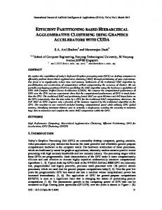
x1

x2

x3

x4

x5

x3

x4

x4

x5

x5

x5

Figure 9: A simple illustration for a five instance problem of how the triangle inequality can save distance computations worst-case, there may be no performance improvement. But in practice, one would expect the triangle inequality to have a beneficial effect and hence we can explore the best case and expected case results.

5.1

Best-case analysis for the γ-constraint

Consider the n points to cluster {x1 , ..., xn }. The first iteration of the agglomerative hierarchical clustering algorithm using symmetric distances is to compute the distance between each pair of points. This involves n(n − 1)/2 computations at the base level, namely d(x1 , x2 ), d(x1 , x3 ),..., d(x1 , xn ),..., d(xi , xi+1 ), d(xi , xi+2 ),...,d(xi , xn ),..., d(xn−1 , xn ). A simple example for n = 5 is shown in Figure 9. When using our γ-constraint, we first calculate the distance from the first instance x1 to all other instances (x2 , . . . , xn ) requiring n − 1 calculations. These distances provide us with estimates for the remaining (n − 1)(n − 2)/2 distances. In the best case, all of these lower bound distance estimates exceed γ and we save calculating all of these distances. We say that “these calculations are saved” since evaluating each distance exactly will require m floating point calculations while the lower bound uses just one floating point calculation. Thus in the best case there are only n − 1 distance computations at the bottom level of the dendrogram instead of n(n − 1)/2. For subsequent levels of the dendrogram no further distance calculations would be required in the best case.

5.2

Average-case analysis for using the γ-constraint

However, it is highly unlikely that the best case situation will ever occur. We now focus on average case analysis using first the Markov inequality and then the Chebyshev inequality to determine the expected performance improvement. In the conference version of this paper [8] we presented empirical results for improvements only at the bottom most level of the dendrogram. In this work, we provide experimental results to show that these bounds are useful for determining computational savings whilst constructing the entire dendrogram. 19

5.2.1

An expected-case performance upper bound based on Markov inequality

Let ρ be the average distance between any two instances in the data set to cluster. The triangle inequality provides a lower bound; if this bound exceeds γ, computational savings will result. We can bound how often this occurs if we can express γ in terms of ρ, hence let γ = cρ for some constant c > 1. Recall that the general form of the Markov inequality [17] is: P (X = x ≥ a) ≤ E(X)/a, where x is a value of the non-negative random variable X, a is a constant and E(X) is the expected value of X. Also, recall that at the base level of the dendrogram there are n(n − 1)/2 calculations and a possibility of saving at most (n − 1)(n − 2)/2 calculations. Since X is distance between two points chosen at random, E(X) = ρ and γ = a = cρ; we wish to determine how often the distance will exceed γ. Note that the population consists of all the data points whose mean pairwise distance is ρ. Therefore, by the Markov inequality, the probability that the distance will exceed γ is bounded by ρ/(cρ) = 1/c. At the lowest level of the dendrogram (k = n) where there are n(n − 1)/2 distance calculations, we notice that the expected number of times the triangle inequality will save us computation time is at most n(n − 1)/(2c). As indicated in Lemma 4.1, the total number of distance computations over the entire dendrogram is (n3 − n)/6 and so the the expected number of times the triangle inequality will save us computation time is at most (n3 − n)/(6c). Consider the 150 instance IRIS data set (n=150) where the average distance (with attribute value ranges all being normalized to between 0 and 1) between two instances is approximately 0.64; that is, ρ = 0.64. Suppose we choose γ = 2ρ = 1.28; that is, we do not wish to join clusters whose centroids are separated by a distance greater than 1.28. By not using the γ-constraint and the triangle inequality the total number of computations is (n3 − n)/6 = 562475. Using the constraint with γ = 1.28, the number of computations that are saved is at most 50%. How well this bound approximates the true improvement is empirically examined in the next section. 5.2.2

An expected-case performance upper bound based on Chebyshev inequality

Given a random variable X with expected value µ and variance σ 2 , the Chebyshev inequality states that P (|X − µ| ≥ γ) ≤ σ 2 /γ 2 (see for example, [17]). In our case, the random variable X represents distances between instances. In the following analysis, γ is a constant and is not a function of µ as before. To apply the Chebyshev inequality to our work, we first modify our distances so that µ = 0; note that this does not change σ 2 (which is a function of the second moment of the distribution). This can be achieved by calculating µ on the original data set and letting d′i,j = di,j − µ, ∀i, j. Applying the Chebyshev inequality with µ = 0, we have P (|X| ≥ γ) ≤ σ 2 /γ 2 . Since the event “X ≥ γ” implies the event “|X| ≥ γ”, we have P (X ≥ γ) ≤ P (|X| ≥ γ). Since the latter quantity is bounded by σ 2 /γ 2 , we get P (X ≥ γ) ≤ σ 2 /γ 2 . Thus, the expected fraction of the calculations that can be saved, as given by the Chebyshev’s inequality, is at most σ 2 /γ 2 .

20

This bound can be tightened in two ways, namely by making assumptions on the distribution of distances or by effectively estimating σ 2 for each level (without explicitly calculating it). For example, if the distribution of X was Gaussian, then symmetry would mean that P (X ≥ γ) = P (X ≤ −γ) and hence the performance bound could be tightened to σ 2 /(2γ 2 ).

5.3

Experimental results for the γ-constraint

We now empirically show that the γ-constraint can be used to improve efficiency and validate the usefulness of our bounds for our UCI data sets. We have chosen to plot distance calculations saved rather than raw computation time so as to allow more easy comparison and replication of our work. The raw computation time results show very similar trends since the overhead to check constraints is insignificant given our earlier complexity results. Our empirical results are shown in Figure 10. Of course, the Markov bound is generally the weaker of the two, but it is interesting to note that the Chebyshev bound is a strict and usually tight upper bound. In our experiments, the Chebyshev bound was occasionally (for the heart, ionosphere and image segmentation data sets) not as tight as in the other five cases. This is not due to data set size (all data sets are under 500 instances) but rather due to the number of dimensions. The heart, ionosphere and image segmentation data set have 22, 34 and 19 attributes respectively while the iris, wine, glass, protein and ecoli data sets have 4, 13, 20, 8 and 7 respectively. We expect the accuracy of the bound for these larger dimension data sets to improve when more instances are used since the estimates of µ and σ 2 obtained from the data will be more accurate.

5.4

Common distance measures for which γ-constraint can be used

The γ-constraint makes use of the triangle inequality and hence is only applicable for distance measures which satisfy that property. It is clear that the centroid distance measure obeys the triangle inequality, but what of the two other common measures, namely single-linkage and completelinkage? We now investigate this issue. Definition 5.2 Single and Complete Linkage Distance. Let de (x, y) denote the Euclidean distance between two points x and y and let πi and πj be two clusters. (a) The single-linkage distance between πi and πj is defined by dSL (πi , πj ) = argmina,b de (xa , xb ) : xa ∈ πi , xb ∈ πj . (b) The complete-linkage distance between πi and πj is defined by dCL (πi , πj ) = argmaxa,b de (xa , xb ) : xa ∈ πi , xb ∈ πj . Theorem 5.1 The complete-linkage distance in Definition 5.2 satisfies the triangle inequality but is not a distance metric.

21

Wine

Glass

Iris

1

1

1

0.8

0.8

0.8

0.6

0.6

0.6

0.4

0.4

0.4

0.2

0.2

0.2

0

0

0

0 0.2 0.4 0.6 0.8 1 1.2 1.4 1.6

0 0.2 0.4 0.6 0.8 1 1.2 1.4 1.6

0 0.2 0.4 0.6 0.8 1 1.2 1.4 1.6

Image Segmentation

Ecoli

Heart

1

1

1

0.8

0.8

0.8

0.6

0.6

0.6

0.4

0.4

0.4

0.2

0.2

0.2

0

0 0 0.2 0.4 0.6 0.8 1 1.2 1.4 1.6

0 0 0.2 0.4 0.6 0.8 1 1.2 1.4 1.6

Ionosphere

0 0.2 0.4 0.6 0.8 1 1.2 1.4 1.6 Protein

1

1

0.8

0.8

0.6

0.6

0.4

0.4

0.2

0.2

0

0 0 0.2 0.4 0.6 0.8 1 1.2 1.4 1.6

0 0.2 0.4 0.6 0.8 1 1.2 1.4 1.6

Figure 10: The percentage of distance calculations that are saved using the γ-constraints versus the value of γ. The solid line shows actual γ, the crosses show the Chebyshev upper bound and the crossed-line shows the Markov upper bound. 22

Proof: The four requirements for a metric D are: 1. d(x, y) ≥ 0 (non-negativity), 2. d(x, y) = 0 if and only if x = y (identity of indiscernibles), 3. d(x, y) = d(y, x) (symmetry) and 4. d(x, z) ≤ d(x, y) + d(y, z) (triangle inequality). Clearly Property 1 is satisfied for Euclidean distances. However, since the closest point to x is itself, dCL (πi , πi ) > 0 and hence Property 2 does not hold. Property 3 holds since since Euclidean distances are symmetric. We can prove Property 4 as follows. Let xai and xcl be the furthest points between Clusters a and c. Then d(xai , xcl ) ≤ d(xai , xb∗ ) + d(xb∗ , xcl ) where xb∗ is an arbitrary point in Cluster b. Now, d(xai , xb∗ )+d(xb∗ , xcl ) ≤ argmaxj,k d(xai , xbj )+ d(xbk , xcl ). Hence the triangle inequality holds. Theorem 5.2 The single linkage distance in Definition 5.2 does not satisfy the triangle inequality and hence is not a distance metric. Proof: To see that the single-linkage distance does not satisfy the triangle inequality, note that for an arbitrary point xb∗ , d(xai , xb∗ ) + d(xb∗ , xcl ) 6≤ argminj,k d(xai , xbj ) + d(xbk , xcl ). Therefore, centroid and complete-linkage distances satisfy the triangle inequality and can be used with the γ-constraint.

6

Conclusions

We have made several significant contributions to the new field of incorporating constraints into hierarchical clustering. We study four types of constraints, namely ML, CL, ǫ and δ. Our formal results for the feasibility problem (where the number of clusters is unspecified) show that clustering under all four types (ML, CL, ǫ and δ) of constraints is NP-complete; hence, creating a feasible dendrogram under all these is intractable but for all other constraint combinations the feasibility problem is tractable. These results are fundamentally different from our earlier work [7] not only because the feasibility problem and proofs are quite different but for non-hierarchical clustering many constraint combinations gave rise to an intractable feasibility problem. We have proved that under CL-constraints, traditional agglomerative clustering algorithms may give rise to a dead-end (irreducible) configuration. Even for data sets for which there are feasible solutions for all the values of k in the range kmin to kmax , traditional agglomerative clustering algorithms which start with kmax clusters and join two closest clusters may not get all the way to a feasible solution with kmin clusters. Therefore, the approach of joining the two nearest clusters may yield an incomplete dendrogram. 23

Our empirical results for incorporating constraints into agglomerative algorithms show that small amounts of constraints not only improve the label prediction error rates of dendrograms but also improve the run-time. The former is to be expected since a few initially carefully chosen joins can greatly improve the accuracy of the entire dendrogram. The latter is a particularly important result since agglomerative algorithms, though useful, are computationally time consuming; for large data sets, they may take Θ(n3 ) time. We showed that the number of distance calculations that are saved is a near linear function of the number of ML-constraints and the transitive nature of ML-constraints can greatly reduce the computation time. We presented a lower bound for this improvement. To further improve the efficiency of agglomerative clustering we introduced the γ-constraint which can be used in conjunction with triangle inequality to save computation time. The γconstraint allows a user to specify how far apart two cluster centroids should be. We derived best case and expected case analysis for this situation which were verified by our experiments. We showed that this constraint would work with the complete linkage and centroid linkage techniques but not with the single linkage approach which does not obey the triangle inequality. Finally, we provided both Markov and Chebyshev upper bounds on the distance calculations that will be saved. Our experimental results clearly showed the following interesting insights. • Adding ML- and CL-constraints to hierarchical clustering can achieve significantly better improvements in accuracy. This is to be expected given that a few carefully selected joins can greatly improve the accuracy of the overall dendrogram. • Adding ML- and CL-constraints can significantly reduce the number of distance calculations. We presented a simple lower bound that estimates how many distance calculations will be saved. • The γ-constraint can greatly reduce the number of distance calculations in the expected case and the validation of the performance of our Markov and Chebyshev bounds showed that the latter is a useful upper bound.

7

Acknowledgments

We thank the reviewers for their careful reading of the manuscript and for providing valuable suggestions. The first author gratefully acknowledges support of this work by NSF grant number IIS-0801528 titled “CAREER: Knowledge Enhanced Clustering using Constraints”.

24

8

Appendix A

Proof of Theorem 3.1 It is easy to see that Fhc is in NP since one can guess a partition of S into clusters and verify that the partition satisfies all the given constraints. We establish NP-hardness by a reduction from Opl. A note regarding terminology: In this proof, we use the term ‘nodes’ to refer to the points which are to be clustered. We need this terminology since the term ‘instance’ must be used in its complexity theoretic sense in the proof. Given an instance I of the Opl problem consisting of variable set X and clause set Y , we create an instance I ′ of the Fhc problem as follows. We first describe the nodes in the instance I ′ . For each Boolean variable xi , we create a node vi , 1 ≤ i ≤ n. Let V = {v1 , v2 , . . . , vn }. For each clause yj = {xj1 , xj2 , xj3 }, 1 ≤ j ≤ m, we do the following: (a) We create a set Aj = {wj1 , wj2 , wj3 } containing three nodes. (The reader may find it convenient to think of nodes wj1 , wj2 and wj3 as corresponding to the variables xj1 , xj2 and xj3 respectively.) We refer to the three nodes in Aj as the primary nodes associated with clause yj . (b) We create six additional nodes denoted by a1j , a2j , b1j , b2j , c1j and c2j . We refer to these six nodes as the secondary nodes associated with clause yj . For convenience, we let Bj = {a1j , b1j , c1j }. Also, we refer to a2j , b2j and c2j as the twin nodes of a1j , b1j and c1j respectively. Thus, the construction creates a total of n + 9m nodes. The distances between these nodes are chosen in the following manner, by considering each clause yj , 1 ≤ j ≤ n. (a) Let the primary nodes wj1 , wj2 and wj3 associated with clause yj correspond to Boolean variables xp , xq and xr respectively. Then d(vp , wj1 ) = d(vq , wj2 ) = d(vr , wj3 ) = 1. (b) The distances among the primary and secondary nodes associated with yj are chosen as follows. (i) d(a1j , a2j ) = d(b1j , b2j ) = d(c1j , c2j ) = 1. (ii) d(a1j , wj1 ) = d(a1j , wj2 ) = 1. (iii) d(b1j , wj2 ) = d(b1j , wj3 ) = 1. (iv) d(c1j , wj1 ) = d(c1j , wj3 ) = 1. For each pair of nodes which are not covered by cases (a) or (b), the distance is set to 2. The constraints are chosen as follows. 25

(a) ML-constraints: For each j, 1 ≤ j ≤ n, there are the following ML-constraints: ML(wj1 , wj2 }), ML(wj1 , wj3 ), ML(wj2 , wj3 ), ML(a1j , a2j ), ML(b1j , b2j ) and ML(c1j , c2j ). (b) CL-constraints: (i) For each pair of nodes vp and vq , there is a CL-constraint CL(vp , vq ). (ii) For each j, 1 ≤ j ≤ m, there are three CL-constraints, namely CL(a1j , b1j ), CL(a1j , c1j ) and CL(b1j , c1j ). (c) ǫ-constraint: The value of ǫ is set to 1. This completes the construction of the Fhc instance I ′ . It can be verified that the construction can be carried out in polynomial time. We now prove that the Fhc instance I ′ has a solution if and only if the Opl instance I has a solution. If part: Suppose the Opl instance I has a solution. Suppose this solution assigns the value true to variables xi1 , xi2 , . . ., xir and the value false to the rest of the variables in X. A solution to the Fhc instance I ′ is obtained as follows. (a) Recall that V = {v1 , v2 , . . . , vn } and that {vi1 , vi2 , . . . , vir } represents the the set of nodes corresponding to the variables which were assigned the value true. For each node v in V − {vi1 , vi2 , . . . , vir }, create the singleton cluster {v}. (b) For each node viq corresponding to variable xiq , which has been assigned the value true (1 ≤ q ≤ r), we create the following clusters. Let yj1 , yj2 , . . ., yjp be the clauses in which variable xiq occurs. (i) Create one cluster containing the following nodes: node viq , the three primary nodes corresponding to each clause yjl , 1 ≤ l ≤ p, and one pair of secondary nodes corresponding to cluster yjl chosen as follows. Since xiq satisfies clause yjl , one primary node corresponding to clause yjl has viq as its ǫ-neighbor. By our construction, exactly one of the secondary nodes corresponding to yjl , say a1jl , is an ǫ-neighbor of the other two primary nodes corresponding to yjl . The cluster containing viq includes a1jl and its twin node a2jl . (ii) For each clause yjl , 1 ≤ l ≤ p, the cluster formed in (i) does not include two secondary nodes and their twins. Each secondary node and its twin is put in a separate cluster. (Thus, this step creates 2p additional clusters.) We claim that the clusters created above satisfy all the constraints. To see this, we note the following. 26

(a) ML-constraints are satisfied because of the following: the three primary nodes corresponding to each clause are in the same cluster and each secondary node and its twin are in the same cluster. (b) CL-constraints are satisfied because of the following: each node corresponding to a variable appears in a separate cluster and exactly one secondary node (along with its twin) corresponding to a variable appears in the cluster containing the three primary nodes corresponding to the same variable. (c) ǫ-constraints are satisfied because of the following. (Note that singleton clusters can be ignored here.) (i) Consider each non-singleton cluster containing a node vi corresponding to Boolean variable xi . Let yj be a clause in which xi appears. Node vi serves as the ǫ-neighbor for one of the primary nodes corresponding to yj in the cluster. One of the secondary nodes, corresponding to yj , say a1j , serves as the ǫ-neighbor for the other two primary nodes corresponding to yj as well as its twin node a2j . (ii) The other non-singleton clusters contain a secondary node and its twin. These two nodes are ǫ-neighbors of each other. Thus, we have a feasible clustering for the instance I ′ . Only if part: Suppose the Fhc instance I ′ has a solution. We can construct a solution to the Opl instance I as follows. We begin with a proposition. Proposition 8.1 Consider any clause yj . Recall that Aj = {wj1 , wj2 , wj3 } denotes the set of three primary nodes corresponding to yj . Also recall that V = {v1 , v2 , . . . , vn }. In any feasible solution to I ′ , the nodes in Aj must be in the same cluster, and that cluster must also contain exactly one node from V . Proof of proposition: The three nodes in Aj must be in the same cluster because of the MLconstraints involving them. The cluster containing these three nodes may include only one node from the set Bj = {a1j , b1j , c1j } because of the CL-constraints among these nodes. Each node in Bj has exactly two of the nodes in Aj as its ǫ-neighbor. Note also that the only ǫ-neighbors of each node in Aj are two of the nodes in Bj and one of the nodes from the set V = {v1 , v2 , . . . , vn }. Thus, to satisfy the ǫ-constraint for the remaining node in Aj , the cluster containing the nodes in Aj must also contain at least one node from V . However, because of the CL-constraints between each pair of nodes in V , the cluster containing the nodes in Aj must have exactly one node from V . This completes the proof of the claim.

27

Proposition 8.2 Consider the following truth assignment to the variables in the instance I: Set variable xi to true if and only if node vi appears in a non-singleton cluster. This truth assignment sets exactly one literal in each clause yj to true. Proof of proposition: From Proposition 8.1, we know that the cluster containing the three primary nodes corresponding to yj contains exactly one node from the set V = {v1 , v2 , . . . , vn }. Let that node be vi . Thus, vi is the ǫ-neighbor of one of the primary nodes corresponding to yj . By our construction, this means that variable xi appears in clause yj . Since xi is set to true, clause yj is satisfied. Also, note that the cluster containing vi does not include any other node from V . Thus, the chosen truth assignment satisfies exactly one of the literals in yj . From Proposition 8.2, it follows that the instance I has a solution, and this completes the proof of Theorem 3.1.

28

References [1] E. Bae and J. Bailey, “COALA : A Novel Approach for the Extraction of an Alternate Clustering of High Quality and High Dissimilarity”, Proc. 6th IEEE International Conference on Data Mining (ICDM 2006), Hong Kong, Dec. 2006, pp. 53–62. [2] S. Basu, A. Banerjee and R. Mooney, “Semi-supervised Clustering by Seeding”, Proc. 19th International Conference on Machine Learning (ICML 2002), Sydney, Australia, Jul. 2002, pp. 27–34. [3] S. Basu, M. Bilenko and R. J. Mooney, “Active Semi-Supervision for Pairwise Constrained Clustering”, Proc. 4th SIAM International Conference on Data Mining (SDM 2004), Lake Buena Vista, FL, Apr. 2004, pp. 333–344. [4] S. Basu, I. Davidson and K. Wagstaff, Advances in Clustering with Constraints: Algorithms, Theory and Practice, Chapman & Hall, CRC Press, 2008 (to appear). [5] T. Cormen, C. E. Leiserson, R. Rivest and C. Stein, Introduction to Algorithms, MIT Press, Cambridge, MA, 2001. [6] I. Davidson, M. Ester and S. S. Ravi, “Efficient Incremental Clustering with Constraints”, Proc. ACM Conference of Knowledge Discovery and Data Mining (KDD 2007), San Jose, CA, Aug. 2007, pp. 240–249. [7] I. Davidson and S. S. Ravi, “Clustering with Constraints: Feasibility Issues and the k-Means Algorithm”, Proc. SIAM International Conference on Data Mining (SDM 2005), Newport Beach, CA, Apr. 2005, pp. 138–149. [8] I. Davidson and S. S. Ravi, “Agglomerative Hierarchical Clustering With Constraints: Theoretical and Empirical Results”, Proc. 15th European Conference on Principles and Practice of Knowledge Discovery in Databases (PKDD 2005), Porto, Portugal, Oct. 2005, pp. 59–70. [9] I. Davidson and S. S. Ravi, “Identifying and Generating Easy Sets of Constraints For Clustering”, Proc. 21st National Conference on Artificial Intelligence (AAAI 2006), Boston, MA, Jul. 2006. [10] I. Davidson and S. S. Ravi, “The Complexity of Non-Hierarchical Clustering with Instance and Cluster Level Constraints”, Data Mining and Knowledge Discovery, Vol. 14, No. 1, Feb. 2007, pp. 25–61. [11] I. Davidson and S. S. Ravi, “Intractability and Clustering with Constraints”, Proc. International Conference on Machine Learning (ICML 2007), Portland, OR, June 2007, pp. 201–208. [12] I. Davidson, K. Wagstaff, S. Basu, “Measuring Constraint-Set Utility for Partitional Clustering Algorithms”, Proc. 16th European Conference on Principles and Practice of Knowledge Discovery in Databases (PKDD 2006), Berlin, Germany, Sept. 2006, pp. 115–126. [13] L. Dragomirescu and T. Postelnicu, “A Natural Agglomerative Clustering Method for Biology”, Biometrical Journal, Vol. 33, Issue 7, 2007, pp. 841–849. [14] C. Elkan, “Using the Triangle Inequality to Accelerate k-Means”, Proc. International Conference on Machine Learning (ICML 2003), Washington, DC, Aug. 2003, pp. 147–153. 29

[15] R. L. Graham, D. E. Knuth and O. Patashnik, Concrete Mathematics: A Foundation for Computer Science, Addison-Wesley, Reading, MA, 1989. [16] D. Klein, S. D. Kamvar and C. D. Manning, “From Instance-Level Constraints to Space-Level Constraints: Making the Most of Prior Knowledge in Data Clustering”, Proc. International Conference on Machine Learning (ICML 2002), Sydney, Australia, Jul. 2002, pp. 307–314. [17] M. Mitzenmacher and E. Upfal, Probability and Computing: Randomized Algorithms and Probabilistic Analysis, Cambridge University Press, New York, NY, 2005. [18] P. Mohanta, D. Mukherjee and S. Acton, “Agglomerative Clustering for Image Segmentation”, Proc. International Conference on Pattern Recognition (ICPR 2002), Qubec City, Canada, Aug. 2002, pp. 664–667. [19] M. Nanni, “Speeding-up Hierarchical Agglomerative Clustering in Presence of Expensive Metrics”, Proc. 9th Pacific Asia Conference on Knowledge Discovery and Data Mining (PAKDD 2005), Hanoi, Vietnam, May 2005, pp. 378–387. [20] T. J. Schaefer, “The Complexity of Satisfiability Problems”, Proc. 10th ACM International Symposium on Theory of Computing (STOC 1978), San Diego, CA, May 1978, pp. 216–226. [21] K. Wagstaff and C. Cardie, “Clustering with Instance-Level Constraints”, Proc. 17th International Conference on Machine Learning (ICML 2000), Stanford, CA, Jun.-Jul. 2000, pp 1103– 1110. [22] K. Wagstaff, C. Cardie, S. Rogers and S. Schroedl, “Constrained K-means Clustering with Background Knowledge”, Proc. 18th International Conference on Machine Learning (ICML 2001), Williamstown, MA, Jun.-Jul. 2001, pp. 577–584. [23] E. Xing, A. Ng, M. Jordan and S. Russell, “Distance Metric Learning with Application to Clustering with Side-Information”, Advances in Neural Information Processing Systems (NIPS 2002), Vol. 15, Vancouver, Canada, Dec. 2002, pp. 505–512. [24] Y. Zho and G. Karypis, “Hierarchical Clustering Algorithms for Document Datasets”, Data Mining and Knowledge Discovery, Vol. 10 No. 2, Mar. 2005, pp. 141–168.

30