Physical source realization of complex source pulsed beams Ehud Heymana) and Vitality Lomakin Department of Electrical Engineering-Physical Electronics, Tel-Aviv University, Tel-Aviv 69978, Israel
Gerald Kaiserb) The Virginia Center for Signals and Waves, 1921 Kings Road, Glen Allen, Virginia 23060
共Received 24 June 1999; accepted for publication 21 December 1999兲 Complex source pulsed beams 共CSPB兲 are exact wave-packet solutions of the time-dependent wave equation that are modeled mathematically in terms of radiation from a pulsed point source located at a complex space–time coordinate. In the present paper, the physical source realization of the CSPB is explored. This is done in the framework of the acoustic field, as a concrete physical example, but a similar analysis can be applied for electromagnetic CSPB. The physical realization of the CSPB is addressed by deriving exact expressions for the acoustic source distribution in the real coordinate space that generates the CSPB, and by exploring the power and energy flux near these sources. The exact source distribution is of finite support. Special emphasis is placed on deriving simplified source functions and parametrization for the special case where the CSPB are well collimated. © 2000 Acoustical Society of America. 关S0001-4966共00兲00804-3兴 PACS numbers: 43.20.Px, 43.20.Bi, 41.20.Jb, 03.50.⫺z 关ANN兴
INTRODUCTION
Complex source pulsed beams 共CSPB兲 关also termed pulsed beams 共PB兲 or isodiffracting PB兴 are exact wavepacket solutions of the time-dependent wave equation that can be modeled mathematically in terms of radiation from a pulsed point source located at a complex space–time coordinate.1–3 Their properties, namely their direction, collimation, and space–time width, are determined by the complex source coordinates. Physically, however, these solutions are generated by physical source distributions 共derived in this paper兲; hence, the complex source model may be considered as a mathematical trick to obtain compact field solutions due to these source distributions. This complex source approach has been originally introduced in the context of time-harmonic fields.4–7 Another approach to derive the CSPB has been derived independently in Ref. 8. The CSPB have many properties that make them favorable wave objects within a general wave-based approach for forward and inverse problems: 共1兲 They are convenient wavelets for high-resolution probing of the propagation environment, and may be used to selectively excite local scattering and diffraction phenomena 共see items 2 and 4 below兲. 共2兲 They provide benchmark solutions for scattering of collimated wave packets by canonical configurations,9–11 for propagation in inhomogeneous media,12,13 in dispersive media,14–16 and in random media,17,18 or can used to model practical systems involving collimated short-pulse fields.19–22 共3兲 They furnish a complete basis for local observable-based spectral synthesis of general transient fields, providing a priori localization 共since only those PB propagators that pass near the space–time observation point need to be a兲
Electronic mail:
[email protected] Electronic mail:
[email protected]
b兲
1880
J. Acoust. Soc. Am. 107 (4), April 2000
accounted for兲. Several expansion schemes which apply to different source configurations have been derived in Refs. 23–28. 共4兲 Finally, in view of these properties the CSPB are wellsuited to wave-based data processing and local inverse scattering.29,30 The space–time localization described above provides a systematic wave-based approach for dealing with global complexity. Concentrating on localized solutions permits the use of specific well-defined ‘‘simpler’’ problems from which global solutions are assembled. The CSPBs not only provide simple local wave solutions, but may also be directed in space–time to interrogate a particular subenvironment or wave phenomenon in the global conglomerate. Other classes of wave-packet solutions in free space have been introduced in various disciplines. The basic ones are: solutions based on Brittingham’s ‘‘focus wave modes,’’ 31–34 ‘‘nondiffracting beams’’ or ‘‘X-waves’’ 35,36 and ‘‘bullet’’-type solutions.37,38 These solutions have not yet been utilized in a full ‘‘wave-based architecture’’ as described above. As has been pointed out previously, the CSPB can be generated by a finite distribution of physical sources.2 Our aim in the present paper is to explore this physical source realization. This is done here within the framework of the acoustic field which provides a concrete physical example, but a similar analysis can be applied for electromagnetic CSPB. The physical realization of the CSPB is addressed by deriving expressions for the acoustic source distributions and by exploring the power and energy flux around these sources. The finite support source functions obtained give rise to the globally exact CSPB. Yet, from a practical point of view, as discussed in the preceding paragraph, special emphasis is given to the parameter range where the CSPB are well collimated so that they maintain their localized wave-packet structure while propagating in the ambient en-
0001-4966/2000/107(4)/1880/12/$17.00
© 2000 Acoustical Society of America
1880
vironment. In this special case the CSPB can be realized effectively by a truncated source distribution whose spatial support is much smaller than that of the exact CSPB. The collimated PB fields generated by the truncated aperture resemble the exact CSPB near the beam axis, but deviate from it in far off-axis region, where they are both negligible anyway. The presentation starts with a brief summary of the relevant acoustic field equations 共Sec. I兲 and of the basic properties of the CSPB 共Sec. II兲. The physical realization is then explored in Sec. III from the point of view of the power and energy flow. The expressions for the source distributions are then derived in Secs. IV and V, starting with the formulation of general schemes for constructing source realizations and then applying them to calculate the CSPB sources. The presentation ends with a summary and conclusions. I. ACOUSTIC FIELDS AND SOURCES
The linear acoustic equations for the pressure field p(r,t) and velocity field v(r,t) at the space–time point r ⫽(x,y,z)苸R3 and time t苸R are 1 p⫹ⵜ•v⫽ , c 2% t
共1.1a兲
% t v⫹ⵜp⫽f,
共1.1b兲
where (r,t) and f(r,t) represent the scalar particle injection source distribution and the force distribution, respectively. Here, c⫽1/冑 % is the wave speed in the medium, with and % being the compressibility and density, respectively. In this paper we consider radiation in a uniform medium and, without loss of generality, we assume that %⫽1. Henceforth, we use boldface type to denote vector constituents and a ° over a vector to denote a unit vector. Assuming sources bounded in a volume V of finite support, the integral solution of 共1.1兲 is p⫽
冕
V
d3 ⬘
冋
册
1 1 ˚ ⫹ 1 关 f兴 • , 关 ˙ 兴 ⫹ 关 ˙f兴 •R 4R c R
共1.2兲
˚ and 关 F 兴 denotes the retarded value where R⫽r⫺r⬘ ⫽RR F(r⬘ ,t ⬘ ) 兩 t ⬘ ⫽t⫺R/c for any function F(r⬘ ,t ⬘ ). Here and henceforth, overdots and overcircles denote time derivatives and unite vectors, respectively. The solution for v is readily inferred from p. II. COMPLEX SOURCE PULSED BEAMS „CSPB…
共2.1兲
where r⬘ 苸R3 and t ⬘ 苸R define the space–time source coordinates and is a given time signal. From 共1.2兲, the solution is p 共 r,t 兲 ⫽ 共 t⫺t ⬘ ⫺R/c 兲 /R.
共2.2兲
The CSPB is modeled analytically by extending the source coordinates (r⬘ ,t ⬘ ) in 共2.1兲 into the complex domain. These coordinates may be expressed in general as 1881
J. Acoust. Soc. Am., Vol. 107, No. 4, April 2000
共2.3a兲
t ⬘ ⫽t r⬘ ⫹it ⬘i ,
t i⬘ ⭓b/c,
共2.3b兲
where r0 is a real coordinate point that defines the center of the beam waist, b is a real vector that defines the beam direction, and b⬎0 is a constant which is interpreted as the collimation distance of the beam 关see the discussion after 共2.19兲兴. The condition on t ⬘i in 共2.3b兲 will be explained after 共2.13兲. Without loss of generality, we shall assume henceforth that r0 ⫽0 and b⫽z˚b, i.e.,
r⬘ ⫽ 共 0,0,ib 兲 ,
t ⬘ ⫽ib/c.
共2.4a兲 共2.4b兲
B. Properties of the complex distance s „r…
In order to extend 共2.2兲 to the complex source case, we must first extend the definition of the distance R of the observer from the source. We define this distance as s 共 r兲 ⬅ 冑共 x⫺x ⬘ 兲 2 ⫹ 共 y⫺y ⬘ 兲 2 ⫹ 共 z⫺z ⬘ 兲 ,
共2.5a兲
⫽ 冑 2 ⫹ 共 z⫺ib 兲 2 ,
共2.5b兲
⫽s r ⫹is i ,
共2.5c兲
where 共2.5a兲 is the general definition while 共2.5b兲 corresponds to the special choice of the complex source coordinates in 共2.4a兲, with ⫽ 冑x 2 ⫹y 2 . The branch of the complex root in 共2.5兲 is chosen with 共2.6兲
Re s⬎0.
This choice implies that s→r as b/r→0 关see 共2.21兲兴. Other properties of s will be discussed next, where without loss of generality we consider the choice of (r⬘ ,t ⬘ ) in 共2.4兲. The set of branch points of s in R3 is the circle B in the z⫽0 plane, defined by 冑x 2 ⫹y 2 ⫽b. In order for s(r) to be a single-valued function of r, we choose a branch cut in R3 . The choice implied by 共2.6兲 is a flat disk 共Fig. 1兲 E0 ⫽ 兵 r:x 2 ⫹y 2 ⭐b 2 ,z⫽0 其 ,
共2.7兲
although any continuous deformation of E0 leaving its boundary B invariant will do the same. The real and imaginary parts of s⫽s r ⫹is i have distinct physical roles. They can also be used as the natural coordinate system for the CSPB. For a given point r苸R3 , one finds
where s r ⬎0,⫺b⬍s i ⬍b.
Let the source in 共1.1兲 be
˙ ⫽4 ␦ 共 r⫺r⬘ 兲 共 t⫺t ⬘ 兲 ,
兩 b兩 ⫽b,
共 ,z 兲 ⫽b ⫺1 共 冑b 2 ⫹s r2 冑b 2 ⫺s 2i ,⫺s r s i 兲 ,
A. The complex source coordinates
f⫽0,
r⬘ ⫽r0 ⫹ib,
共2.8兲
Equation 共2.8兲 defines an oblate spheroidal 共OS兲 system (s r ,s i , ) with ⫽tan⫺1(y/x) 共see Fig. 1兲: The surfaces s r ⫽const are spheroids Es r Es r :
x 2 ⫹y 2 b 2 ⫹s r2
⫹
z2 s r2
⫽1,
s r ⬎0.
共2.9兲
In the limit s r →0, Es r shrinks to E0 , whereas for s r Ⰷb it tends to a sphere with radius s r ⫽r. Similarly, s i ⫽const. define a family of one-sided hyperboloids Hs i Heyman et al.: Physical source realization of pulsed beams
1881
Since ⫺b⭐s i ⭐b 关see 共2.10兲兴 it follows that Im ⭐0 for all ⫹
real (r,t) as required by the analyticity of . Recalling further that s(r) is continuous everywhere in R3 except across the disk E0 关see the discussion in connection with 共2.7兲兴, it ⫹
follows that p is an exact homogeneous solution of the timedependent wave equation everywhere except for E0 , which is henceforth referred to as the ‘‘source disk’’ since it represents the location of the real sources that give rise to the solution in 共2.12兲 共see Sec. V兲. The solution in 共2.12兲 has the general properties of a PB 共a collimated space–time wave-packet兲 that emerges from r0 共here, the origin兲 and propagates along the beam axis b 共here, the positive z-axis兲. Confinement along the beam axis is af⫹
FIG. 1. The oblate spheroidal 共OS兲 coordinate system. The shaded areas are the regions D in( ) defined in 共3.16兲 where the energy flows inward with respect to the OS system. The light- and dark-shaded areas correspond to frequencies kb⫽0.7 and kb⫽1.1, respectively.
Hs i :
x 2 ⫹y 2
z2
b 2 ⫺s i
s 2i
⫺ 2
⫽1,
⫺b⭐s i ⭐b.
共2.10兲
These hyperboloids intersect the z⫽0 plane at E0 , and are discontinuous there with s i 兩 z⫽⫾0 ⫽⫿ 冑b 2 ⫺ 2 .
共2.11兲
For ⫺b⭐s i ⭐0, Hs i covers the domain z⬎0: It shrinks to the positive z axis for s i ⫽⫺b and as s i →0, it tends to the complement of E0 in the plane z⫽0. For 0⭐s i ⭐b, it likewise covers the domain z⬍0. Other properties of the OS system are mentioned in 共2.16兲, 共2.21兲, and in Appendix B.
The field due to the complex source in 共2.3兲 is obtained as an analytic extension of the real source solution in 共2.2兲. In order to deal with the complex propagation delays from the complex source coordinate to the real space–time observation point, one should use analytic signals that can accommodate complex time variables 共see Appendix A兲. Henceforth, analytic signals will be denoted by the symbol ⫹. The real field is then obtained by taking the real part of the analytic field solution 关in fact, one may also take the imaginary part of the analytic field; see discussion after 共A3兲兴. The analytic pressure field at a real space–time observation point (r,t), obtained as an analytic extension of 共2.2兲, is given by ⫹
p 共 r,t 兲 ⫽ 共 兲 /s,
⫽t⫺ ␥ 共 r兲 ,
共2.12兲
with
␥ ⫽t ⬘ ⫹s/c, ⫽s r /c⫹i 共 b⫹s i 兲 /c⫽ ␥ r ⫹i ␥ i ,
共2.13a兲 共2.13b兲
where 共2.13b兲 applies for the choice of t ⬘ in 共2.4b兲. The functions ␥ r,i (r) are the real and imaginary time delays. 1882
J. Acoust. Soc. Am., Vol. 107, No. 4, April 2000
⫹
on: 共a兲 the rate of decay of in the lower half of the complex plane 共that typically depends on the pulse length兲, and 共b兲 on the rate of increase of Im in 共2.13兲 away from the z axis 关following the discussion in 共2.10兲, Im vanishes on the positive z axis and increases away from it兴. The weakest signal is obtained along the negative z axis where Im ⫽⫺2b/c. Thus, the ellipsoids Es r of 共2.9兲 are the wavefronts associated with the time-delay ␥ r ⫽s r /c, while the hyperboloids Hs i of 共2.10兲 are equi-amplitude surfaces. 1. Parametrization of the real signal
To further understand the properties of the real PB field, we introduce the real signal ␥ i (t) and its Hilbert transform ¯ ␥ (t) via 关see 共A3兲兴 i ⫹
C. The CSPB solution
⫹
fected by the pulse shape of while transverse confinement is due to the general property of analytic signals which decay in the lower half of the complex plane as the imaginary part of becomes negative. Thus, the beamwidth depends
共 t⫺i ␥ i 兲 ⫽ ␥ i 共 t 兲 ⫹i ¯ ␥ i 共 t 兲 ,
t苸R.
共2.14兲
One finds that ⫹
p⫽Re p ⫽ 关 s r ␥ i 共 t⫺ ␥ r 兲 ⫹s i ¯ ␥ i 共 t⫺ ␥ r 兲兴 / 兩 s 兩 2 ,
共2.15兲
where from 共2.13b兲 ␥ r ⫽s r /c and ␥ i ⫽(b⫹s i )/c. Thus, along a given hyperboloid Hs i 关see 共2.10兲兴, the signal is gradually Hilbert transformed from ¯ ␥ (t⫺ ␥ r )/s i in the near i
zone, where s r →0, to ␥ i (t⫺ ␥ r )/s r in the far zone, where s r ⬃rⰇb. 2. Paraxial parametrization for collimated PBs
Points near the positive beam axis, where the PB is strong, are of particular importance. From 共2.5b兲 and 共2.6兲 we have for Ⰶ 冑z 2 ⫹b 2 , s⯝⫹ 关共 z⫺ib 兲 ⫹ 21 2 / 共 z⫺ib 兲兴 ,
z0
共2.16兲
共note the discontinuity at E0 ). Substituting this into 共2.12兲, the field near the positive z axis is given by ⫹
⫹
p 共 r,t 兲 ⫽ 共 t⫺z/c⫺ 21 2 /c 共 z⫺ib 兲兲 / 共 z⫺ib 兲 .
Heyman et al.: Physical source realization of pulsed beams
共2.17兲 1882
To parametrize this field, we write 1/(z⫺ib)⫽1/R(z) ⫹i/I(z), where R 共 z 兲 ⫽z⫹b 2 /z,
I 共 z 兲 ⫽b 共 1⫹ 共 z/b 兲 2 兲 ,
共2.18兲
thereby obtaining from 共2.13兲 共2.19兲
Thus, R(z) is identified as the radius of curvature of the PB wavefront, while I(z) controls the paraxial decay away from the axis. For zⰆb,I(z) is to leading order independent of z and the PB propagates essentially without decay or spreading, while for zⰇb, ␥ i ⬃(b/2c)( /z) 2 , and the wave packet diverges along the cones /z⫽const. 关see 共2.25兲兴. The real PB field along the z axis is given now by p⫽ 关 z ␥ i 共 t⫺ ␥ r 兲 ⫺b ¯ ␥ i 共 t⫺ ␥ r 兲兴 / 关 z 2 ⫹b 2 兴 ,
共2.20兲
where ␥ r,i are now given in 共2.19兲. Thus, in the near zone, the real signal is dominated by ⫺b ⫺1 ¯ ␥ i (t⫺ ␥ r ), but as z increases, it is gradually Hilbert transformed, and finally for zⰇb it is dominated by z ⫺1 ␥ i (t⫺ ␥ r ). 3. Far-field pattern
Another important limit occurs in the far zone for rⰇb where from 共2.5b兲 cos ⫽z/r.
共2.21兲
Substituting this into 共2.12兲, we obtain ⫹
⫹
p 共 r,t 兲 ⫽r ⫺1 共 t⫺r/c⫺i ␥ i 共 兲兲 ,
␥ i 共 兲 ⫽ 共 1⫺cos 兲 b/c. 共2.22兲
The function Re ⫹(t⫺␥i()) is the time-dependent radiation pattern. It is strongest for ⫽0 and decays to a minimum at ⫽ 关see the diffraction angle ⌰ in 共2.27兲兴. 4. Example: Analytic ␦ PB
The PB solutions may accommodate any analytic pulse shape. It is useful at this stage to consider an example of a particular pulse shape, namely the n-times differentiated analytic-␦ pulse ⫹
⫹
共 t 兲 ⫽ ␦ 共 n 兲 共 t⫺i 21 T 兲 ⫽
共 ⫺ 兲 n! n
i 共 t⫺i T 兲 1 2
, n⫹1
T⬎0.
共2.23兲
It is sometimes convenient to multiply the pulses in 共2.23兲 by e i ␣ with 0⭐ ␣ ⬍ in order to change the balance between the signal and its Hilbert transform when one considers the real part of the field. The parameter T in 共2.23兲 is a measure of the pulse length. The spectrum of these pulses is ˆ ( ) ⫽(⫺i ) n e ⫺ T/2 for ⬎0. The derivatives suppress the low frequencies and thus create a more localized 共fasterdecaying兲 PB in both the axial and transversal directions. In many applications, using n⭓2 is required because of the higher collimation properties of the resulting PB.26,30 Furthermore, as will be discussed in Sec. III 关see 共3.16兲兴, PB with frequency components below ⬍c/b are difficult to excite. 1883
1 2
⫹
␥ r ⫽z/c⫹ 2 /2cR 共 z 兲 , ␥ i ⫽ 2 /2cI 共 z 兲 .
s⯝r⫺ib cos ,
For simplicity, however, we discuss here the PB properties for the case n⫽0 and ␣ ⫽0. The real waveforms in 共2.14兲 are given by
J. Acoust. Soc. Am., Vol. 107, No. 4, April 2000
␥ i 共 t 兲 ⫽Re ␦ 共 t⫺i 共 21 T⫹ ␥ i 兲兲 ⫽ ⫺1
T⫹ ␥ i
t ⫹ 共 21 T⫹ ␥ i 兲 2 2
⫹
¯ ␥ 共 t 兲 ⫽Im ␦ 共 t⫺i 共 21 T⫹ ␥ i 兲兲 ⫽⫺ ⫺1 i
t t ⫹ 共 T⫹ ␥ i 兲 2 2
1 2
共2.24a兲
,
. 共2.24b兲
For a given ␥ i , the half-amplitude pulse width in 共2.24a兲 is (T⫹2 ␥ i ) and the peak amplitude 共at t⫽0) is ⫺1 ( 21 T ⫹ ␥ i ) ⫺1 . Thus, the waveform is strongest and shortest for ␥ i ⫽0 共the beam axis兲, and decays as ␥ i grows away from the axis. The half-amplitude beamwidth is therefore obtained when ␥ i ⫽ 21 T. Substituting 共2.19兲 for ␥ i in the paraxial zone, the beam diameter is found to be W 共 z 兲 ⫽W 0 冑1⫹ 共 z/b 兲 2 ,
W 0 ⫽2 冑cTb.
共2.25兲
One observes that for 0⬍z⬍b the beamwidth remains essentially constant, while for zⰇb it opens up along a diffraction cone whose angle ⌰⬅W(z)/z is parametrized by ⌰ ⫽2 冑cT/b. Collimated PB with ⌰Ⰶ1 are obtained when 共2.26兲
cT/bⰆ1.
Note also that, under this collimation condition, the effective width of the source distribution, which is roughly given by W 0 关see 共2.25兲兴, is much narrower than the ‘‘exact’’ source disk E0 whose radius is b. One obtains the following rule of thumb for the relation between the pulse length T, the beamwidth at the waist W 0 , the diffraction angle ⌰, and the collimation distance b 共 W 0 /b 兲 2 ⫽⌰ 2 ⫽4cT/bⰆ1.
共2.27兲
Thus, the field properties are controlled by the PB parameter cT/b. Similar properties are obtained for other pulse types, such as nonmodulated or modulated Gaussian pulses or modulated ␦ pulses. Figure 2 depicts cross sectional snapshots in the (z, ) plane of the axially symmetric p field of 共2.12兲. The pulse used
is
⫹
a
differentiated
analytic
delta
pulse
⫹
(t)
⫽⫺e i ␣ ␦ (1) (t⫺i 21 T) of type 共2.23兲 and a PB parameter cT/b⫽10⫺3 that yields a collimated PB 关see 共2.26兲兴. 共Recall that it is advantageous to deemphasize the low frequencies ⫹
further by using ␦ (2) and a smaller parameter cT/b.) As mentioned in 共2.23兲, the term e i ␣ is used to change the balance between the signal and its Hilbert transform. Here, ␣ has been chosen to be /3, which provides the ‘‘nicest’’ result 共this value also provides the clearest results of the power flux analysis in Fig. 3兲. The field in Fig. 2 is plotted at times ct/b⫽0.2, 1, and 2, where the PB is localized, respectively, in the near zone z ⫽0.2b, at the collimation distance z⫽b, and in the ‘‘far’’ zone z⫽2b. Note the Hilbert transform exhibited by the waveforms in the transition from the near to the far zones 关recall 共2.15兲 and 共2.20兲兴. To demonstrate the effect of the collimation parameter cT/b, we also show in Fig. 2共d兲 the Heyman et al.: Physical source realization of pulsed beams
1883
⫹
⫹
FIG. 2. Snapshots of the p field of 共2.12兲 for a pulse (t)⫽⫺e i ␣ ␦ (1) (t⫺i 2 T) with ␣ ⫽ /3. The plots show cross-sectional cuts of the axially symmetric field in the (z, ) plane where all axes are normalized with respect to b. PB parameter: cT/b⫽10⫺3 in subfigures 共a兲–共c兲 共collimated PB兲, and cT/b⫽10⫺1 in 共d兲 共noncollimated PB兲. Observation times: 共a兲 ct/b⫽0.2 共near zone兲; 共b兲 ct/b⫽1 共intermediate zone兲; 共c兲 ct/b⫽2 共far zone兲; 共d兲 ct/b⫽1. 1
CSPB field for the parameter cT/b⫽10⫺1 . In this case the solution in 共2.12兲 is still exact but the parametrization in 共2.25兲–共2.27兲 is not valid 共note the different space–time and field-amplitude scales used in this case兲.
III. THE POWER AND ENERGY FLUX A. The v field
The v field is needed in the calculation of the power flux 关see 共3.7兲兴. Outside the source domain, v is calculated from p of 共2.12兲 via v⫽⫺ (⫺1) ⵜ p, giving t ⫹
⫹
⫹
v 共 r,t 兲 ⫽ⵜs 兵 共 兲 /cs⫹ 共 ⫺1 兲 共 兲 /s 2 其 ,
共3.1兲
ⵜs⫽ 共 r⫺ib兲 /s,
共3.2兲
t dt ⬘ (t ⬘ ) and is defined in 共2.13兲. where (⫺1) (t)⫽ 兰 ⫺⬁ The real 共physical兲 expression for v is 关cf. 共2.15兲兴
1884
J. Acoust. Soc. Am., Vol. 107, No. 4, April 2000
v⫽ⵜs r 兵 p/c⫹ 关共 r 2 ⫺b 2 兲 共␥⫺1 兲 ⫺2zb ¯ 共␥⫺1 兲 兴 / 兩 s 兩 4 其 i
i
⫺ⵜs i 兵¯p /c⫹ 关 2zb 共␥⫺1 兲 ⫹ 共 r 2 ⫺b 2 兲 ¯ 共␥⫺1 兲 兴 / 兩 s 兩 4 其 , i
i
共3.3兲
where p⫽(s r ␥ i ⫹s i ¯ ␥ i )/c 兩 s 兩 2 is the real p field 关see 共2.15兲兴, the overbars denote Hilbert transforms of the respective waveforms 关see 共2.14兲兴, and ␥ i stands for ␥ i (t⫺ ␥ r ), etc. Note in 共3.3兲 that ⵜs r represents outward power flow lines normal to the wavefronts Es r , while ⵜs i represents transverse flow lines along the wavefronts, leading from the positive z axis to the negative z axis. In deriving 共3.3兲 we used the relations in 共B1兲. Expressions for ⵜs r,i are given in 共B2兲–共B4兲. In order to estimate the role of the various terms in 共3.1兲 and 共3.3兲 we assume that is a short pulse with pulse length T, so that near the positive z axis where ␥ i ⯝0 we have ⫹
⫹
(⫺1) ( )/ ( )⬃O(T). Recalling from 共2.16兲 that near the axis s⯝z⫺ib, we find that the ratio between the second and first terms inside the braces in 共3.1兲 is Heyman et al.: Physical source realization of pulsed beams
1884
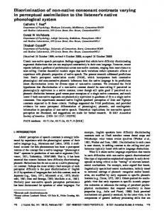
FIG. 3. Snapshots of the power flow P at times ct/b⫽0.6 and 1.2. Here, ⫹
⫹
(t)⫽e i ␣ ␦ (1) (t⫺i 2 T) as in Fig. 2, but with cT/b⫽1.2 共highly noncollimated PB兲 and ␣ ⫽ /3. 共a兲 and 共c兲: Distributions of P in the (z, ) plane 共all axes are normalized with respect to b兲. For clearer interpretation, the results are superimposed on the ellipsoidal wavefront corresponding to the coordinate system of Fig. 1. The arrows describe the size and direction of P. 共b兲 and 共d兲: snapshot of P z on the z axis at the same times.
⫹
⫹
关 共 ⫺1 兲 共 兲 /s 2 兴 / 关 共 兲 /cs 兴 ⬃O 关 cT/ 兩 z⫺ib 兩 兴 .
共3.4兲
In the far zone, the ratio on the right-hand side of 共3.4兲 is much smaller than unity. Under the collimation condition cTⰆb in 共2.26兲, this term is much smaller than unity also in the near zone 共i.e., along the entire z axis兲. Under these conditions, the terms containing (⫺1) in 共3.1兲 may be neglected for all z⬎0 so that 共3.3兲 becomes v⯝ 共 ⵜs r 兲 p/c⫺ 共 ⵜs i 兲¯p /c,
共3.5兲
where p is given by 共2.20兲 for points near the z axis. Note from 共2.16兲 with 共2.18兲 that near the z axis ⵜs r ⯝z˚ ⫹ /R(z)→z˚ and ⵜs i ⯝ /I(z)→0, where ⫽(x,y). Recall also that ⵜs r is orthogonal to the wavefronts whose local radius of curvature is R(z). In the far zone, we note from 共2.21兲 that ⵜs ⯝ⵜs r →r˚, hence 共3.6兲
v⯝r˚p/c, where here p is given in 共2.22兲. B. The power and energy flux
The power flux is defined as P共 r,t 兲 ⫽p 共 r,t 兲 v共 r,t 兲 .
共3.7兲
The expression obtained by inserting 共2.15兲 and 共3.3兲 is quite complicated. It is therefore convenient to explore the energy flux E共 r兲 ⫽ 1885
冕
⬁
⫺⬁
dt P共 r,t 兲 .
J. Acoust. Soc. Am., Vol. 107, No. 4, April 2000
共3.8兲
1
One finds that E共 r兲 ⫽ⵜs r 储 ␥ i 储 2 /c 兩 s 兩 2 ⫹ 具 ␥ i , ¯ 共␥⫺1 兲 典 共 s i ⵜs r ⫺s r ⵜs i 兲 / 兩 s 4 兩 , i 共3.9兲 ⬁ where 具 f ,g 典 ⫽ 兰 ⫺⬁ dt f (t)g(t) for any two real functions f and g. In deriving 共3.9兲 we used the following relations which apply for any real f and its Hilbert transform ¯f : 具 f , f 典 ⫽ 具¯f ,¯f 典 ⫽ 储 f 储 2 , 具 f ,¯f 典 ⫽ 具¯f , f 典 ⫽0, and 具 f , ˙f 典 ⫽0 共since f vanishes at t⫽⫾⬁). In the far zone, the second term in 共3.9兲 vanishes and the outward radiative energy is described only by the first term. Both terms are large in the near zone, in particular near B where s vanishes, and the field there dominated by strong reactive fields. The concept of time-dependent reactive field and energy has been introduced and analyzed in Ref. 39 in the context of electromagnetic fields. Using time-dependent spherical wave 共multipole兲 expansion, it has been shown that the time-dependent power radiated by an antenna consists of radiative and reactive pulses. The radiative power is a positive outgoing pulse and is unchanged as it propagates away from the source 共carries the same energy兲. The reactive power pulse, on the other hand, is strong in the near zone and vanishes in the far zone. It carries no net energy: at early times it propagates out and builds up a transient energy near the source, but after the radiative pulse has passed it discharges the energy back to the source region. This phenomenology is demonstrated in Fig. 3, which depicts snapshots of P. In order to be able to discern the off-axis properties of P and the low-frequency phenomena discussed in 共3.16兲 below, the PB parameters have been cho-
Heyman et al.: Physical source realization of pulsed beams
1885
⫹
sen to yield a highly noncollimated field. Specifically, (t) is the differentiated analytic ␦ used in Fig. 2, but with the PB parameter cT/b⫽1. Figure 3共a兲 and 共c兲 show the distribution of P in the (z, ) plane at times ct/b⫽0.6 and 1, while 3共b兲 and 共d兲 show plots of P z along the z axis at the same observation times. Note from Fig. 3共a兲 and 共c兲 that the flow lines in the near zone deviate from the normal to the wavefronts Es r 关see, e.g., 共3.9兲兴, and in particular the relatively strong ‘‘inward’’ flow near B. As discussed in 共3.16兲 below, this inward flow is strong near B, but the low-frequency components propagate inward also in front of the entire source disk E0 共see the shaded zones in Fig. 1兲. Indeed, in view of the ⫹
relatively low-frequency content of the signal chosen, the inward flow of reactive energy is readily observed as the negative part of P z behind the leading part of the signal in Fig. 3共d兲.
E rad共 s r 兲 ⫽
pˆ 共 r, 兲 ⫽ ˆ 共 兲 s ⫺1 e iks⫹i t ⬘ ⫽ ˆ 共 兲 s ⫺1 e i 共 ␥ r ⫹i ␥ i 兲 ,
共3.10a兲
vˆ共 r, 兲 ⫽ⵜs 关 c ⫺1 ⫺ 共 i s 兲 ⫺1 兴 pˆ 共 r, 兲 ,
共3.10b兲
where k⫽ /c and the carets denote field constituents with a suppressed time dependence e ⫺i t with ⬎0 共for ⬍0, one should take the complex conjugate of these expressions兲. Here ˆ ( ) is the 共rather arbitrary兲 spectrum of the pulse (t). In the high-frequency regime such that kbⰇ1, the solution in 共3.10兲 has the characteristics of a time-harmonic Gaussian beam 共see, e.g., Refs. 4–7 and 2兲 but we shall not dwell here on this interpretation. Using 共3.10兲 in conjunction with 共3.7兲 and 共3.8兲, we obtain E共 r兲 ⫽
1 Re
⫽
1 Re
冕 冕
⬁
0 ⬁
0
d pˆ 共 r, 兲 vˆ* 共 r, 兲 d 兩 ˆ 兩 2 兩 s 兩 ⫺2 e ⫺2 ␥ i 共 c ⫺1 ⫹ 共 i s * 兲 ⫺1 兲 ⵜs * , 共3.11兲
where the asterisks denote a complex conjugate. Next, we consider the total energy radiated out of the spheroidal wavefront Es r , E rad共 s r 兲 ⫽
冖
Es
E•dS,
共3.12兲
r
where dS is an area element on Es r . Substituting 共3.11兲, we note that on Es i we have ⵜs•dS⫽ 兩 ⵜs r 兩 dS, where 兩 ⵜs r 兩 is given in 共B2兲 and dS⫽h s i h ds i d , where the metric coefficients are given in 共B5兲. The -integration yields 2. Recalling that s i changes from ⫺b on the positive z axis to b on the negative axis, we end up with 1886
J. Acoust. Soc. Am., Vol. 107, No. 4, April 2000
⬁
d
b
⫺b
0
ds i E s r 共 s r ,s i , 兲
共3.13a兲
with E s r 共 s r ,s i , 兲 ⫽
冋
册
b 2 ⫹s r2 2 s i /k 兩 ˆ 兩 2 e ⫺2k 共 b⫹s i 兲 2 2 1⫹ 2 2 . bc s r ⫹s i s r ⫹s i
共3.13b兲 E s r is the spectral density of the ‘‘outward’’ 共i.e., the s r ) component of E. The s i integral in 共3.13兲 may readily be evaluated by rewriting 共3.13b兲 in the form E s r 共 s r ,s i , 兲 ⫽
冋
册
e ⫺2k 共 b⫹s i 兲 ⫺1 兩 ˆ 兩 2 共 b 2 ⫹s r2 兲 , b s i s r2 ⫹s 2i
共3.14兲
which provides a closed-form result for the outward flow between any two hyperbolas Hs i . Integrating over the full domain 共i.e., from s i ⫽⫺b to b兲, we end up with
C. Frequency-domain analysis of the energy flow
We shall explore the constituents discussed above in the frequency domain 共FD兲. The FD expressions corresponding to the field solutions in 共2.12兲 and 共3.1兲 are
冕 冕
E rad⫽
冕
⬁
0
d 兩 ˆ 兩 2
1⫺e ⫺4kb , b
共3.15兲
i.e., E rad⬎0 and is independent of s r as expected. Note that under the collimation condition in 共2.26兲, most of the signal energy is concentrated in the high-frequency range kbⰇ1 where the exponent in 共3.15兲 is negligible. While the total energy E rad flows outward, the local energy flux E s r may, in some regions, flow inward. From 共3.13b兲 the region Din( ) of inward energy flow is described by Din共 兲 :
s i /k s r2 ⫹s 2i
⬍⫺1.
共3.16兲
In general, Din( ) is located in front of E0 共where s i ⬍0). A detailed analysis of 共3.16兲 reveals that for frequencies such that kb⬎1, Din( ) has the shape of a ring in front of E0 whose boundary on E0 is given by ⫺k ⫺1 ⬍s i ⬍0 共see the dark-shaded region in Fig. 1兲. In particular, in the highcollimation range where kbⰇ1, this ring becomes concentrated near B. For low frequencies such that kb⬍1, on the other hand, Din( ) covers the entire front face of E0 共see the light-shaded region in Fig. 1兲. Recall though that at any given frequency, the total energy flows outward through Es r , as implied by 共3.15兲. It follows that at low frequencies, the energy is emitted by the back face of E0 : part of it flows around E0 and is absorbed by the front face, while the other radiates outward through Es r . The analysis above implies that for practical synthesis of the CSPB, the frequency spectrum of should be concentrated at frequencies such that kbⰇ1. Recalling that the effective width of the aperture in this range is W 0 ( )⫽ 冑b/k 关cf. 共2.25兲 and Ref. 2兴, it follows that for kb⬎2,W 0 is narrower than the inner radius of Din( ) which is given by s i ⫽⫺k ⫺1 关see 共3.16兲兴. Under these conditions the aperture can be truncated about the effective aperture W 0 of 共2.25兲, giving essentially the same field as the exact CSPB which is generated by the entire source disk E0 . Heyman et al.: Physical source realization of pulsed beams
1886
IV. SURFACE SOURCES AND EQUIVALENT SOURCES
B. Integral equations for alternative source realizations
We start by recalling the field discontinuity conditions implied by 共1.1兲. Let S be a given surface carrying surface sources ( s , f s ), i.e.,
⫽ s 共 rs ,t 兲 ␦ 共 n 兲 , f⫽n˚ f s 共 r,t 兲 ␦ 共 n 兲 ,
共4.1兲
where rs 苸S, n˚ is the normal to S at rS , pointing from side 1 to side 2 of S, and n is the coordinate along n˚. The field discontinuities implied by these sources are found from 共1.1兲 to be n˚• 共 v2 ⫺v1 兲 ⫽ s ,
p 2 ⫺p 1 ⫽n˚•fs ⬅ f s ,
共4.2兲
where (vi ,p i ) are the limiting value of (v, p) at side i of S. Next, let S be a closed surface that encloses all the sources to the field. We would like to synthesize the field outside S due to the sources inside S in terms of surface sources on it. As will be shown, there exist various realizations of these sources; of particular interest are those involving only or f sources. These alternative realizations are obtained by choosing inside S an arbitrary solution of the homogeneous field equation, denoted as (p in,vin). Using 共4.2兲, the surface sources are now given by
s ⫽n˚• 共 v⫺vin 兲 兩 S ,
f s ⫽ 共 p⫺ p in 兲 兩 S ,
1 ˚ 兴. p⫽ dS ⬘ 4 R 关关 ˙ s 兴 ⫹ 共 c ⫺1 关 ˙f s 兴 ⫹R ⫺1 关 f s 兴 兲 n˚⬘ •R S 共4.4兲
This integral synthesizes the true field (p,v) at points outside S and the arbitrarily chosen field (p in,vin) at points inside S. A. Kirchhoff realization
As mentioned before, different source realizations are generated by choosing different homogeneous solutions (p in,vin) in 共4.3兲. One such choice, p in⫽0,
vin⫽0,
共4.5兲
gives rise to what will be identified below as the Kirchhoff realization. Using 共4.5兲 and 共4.3兲, the Kirchhoff sources are
s ⫽n˚•v兩 S ⫽⫺ n ⫺1 t p兩S ,
f s ⫽p 兩 S ,
共4.6兲
where in the second expression for s we used 共1.1b兲 to replace the limiting value of v outside S by the value of p there. When the sources in 共4.6兲 are substituted into 共4.4兲, we obtain the true field outside S and a null contribution inside S. Using 共4.6兲 in 共4.4兲, one obtains the conventional Kirchhoff integral representation for the radiating field in terms of the values of p and n p on S, which is usually obtained by using the scalar wave equation for p in conjunction with Green’s theorem.40 Thus, Eq. 共4.6兲 provides the surface source realization of this formula. 1887
J. Acoust. Soc. Am., Vol. 107, No. 4, April 2000
pf⫽
冕
S
1 ˚, dS ⬘ 4 R 共 c ⫺1 关 p˙ 兴 ⫹R ⫺1 关 p 兴 兲 n˚⬘ •R 共4.7兲
冕
⫺1 p ⫽ dS ⬘ 关 p兴. 4 R n⬘ S
The s -only realization involves the s sources in 共4.6兲 plus an additional term denoted as sf that gives rise to the known field p f outside S. sf is therefore calculated via the integral equation on S
共4.3兲
where n˚ is an outward normal to S. Substituting 共4.3兲 into 共1.2兲, we obtain
冕
Equation 共4.4兲 synthesizes the field outside S due to the sources inside S in terms of both s and f s sources. Alternative formulations are obtained if one chooses different values for (p in,vin). We shall look, in particular, for realizations such that either f s or s in 共4.3兲 vanishes identically on S. These sources are determined via an integral equation as described below. We start by expressing the field 共4.4兲 for the special case of the sources in 共4.6兲 as a sum of two terms: p⫽p ⫹p f denoting, respectively, the fields due to the f s and s sources in 共4.6兲. Substituting 共4.6兲 in 共4.4兲, these fields may be expressed in terms of the known field p outside S
冕
S
dS ⬘
1 关 ˙ f 兴 ⫽ p f 共 r,t 兲 , 4R s
r,r⬘ 苸S,
共4.8兲
where p f is given in 共4.7兲 in terms of the known field p on the outer side of S. Note that the kernel on the left-hand side of 共4.8兲 is singular at r⬘ ⫽r, but this singularity can be extracted explicitly using principal value integration. The solution of 共4.8兲 is not unique. Recalling from 共4.3兲 that the internal field (p in,vin) in the s -only realization satisfies p in兩 S ⫽ p 兩 S where p is the known pressure field outside S, it follows that the null space of 共4.8兲 is described by internal field solutions that satisfy p in兩 S ⫽0. Such solutions are possible at discrete frequencies n , n⫽1,2,..., which are the internal resonance frequencies of S for the ‘‘soft’’ boundary condition p in兩 S ⫽0. The solution of 共4.8兲 can therefore be augmented by a discrete set of eigensolutions of the form sf (r,t)⫽ 兺 n Re an sn(r)e ⫺i n t , which do not affect the field outside S. A unique solution is obtained by imposing another criterion, say a minimum energy condition. We shall not consider this subject here. Similarly, the f s -only realization involves the f s sources of 共4.6兲 plus an additional term f s that generates the p field outside S. f s is found via the integral equation on S
冕
S
dS ⬘
1 ˚ ⫽p 共 r,t 兲 , 共 c ⫺1 关 ˙f s 兴 ⫹R ⫺1 关 f s 兴 兲 n˚⬘ •R 4R
r,r⬘ 苸S, 共4.9兲
where p is given in 共4.7兲 in terms of the known field p on the outer side of S. As discussed after 共4.8兲, the solution of 共4.9兲 is not unique: its null space is described by the internal resonance frequencies associated the ‘‘hard’’ boundary condition n p in兩 S ⫽0. Heyman et al.: Physical source realization of pulsed beams
1887
FIG. 4. Waveforms of the surface sources in 共5.1兲 on S⫽Es r with s r ⫽0.1b. The waveforms are depicted in the (ct,s i ) plane with s i , the coordinate along Es r varies from ⫺b on the positive z axis to b on the negative axis. 共a兲 and 共b兲: 1 s ; 共c兲 and 共d兲: 2 s ; ⫹
共e兲 and 共f兲: f s . The pulse is the differentiated analytic ␦ used in Fig. 2 with high-collimation parameter cT/b ⫽10⫺3 .
V. SOURCE DISTRIBUTIONS FOR THE CSPB
It is convenient to consider a source realization on the ellipsoid Es r of 共2.9兲 for a given s r ⬎0. Substituting 共2.12兲 and 共3.1兲 into 共4.6兲, we obtain ⫹
⫹
s ⫽ 兩 ⵜs r 兩 Re兵 共 兲 /cs⫹ 共 ⫺1 兲 共 兲 /s 2 其 , ⫹
f s ⫽Re兵 共 兲 /s 其 ,
共5.1a兲 共5.1b兲
where s, , and 兩 ⵜs r 兩 are given in 共2.5b兲, 共2.12兲, and 共B2兲, respectively. These expressions are functions of s i , which serves as a coordinate along Es r . 1888
J. Acoust. Soc. Am., Vol. 107, No. 4, April 2000
Explicit expressions are obtained for the special case when Es r shrinks to the source disk E0 of 共2.7兲. Denoting values on the front and back faces of E0 by the superscript ⫾, respectively, we find that s ⫾ ⫽⫿i ,
␥ ⫾ ⫽i 共 b⫿ 兲 /c,
where ⫽ 冑b 2 ⫺ 2 . 共5.2兲
Substituting 共2.12兲 and 共3.1兲 into 共4.6兲, we obtain ⫹ ⫹ b s⫾ ⫽ Re兵 ⫾i 关 t⫺i 共 b⫿ 兲兴 / c⫺ 共 ⫺1 兲 关 t⫺i 共 b⫿ 兲兴 / 2 其 ,
共5.3a兲
Heyman et al.: Physical source realization of pulsed beams
1888
FIG. 5. Same as Fig. 4, but for noncollimated source with cT/b⫽1. ⫹
f z⫾ ⫽⫾p 兩 E⫾ ⫽Re兵 i 关 t⫺i 共 b⫿ 兲兴 / 其 , s
共5.3b兲
0
where the upper and lower signs correspond to sources on the front and back face of E0 , respectively, while f z⫾ in the s last expression denotes the z component of the fs source on the front and back faces of E0 . Note also the algebraic singularity of the sources at ⫽b on the circle B. Special attention should be given to the collimated case 共2.26兲 which is the most important one for practical applications. We note that in this case the relevant part of the source is concentrated within the effective aperture W 0 共2.25兲 on the front face of E0 , which is much narrower than the entire disk E0 关see 共2.27兲兴. Furthermore, under the collimation condition the contribution of the second term in s is negligible 关see the discussion in 共3.4兲兴. Finally, from 共5.2兲 it follows that for ⫺ ⫹ 2 Ⰶb, ␥ ⫹ i ⬇ /2cb, while ␥ i ⬇2ib/c, hence in 共5.3兲 s ⫺ ⫹ ⫺ Ⰷ s and f z Ⰷ f z . Thus, Eq. 共5.3兲 reduces to the simplified s s explicit expression for effective sources ⫹
c s ⫽ f z s ⫽b ⫺1 Re兵 i 共 t⫺i 2 /2cb 兲 其 , 1889
⬃O 共 W 0 兲 .
J. Acoust. Soc. Am., Vol. 107, No. 4, April 2000
共5.4兲
These simplified sources generate a strong PB field along the positive z axis that behaves paraxially like the PB in 共2.17兲 关or 共2.20兲兴. In all other directions, the resulting field is weak but due to the approximation in 共5.4兲 it does not have the exact known form of 共2.12兲. Alternatively, one may use only the s or the f s sources in 共5.4兲. This generates collimated PB along both the positive and the negative z directions: From 共4.4兲, the s source radiates symmetrically in both directions while the f s source radiates antisymmetrically. Taken together, the contributions of s and of f s enhance each other in the positive direction and cancel each other in the negative direction, thereby radiating a strong PB field only along the positive z axis and a weak field elsewhere. Figures 4 and 5 depict the surface sources of the CSPB realized on an ellipsoidal wavefront S⫽Es r as in 共5.1兲. Here, s r is taken to be 0.1b so that Es r is close to the branch disk E0 共see Fig. 1兲. The waveforms are depicted in the (ct,s i ) plane with s i being a coordinate along Es r (s i varies from ⫺b on the positive z axis to b on the negative axis兲. The first and Heyman et al.: Physical source realization of pulsed beams
1889
second terms in 共5.1a兲 are termed 1 s and 2 s , respectively.
given real signal (t), t苸R, with frequency spectrum
The pulse is the differentiated analytic ␦ used in Figs. 2 and 3. In Fig. 4 we use a short pulse with cT/b⫽10⫺3 which yields a collimated PB, while in Fig. 5 cT/b⫽1, yielding a noncollimated field. Note that the effective width of the source distribution in Fig. 4 agrees with the estimates for W 0 in 共2.25兲; hence, the sources there can be truncated and described by the simpler expressions in 共5.4兲. In Fig. 5, on the other hand, the source distribution is much wider. In this case one also observes the relatively strong sources at points near B(s i ⯝0), which are insignificantly small under the collimation condition in Fig. 4. These sources become stronger for smaller s r , and become singular when S shrinks to the branch disk E0 , yet their contribution is insignificant in the collimation condition.
ˆ ( ), the dual analytic signal ( ) is defined via the onesided inverse Fourier transform
⫹
⫹
⫹ 1 共 兲⫽
冕
⬁
0
d e ⫺i ˆ 共 兲 ,
Im ⭐0.
共A1兲
⫹
It follows that ( ) is an analytic function in the lower half of the complex plane. This function may also be defined directly from the real data (t) for real t via
共 兲⫽
1 i
冕
⬁
⫺⬁
dt
共 t 兲 , ⫺t
Im ⭐0.
共A2兲
From 共A2兲, the limit of on the real t axis is related to the real signal 共兲 via ⫹
共 t 兲 ⫽ 共 t 兲 ⫹i ¯ 共 t 兲 ,
VI. SUMMARY AND CONCLUSIONS
Our aim in the present paper has been to explore this physical source realization of the CSPB. This has been done within the framework of the acoustic field, by deriving expressions for the acoustic source distributions and by exploring the power and energy flux near these sources. The surface sources have been derived via the field equivalence theorems in Sec. IV. The exact source solutions derived in 共5.1兲 关or 共5.3兲兴 generate the globally exact CSPB. Yet, from a practical point of view special emphasis has been given to the parameter range cTⰆb 关see 共2.26兲兴; T is the pulse length and b is the collimation distance兲 where the CSPB is well collimated: in this special case the CSPB can be realized effectively by the simple truncated source distribution in 共5.4兲 whose spatial support W 0 of 共2.25兲 is much smaller than the source support of the exact CSPB. In order to further clarify the properties of source realization, we have also explored the power flux near the sources. It has been shown 关see 共3.16兲兴 that at high frequencies such that kbⰇ1 共k is the wave number兲 the energy is emitted by a narrow aperture on the front face of the source disk E0 . At low frequencies, on the other hand, the energy is emitted by the back face of E0 : part of it flows around E0 and is absorbed by the front face, while the rest radiates outward through Es r . Thus, for practical synthesis the frequency spectrum of the CSPB should be concentrated in the highfrequency regime, which supports the conclusions of the preceding paragraph. ACKNOWLEDGMENTS
This work is supported in part by the U.S. Air Force Office of Scientific Research under Grant No. F49620-98-C0013, managed by The Virginia Center for Signals and Waves, and in part by the Israel Science Foundation under Grant No. 404/98. APPENDIX A: ANALYTIC SIGNALS
In order to deal with the complex propagation delays implied by the complex sources, one needs to use analytic signals that can accommodate complex time variables. For a 1890
J. Acoust. Soc. Am., Vol. 107, No. 4, April 2000
共A3兲
t real,
where ¯ 共 t 兲 ⫽
⫺1
冕
⬁
⫺⬁
dt ⬘ P
共 t⬘兲 t⫺t ⬘
is the Hilbert transform, with P denoting Cauchy’s principal value. The real signal for real t can therefore be recovered ⫹
via (t)⫽Re (t). ⫹
Thus, if p (r,t) is an analytic solution of the time⫹
⫹
dependent wave equation, then both p r ⫽Re p and p i ⫽Im p are real solutions of the wave equation. Henceforth, we shall only consider p r since p i or any other linear combination of ⫹
p r and p i can be obtained by multiplying p by a complex constant and then taking the real part. APPENDIX B: ADDITIONAL PROPERTIES OF THE OS SYSTEM
From 共2.8兲, one may readily infer the following relations: s r2 ⫺s 2i ⫽r 2 ⫺b 2 , s r s i ⫽⫺zb,
共B1兲
ⵜs r ⫽ 共 rs r ⫺bs i 兲 / 兩 s 兩 2 , 兩 ⵜs r 兩 ⫽ 冑b 2 ⫹s r2 / 兩 s 兩 ,
共B2兲
ⵜs i ⫽⫺ 共 rs i ⫹bs r 兲 / 兩 s 兩 2 , 兩 ⵜs i 兩 ⫽ 冑b 2 ⫺s 2i 兩 s 兩 ,
共B3兲
ⵜs r •ⵜs i ⫽0,
共B4兲
and the metric coefficients40 along the (s r ,s i , ) coordinates are h s r ⫽ 兩 s 兩 / 冑b 2 ⫹s r2 ,
h s i ⫽ 兩 s 兩 / 冑b 2 ⫺s 2i ,
h ⫽b ⫺ 冑b 2 ⫹s r2 冑b 2 ⫺s 2i .
共B5兲
1
E. Heyman and B. Z. Steinberg, ‘‘A spectral analysis of complex source pulsed beams,’’ J. Opt. Soc. Am. A 4, 473–480 共1987兲. 2 E. Heyman and L. B. Felsen, ‘‘Complex source pulsed beam fields,’’ J. Opt. Soc. Am. A 6, 806–817 共1989兲. 3 E. Heyman, B. Z. Steinberg, and R. Ianconescu, ‘‘Electromagnetic complex source pulsed beam fields,’’ IEEE Trans. Antennas Propag. AP-38, 957–963 共1990兲. 4 G. A. Deschamps, ‘‘Gaussian beams as a bundle of complex rays,’’ Electron. Lett. 7, 684–685 共1971兲. Heyman et al.: Physical source realization of pulsed beams
1890
5
J. W. Ra, H. Bertoni, and L. B. Felsen, ‘‘Reflection and transmission of beams at dielectric interfaces,’’ SIAM 共Soc. Ind. Appl. Math.兲 J. Appl. Math. 24, 396–412 共1973兲. 6 L. B. Felsen, ‘‘Complex-source-point solutions of the field equations and their relation to the propagation and scattering of Gaussian beams,’’ in Symposia Matematica, Istituto Nazionale di Alta Matematica 共Academic, London, 1976兲, Vol. XVIII, pp. 40–56. 7 S. Y. Shin and L. B. Felsen, ‘‘Gaussian beam modes by multipoles with complex source points,’’ J. Opt. Soc. Am. 67, 699–700 共1977兲. 8 G. Kaiser, A Friendly Guide to Wavelets 共Birkhauser, Boston, 1994兲, pp. 276–279. 9 E. Heyman, R. Strachielevitz, and D. Koslof, ‘‘Pulsed beam reflection and transmission at a planar interface: Exact solutions and approximate local models,’’ Wave Motion 18, 315–343 共1993兲. 10 R. Ianconescu and E. Heyman, ‘‘Pulsed beam diffraction by a perfectly conducting wedge. I. Exact solution,’’ IEEE Trans. Antennas Propag. AP42, 1377–1385 共1994兲. 11 E. Heyman and R. Ianconescu, ‘‘Pulsed beam diffraction by a perfectly conducting wedge. Part II: Local scattering models,’’ IEEE Trans. Antennas Propag. AP-43, 519–528 共1995兲. 12 E. Heyman, ‘‘Pulsed beam propagation in an inhomogeneous medium,’’ IEEE Trans. Antennas Propag. AP-42, 311–319 共1994兲. 13 A. N. Norris, B. S. White, and J. R. Schrieffer, ‘‘Gaussian wave packets in inhomogeneous media with curved interfaces,’’ Proc. R. Soc. London, Ser. A 412, 93–123 共1987兲. 14 E. Heyman, A. G. Tijhuis, and J. Boersma, ‘‘Spherical and collimated pulsed fields in conducting media,’’ Proceedings of URSI Trianum International Symposium on Electromagnetic Theory, St. Petersburg, 1995, pp. 643–645 共unpublished兲. 15 T. Melamed and L. B. Felsen, ‘‘Pulsed beam propagation in lossless dispersive media. I. Theory,’’ J. Opt. Soc. Am. A 15, 1268–1276 共1998兲. 16 T. Melamed and L. B. Felsen, ‘‘Pulsed beam propagation in lossless dispersive media. Part II. Applications,’’ J. Opt. Soc. Am. A 15, 1277–1284 共1998兲. 17 J. Oz and E. Heyman, ‘‘Modal theory for the two-frequency mutual coherence function in random media. Beam waves,’’ Waves Random Media 8, 159–174 共1998兲. 18 J. Gozani, ‘‘Pulsed beam propagation through random media,’’ Opt. Lett. 21, 1712–1714 共1996兲. 19 S. Zeroug, F. E. Stanke, and R. Burridge, ‘‘A complex-transducer-point model for finite emitting and receiving ultrasonic transducers’’ Wave Motion 24, 21–40 共1996兲. 20 S. Feng and H. G. Winful, ‘‘Spatiotemporal transformations of isodiffracting ultrashort pulses by nondispersive quadratic phase media,’’ J. Opt. Soc. Am. A 16, 2500–2509 共1999兲. 21 M. A. Porras, ‘‘Ultrashort pulsed Gaussian light beams,’’ Phys. Rev. E 58, 1086–1093 共1998兲. 22 M. A. Porras, ‘‘Nonsinusoidal few-cycle pulsed light beams in free space,’’ J. Opt. Soc. Am. B 16, 1468–1474 共1999兲. 23 E. Heyman, ‘‘Complex source pulsed beam expansion of transient radiation,’’ Wave Motion 11, 337–349 共1989兲.
1891
J. Acoust. Soc. Am., Vol. 107, No. 4, April 2000
24
B. Z. Steinberg, E. Heyman, and L. B. Felsen, ‘‘Phase space beam summation for time dependent radiation from large apertures: Continuous parametrization,’’ J. Opt. Soc. Am. A 8, 943–958 共1991兲. 25 B. Z. Steinberg and E. Heyman, ‘‘Phase space beam summation for time dependent radiation from large apertures: Discretized parametrization,’’ J. Opt. Soc. Am. A 8, 959–966 共1991兲. 26 T. Melamed, ‘‘Phase space beam summation: A local spectrum analysis of time dependent radiation,’’ J. Electromagn. Waves Appl. 11, 739–773 共1997兲. 27 E. Heyman and I. Beracha, ‘‘Complex multipole pulsed beams and Hermite pulsed beams: A novel expansion scheme for transient radiation from well collimated apertures,’’ J. Opt. Soc. Am. A 9, 1779–1793 共1992兲. 28 T. B. Hansen and A. N. Norris, ‘‘Exact complex source representations of transient radiation,’’ Wave Motion 26, 101–115 共1997兲. 29 T. Melamed, E. Heyman, and L. B. Felsen, ‘‘Local spectral analysis of short-pulse-excited scattering from weakly inhomogeneous media. I. Forward scattering,’’ IEEE Trans. Antennas Propag. AP-47, 1208–1217 共1999兲. 30 T. Melamed, E. Heyman, and L. B. Felsen, ‘‘Local spectral analysis of short-pulse-excited scattering from weakly inhomogeneous media. II. Inverse scattering,’’ IEEE Trans. Antennas Propag. AP-47, 1218–1227 共1999兲. 31 J. N. Brittingham, ‘‘Focus wave modes in homogeneous Maxwell’s equations: Transverse electric mode,’’ J. Appl. Phys. 54, 1179–1189 共1983兲. 32 R. W. Ziolkowski, ‘‘Exact solutions of the wave equation with complex source locations,’’ J. Math. Phys. 26, 861–863 共1985兲. 33 A. M. Shaarawi, I. M. Besieris, R. W. Ziolkowski, and S. M. Sedky, ‘‘The generation of approximate focus wave mode pulses from wide-band dynamic Gaussian apertures,’’ J. Opt. Soc. Am. A 12, 1954–1964 共1995兲. 34 E. Heyman, ‘‘The focus wave mode: A dilemma with causality,’’ IEEE Trans. Antennas Propag. AP-37, 1604–1608 共1989兲. 35 J. Durnin, J. J. Miceli, Jr., and J. H. Eberly, ‘‘Diffraction free beam’’ Phys. Rev. Lett. 58, 1499–1452 共1987兲. 36 J.-y. Lu and J. F. Greenleaf, ‘‘Nondiffracting X waves—exact solutions to free space scalar wave equation and their finite aperture realizations,’’ IEEE Trans. Ultrason. Ferroelectr. Freq. Control 39, 19–31 共1992兲. 37 H. E. Moses and R. T. Prosser, ‘‘Initial conditions, sources, and currents for prescribed time-dependent acoustic and electromagnetic fields in three dimensions. I. The inverse initial value problem. Acoustic and electromagnetic ‘‘bullets,’’ expanding waves, and imploding waves,’’ IEEE Trans. Antennas Propag. AP-34, 188–196 共1986兲. 38 H. E. Moses and R. T. Prosser, ‘‘Acoustic and electromagnetic bullets. New exact solutions of the acoustic and Maxwell’s equation,’’ SIAM 共Soc. Ind. Appl. Math.兲 J. Appl. Math. 50, 1325–1340 共1990兲. 39 A. Shlivinski and E. Heyman, ‘‘Time domain near field analysis of short pulse antennas. Part I: Spherical wave 共multipole兲 expansion;’’ ‘‘Part II Reactive energy and the antenna Q,’’ IEEE Trans. Antennas Propag. AP47, 271–279 共1999兲; AP-47, 280–286 共1999兲. 40 J. A. Stratton, Electromagnetic Theory 共McGraw-Hill, New York, 1941兲.
Heyman et al.: Physical source realization of pulsed beams
1891