Using JASA format

Optimum near-field performance of microphone arrays subject to a far-field beampattern constraint James G. Ryana) Acoustics and Signal Processing, Institute for Microstructural Sciences, National Research Council Canada, Ottawa, Ontario K1A 0R6, Canada

Rafik A. Goubran Systems and Computer Engineering, Carleton University, Ottawa, Ontario K1S 5B6, Canada

共Received 8 September 1999; revised 15 August 2000; accepted 15 August 2000兲 This article addresses the problem of maximizing the near-field gain of a microphone array subject to a constraint on the far-field beampattern. The problem arises when acquiring speech from a near-field talker in the presence of a strong source of interference located farther from the array. When the angles of incidence from the near-field target and the far-field interference are identical, enforcing a null constraint in the interference direction reduces array gain and robustness. This article shows how to mitigate this effect by selection of the constrained response level. A suitable selection is to force the beampattern in the interference direction to be proportional to the unconstrained beampattern. The proportionality constant can then be used to trade off interference reduction and array gain. Specific numerical examples are provided. © 2000 Acoustical Society of America. 关S0001-4966共00兲04711-1兴 PACS numbers: 43.60.Gk, 43.38.Hz 关JCB兴

I. INTRODUCTION

This article addresses the problem of maximizing the near-field gain of a microphone array subject to a constraint on the far-field response pattern. It specifically deals with situations where the near-field signal source and the far-field interference are located along the same angle of incidence with respect to the array axis and both are immersed in a spherically isotropic noise field. This arises in speech pickup in rooms, for example, when a strong wall reflection or noise source originates from a location behind the near-field talker. The direct wave from both target and interference arrive at the array with the same angle of incidence; however, the interfering wavefront possesses a larger radius of curvature due to the increased distance between the source and the array. Currently available methods simplify the analysis and design of microphone arrays by assuming that all acoustic sources are located far from the array. In such cases wavefront curvature observed at the array position is very small and all waves impinging upon the array are assumed to be planar. There are circumstances, however, where the signal source is located very close to the array and the assumption of plane wave propagation is not valid.1 This situation arises, for instance, in the application of microphone arrays to mobile telephony2,3 and conference telephony in small rooms.4,5 In these cases, the talker is located in the array’s near field and wavefront curvature can be detected within the array’s aperture. Beamformer synthesis methods that explicitly include target wavefront curvature have recently been investigated. a兲

Present address: Communications Research Center, 3701 Carling Ave., Ottawa, Ontario K2H 8S2, Canada.

2248

J. Acoust. Soc. Am. 108 (5), Pt. 1, Nov 2000

Current approaches provide a beamformer either with a desired spatial response pattern6–8 or with an optimal response based on a suitable figure of merit.2,9 The problem of imposing a beampattern constraint on an optimized array has been addressed only in the case of farfield targets. Optimization approaches considered include maximizing array gain,10,11 maximizing signal-to-noise ratio 共SNR兲,12 minimizing the sensor weight-vector norm,13,14 and minimizing the beampattern disturbance caused by the added constraint.15,16 Since all of these problem formulations involve the optimization of a quadratic performance index subject to a linear constraint, the solutions are related under the appropriate conditions.13,17,16 Steyskal18 has addressed a mixed near-field/far-field problem which arises in the design of antenna systems. The objective was to minimize the effects of a near-field scatterer on the radiated beampattern of a phased array antenna. Using an extension of the method in Ref. 16 it was shown that a near-field response null can be imposed with minimal impact on the far-field beampattern. The idea proposed in this work is essentially the opposite of Steyskal’s, that is, to impose a far-field null while maintaining the response to a near-field target. The main difference is that the optimization goal is maximizing the near-field array gain rather than minimizing the pattern disturbance. Consequently, the objective is similar to that in Refs. 10 and 11; however, the derivation uses the results from linearly constrained minimum variance 共LCMV兲 beamforming19 and incorporates the concept of generalized angle found in Ref. 20. Furthermore, the result is generalized to include an arbitrary response level in the interference direction rather than a null. As is shown, proper selection of the constrained response level can reduce the impact of the constraint on the overall array performance. This article is organized as follows. Concepts of conven-

0001-4966/2000/108(5)/2248/8/$17.00

© 2000 Acoustical Society of America

2248

tional array optimization methods are first outlined. Both unconstrained as well as linearly constrained optimization are reviewed. Next, the sensor weight vector and array gain are derived for the specific case of dual linear constraints: one representing the signal direction and another representing the interference or noise direction. The derivation generalizes that found in Refs. 10 and 11 by including an arbitrary response level at the interference location 共as opposed to forcing a zero response兲. The generalized array-gain expression is then used to derive a noise-response target that permits a controlled trade-off of array gain. The results are illustrated using the specific example of a uniformly spaced linear array.

Array gain G is defined as the ratio of output SNR over the SNR observed at a single sensor. For an M-element array, it is given by WH Rss W , WH Rnn W

共1兲

where W is the M ⫻1 vector of complex sensor weights WT ⫽ 关 W 0

W1

¯

W M ⫺1 兴 ,

共2兲

and Rss and Rnn are the M ⫻M signal and noise correlation matrices defined as Rss ⫽E 兵 S•SH 其

⫺1 S. G opt⫽SH Rnn

共5兲

For certain noise correlation matrices, the unconstrained optimum weight solution Eq. 共4兲 can lead to a beamformer that is intolerant of sensor noise and other types of random errors. Improved robustness can be obtained, however, by including a small diagonal term in the definition of Rnn . That is, define Rnn ⫽Q⫹ ␦ 2 I,

II. REVIEW OF UNCONSTRAINED AND LINEARLY CONSTRAINED ARRAY-GAIN MAXIMIZATION

G⫽

is only unique to within a constant scale factor. Thus, the array gain is insensitive to a scaling of the weights. This added degree of freedom in selecting Wopt can be used to control the amplitude of the array output or to provide a flat frequency response for a broadband beamformer. The maximum array gain G opt is

共3兲

and

共6兲

where Q is the correlation matrix of the environmental noise, I is an M ⫻M identity matrix, and ␦ 2 is a small positive constant used to control beamformer robustness. This modification allows simple, unconstrained optimization to be used to design a beamformer with an effective constraint on robustness. This array optimization approach has been used to enhance the far-field performance of microphone arrays in noisy and reverberant environments.23–25 Fixed, optimum arrays were designed based on an isotropic model of the interfering field and a plane wave model for the target. Results obtained with these optimized arrays demonstrate enhanced reception of speech signals in realistic situations. The extension of this concept to near-field targets is capable of providing a further increase in array gain.9

Rnn ⫽E 兵 N•NH 其 with S being the signal propagation vector and N the noise propagation vector. The superscripts T and H denote matrix transpose and conjugate transpose, respectively. The complex microphone weights defined in Eq. 共2兲 apply to a specific frequency. Since speech signals are broadband, a practical implementation of these weights must be performed in the frequency domain 关using a fast Fourier transform 共FFT兲兴 or by designing a finite impulse response 共FIR兲 filter that provides the correct amplitude and phase at frequencies within the band of interest.

Provided that Rnn is nonsingular, the value of the quotient Eq. 共1兲 is bounded by the minimum and maximum ei⫺1 Rss . The array gain genvalues of the symmetric matrix Rnn is maximized by setting the weight vector W equal to the eigenvector corresponding to the maximum eigenvalue.21 In the special case where Rss is a dyad defined by the outer product Rss ⫽SSH , then the weight vector Wopt that maximizes G is given simply by22 共4兲

where ␹ is an arbitrary complex constant. Inclusion of the complex constant ␹ implies that the optimum weight vector 2249

J. Acoust. Soc. Am., Vol. 108, No. 5, Pt. 1, Nov 2000

To exert control over the array beampattern while optimizing performance, it is necessary to employ linear constraints. While various types of linear constraints are possible, this article focuses on the use of point constraints to constrain the response at a specific locations. Nonetheless, derivative and eigenvector constraints can also be used to exert broader control over the response shape.19 A single, linear constraint is expressed as 共7兲

cH W⫽g,

A. Unconstrained gain maximization

⫺1 Wopt⫽ ␹ Rnn S,

B. Linearly constrained gain maximization

where c is an M ⫻1 constraint vector and g is the desired response level. Point-constraint vectors correspond to the signal propagation vectors associated with the spatial constraint locations. For example, to constrain a linear array’s far-field beampattern at an angle ␪ the following point constraint is required: cT ⫽ 关 e jkx 0 cos ␪ e jkx 1 cos ␪ ¯

e jkx M ⫺1 cos ␪ 兴 ,

where x m are the positions of the microphones and k is the wave number. Multiple constraints can be enforced by defining a constraint matrix C, whose L columns consist of individual constraint vectors c, and a vector g of the corresponding responses g. The multiple constraint equation is CH W⫽g. J. G. Ryan and R. A. Goubran: Optimum near-field performance

2249

The constrained optimization problem is then posed as H

maximize G, subject to C W⫽g. The method of Lagrange multipliers can be used to transform this constrained optimization problem into an unconstrained one. The problem is simplified by restating the gain maximization goal in an equivalent form. That is, maximizing array gain is equivalent to minimizing the noise response, as represented by the denominator of Eq. 共1兲, with a constraint on the signal response, as represented by the numerator of Eq. 共1兲. The signal response constraint can be handled easily as one of the columns in C. The optimization problem then becomes

strated for a near field S and a far field N; however, the results apply equally well to S and N in the near field or far field.

A. Optimum weights

Define the M ⫻2 constraint matrix as C⫽ 关 S

where S and N represent assumed signal and noise vectors, respectively. The 2⫻1 gain vector is g⫽

minimize WH Rnn W⫹␭H 共 CH W⫺g兲 ⫹␭T 共 CH W⫺g兲 , where ␭ is the Lagrange multiplier vector. The weight vector that solves this problem is given by the well-known solution19 ⫺1 ⫺1 Wopt⫽Rnn C关 CH Rnn C兴 ⫺1 g.

共8兲

Under equivalent conditions, the constrained optimum solution of Eq. 共8兲 yields the same solution as the unconstrained solution Eq. 共4兲. To see this, consider the case of a single point constraint at the signal location C⫽S. The constraint equation is SH W⫽g s ,

共9兲

which is equal to the unconstrained solution given in Eq. 共4兲 with

␹⫽

gs ⫺1 SH Rnn S

冋册

gs . gn

The effect of this constraint system is to force the beamformer to have a response of g s at a location corresponding to vector S and a response of g n at a location corresponding to vector N. The value of g s is chosen to provide a desired signal level at the array output and the value of g n is chosen to suppress the interference. In principle, the values of both these parameters can be set arbitrarily; however, the choice of g n has an impact on overall beamformer performance, as will be discussed later. Substituting the constraints into the expression for the optimum weights Eq. 共8兲 yields

where g s is the desired signal level. According to Eq. 共8兲 the linearly constrained optimum weights are ⫺1 S Rnn Wopt⫽ H ⫺1 g s , S Rnn S

N兴 ,

⫺1 S Wopt⫽ 关 Rnn

⫺1 Rnn N兴

冋

⫺1 SH Rnn S H

N

⫺1 Rnn S

⫺1 SH Rnn N

N

H

⫺1 Rnn N

册冋册 ⫺1

gs . gn

The inverse of the 2⫻2 matrix can be written as

冋

⫺1 SH Rnn S

⫺1 SH Rnn N

⫺1 NH Rnn S

⫺1 NH Rnn N

⫽

冋

册

⫺1

册

⫺1 ⫺1 NH Rnn N ⫺SH Rnn N 1 , • ⫺1 ⫺1 H H D ⫺N Rnn S S Rnn S

confirming that the two optimization approaches yield equivalent results.

where D is the matrix determinant

III. NEAR-FIELD GAIN MAXIMIZATION SUBJECT TO A FAR-FIELD BEAMPATTERN CONSTRAINT

Substituting the expression for the inverse matrix, multiplying through, and rearranging terms yields the following solution for the optimum weights

This article examines the impact of a single, linear constraint on the performance of an optimized array. The derivation presented herein allows the specification of an arbitrary response level. As discussed earlier, however, the optimum array weights are insensitive to scaling by a constant factor. Without further precautions, the solution to the constrained optimization problem would be to simply scale the entire unconstrained beampattern. Both the target and interference would be scaled by the same amount. To avoid this situation, this derivation includes two linear constraints. One constraint is used to control the beamformer response in the target direction S while the other is used to control the response in a known interference direction N. The only assumption made about S and N is that they are not identical ⫺1 C would not be 共otherwise the matrix represented by CH Rnn invertible兲. In the following material, results will be demon2250


⫺1 ⫺1 ⫺1 D⫽ 关 SH Rnn S兴关 NH Rnn N兴 ⫺ 兩 SH Rnn N兩 2 .

Wopt⫽

1 1⫺ 共 cos ␥ 兲 2 • 关 g s Ws ⫺g n Ws SH Wn ⫹g n Wn ⫺g s Wn NH Ws 兴 .

共10兲

In this expression, Ws is the unconstrained optimum weight vector for a source located at S 关see Eq. 共9兲兴, Ws ⫽

⫺1 S Rnn ⫺1 SH Rnn S

,

Wn is the unconstrained optimum weight vector for a source located at N, Wn ⫽

⫺1 Rnn N ⫺1 NH Rnn N

,

J. G. Ryan and R. A. Goubran: Optimum near-field performance

2250

and (cos ␥)2 is the cosine squared of the generalized angle ␥ between the constraint vectors S and N defined as20 共 cos ␥ 兲 2 ⫽

⫺1 兩 SH Rnn N兩 2 ⫺1 ⫺1 SH Rnn S•NH Rnn N

共11兲

.

vectors S and N are orthogonal, then (cos ␥)2⫽0 and the denominator term has no effect. As (cos ␥)2→1, however, the denominator approaches 0 and the weight magnitudes increase drastically. Under this condition, the resulting array has very low robustness.

Note that, due to the Schwarz inequality, 0⭐ 共 cos ␥ 兲 2 ⭐1.

B. Optimum gain

When (cos ␥) ⫽0, the vectors S and N are orthogonal in the generalized sense. Likewise when (cos ␥)2⫽1, the vectors are colinear. When Rnn is equal to the identity matrix I, the generalized angle reduces to a more familiar form. Note the denominator term involving (cos ␥)2. If the 2

G⫽G u •

兩 g s 兩 2 共 1⫺ 共 cos ␥ 兲 2 兲 ⫺1 ⫺1 ⫺1 ⫺1 兩 g s 兩 2 ⫹ 兩 g n 兩 2 • 共 SH Rnn S/NH Rnn N兲 ⫺ 关 2 Re兵 g s g n* 共 NH Rnn S兲其兴 / 关 NH Rnn N兴

where ⫺1 G u ⫽SH Rnn S

is the unconstrained optimum gain obtained for a target direction of S 关see Eq. 共5兲兴, that is, the gain of an array optimized for reception of S subject to a single gain constraint in the look direction and no second constraint in the direction of N. While it is difficult to determine from inspection of this expression, constrained array gain is always less than or equal to the unconstrained gain.10 This result applies equally to the white noise gain, a common measure of robustness, since no assumption was made about Rnn . Consequently, imposing a linear constraint on an optimized beamformer will degrade both the array gain as well as the beamformer’s robustness, although to different degrees. For the specific example of a signal constraint SH Ws ⫽g s ⫽1 and a null constraint NH Wn ⫽g n ⫽0, Wopt simplifies to Wopt⫽

1 • 关 Ws ⫺Wn NH Ws 兴 . 1⫺ 共 cos ␥ 兲 2

共13兲

The quantity NH Ws is the response of a beamformer optimized for reception of S to the direction N. This is precisely the amount of component N that must be cancelled in the response of the Ws beamformer. Thus, the linearly constrained optimum solution is composed of the sum of an optimum beamformer Ws and a nulling beamformer ⫺Wn NH Ws , in agreement with previous results.11 The array gain for this example simplifies to G⫽G u •„1⫺ 共 cos ␥ 兲 2 …. Thus, in the case of a single null constraint, the resulting array gain is smaller than the gain of an equivalent unconstrained array unless S and N are orthogonal 关 (cos ␥)2⫽0兴. For many of the examples encountered in the literature, the vectors S and N are orthogonal or nearly orthogonal and the impact on array gain is small.10,16 For a near-field S and far-field N with the same angle of incidence, however, the 2251

By substituting the expression Eq. 共10兲 for Wopt into Eq. 共1兲, a specific expression can be derived for the expected gain of the beamformer. The details are tedious but straightforward and are not provided here. The result is the optimum array gain for the linearly constrained beamformer


共12兲

,

vectors are rarely orthogonal and significant gain penalties can result, depending on the chosen value of g n . Fortunately, it is possible to select the value of g n such that the impact on array gain, or robustness, is minimized. Using this approach, the value of g n can be used to trade-off array gain for the suppression of discrete interferences. This point is discussed in the following section.

C. Selecting constraint level to limit gain loss

For a given pair of constraint vectors S and N, it is possible to select the gain parameter g n such that the array gain is maximized. Referring to Eq. 共12兲, it is seen that only the denominator is a function of g n . Consequently, this expression can be maximized by choosing the value of g n that minimizes the denominator. This value can be found by taking the derivative of the denominator expression with respect to g n and setting the result equal to 0. Solving for g n yields g n 兩 opt⫽g s

⫺1 NH Rnn S ⫺1 SH Rnn S

⫽g s NH Ws .

As seen, g n 兩 opt is equal to the response of an array optimized for reception of S to a source corresponding to N. It is identical to the response which would have been obtained in the absence of a constraint on N. Thus, the choice of g n that minimizes impact on the array gain is the response of the unconstrained beamformer to the null direction, N, the same response that would be obtained in the absence of the constraint on N. All other values of g n will result in a lower G. Unfortunately, the optimal g n provides no added attenuation of N; however, the result suggests a compromise value of g n . By selecting g n as a fraction of the maximizing value, the response to N can be reduced while controlling the gain loss to any desired level. That is, choose g n⫽ ␣ g s

⫺1 NH Rnn S ⫺1 SH Rnn S

,


共14兲 2251

FIG. 1. Gain loss due to linear constraint imposition as a function of (cos ␥)2 for several values of ␣.

where ␣ is a constant which determines the additional interference suppression. Typically, it would be selected somewhere between 0 and 1. Using Eq. 共14兲 in Eq. 共12兲 yields G⫽G u

„1⫺ 共 cos ␥ 兲 2 … . ⫺ 关 1⫺ 共 2 ␣ ⫺ ␣ 2 兲共 cos ␥ 兲 2 兴

To provide some indication of the gain loss due to constraints, the ratio G/G u is calculated for various values of ␣. The results are plotted in Fig. 1 as a function of (cos ␥)2. The data in this figure show that substantial gain loss occurs as (cos ␥)2→1. The loss in gain decreases as (cos ␥)2→0 and is zero for constraint vectors that are orthogonal (cos ␥)2⫽0. Furthermore, for a given value of (cos ␥)2 greater loss of array gain occurs when enforcing constraints for small values of ␣. For example, limiting gain loss to less than 3 dB requires that (cos ␥)2⭐0.5 when ␣⫽⫺30 dB. If the constraint is loosened to ␣⫽⫺3 dB, however, it is only necessary that (cos ␥)2⭐0.9. The implications for suitable array focal and constraint points is discussed next with reference to a specific example. The primary interest in this article is to examine the application of the constrained optimization technique to near-field sources. More specifically, when the signal propagation vector S corresponds to a near-field point source and the noise propagation vector N corresponds to a plane-wave incident from the same angle as S. The feasibility of a farfield response constraint is illustrated by examining the variation of (cos ␥)2 for various S within the near field of a typical array. The specific example considered is that of an eight-element uniformly spaced linear array focused at a distance equal to the array length. The variation in (cos ␥)2 is plotted in Fig. 2 as a function of angle of incidence ␪ with respect to the array axis. The two curves illustrate the effect of different Rnn on the generalized angle. The solid curve was obtained assuming uncorrelated noise between all sensors, that is, Rnn ⫽I. The dashed curve assumes Rnn ⫽Q where Q is the noise correlation matrix corresponding to a spherically isotropic noise field.26 2252


FIG. 2. Variation in (cos ␥)2 between near-field point at a distance L and far-field as a function of angle of incidence with respect to array axis ␪. Solid line assumes uncorrelated noise 共i.e., Rnn ⫽I) whereas dashed line assumes isotropic noise.

As seen in Fig. 2, the vectors S and N are not orthogonal in the generalized sense for any angle of incidence. This implies that there will always be a gain reduction when performing a constrained optimization. Furthermore, the nature of Rnn has a significant impact on (cos ␥)2. For the array geometry and source positions considered here the use of Rnn ⫽Q orthogonalizes the vectors S and N compared to Rnn ⫽I. Referring to Fig. 1, this will moderate the loss in array gain due to the constraint. It should be noted that a realistic beamformer design will not use either of these noise correlation matrices in isolation. An optimum design produced for Rnn ⫽I produces an array with little directional gain whereas an array optimized using Rnn ⫽Q is not robust. A more practical choice for Rnn will include components of both Q and I, as discussed in the next section. In such cases, the curves in Fig. 2 represent upper and lower bounds for (cos ␥)2. The actual angle between vectors will lie somewhere within this range depending upon the relative amounts of the Q and I components. IV. NUMERICAL EXAMPLES

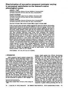
The preceding optimizations can be compared using the specific example of an eight-microphone linear array with ␭/4 sensor spacing. The array is focused at a distance equal to the array length, L, in the broadside direction 共␪⫽␲/2兲, as illustrated in Fig. 3. The noise correlation matrix is defined as in Eq. 共6兲 with Q being the correlation matrix corresponding to a spherically isotropic field26 and ␦ 2 ⫽0.0103. This value of ␦ 2 results in a white noise gain of 0 dB in the unconstrained optimized beamformer 关designed according to Eq. 共4兲兴. Since Rnn contains both a spherically isotropic portion as well as a spatially incoherent portion, the exact (cos ␥)2 for S and N will be somewhere in between the extremes depicted in Fig. 2. For an angle of incidence of ␲/2, (cos ␥)2⫽0.4 when Rnn ⫽Q and (cos ␥)2⫽0.8 when Rnn ⫽I. Three beamformers are considered: an unconstrained optimum, a null-constrained optimum, and a constrained opJ. G. Ryan and R. A. Goubran: Optimum near-field performance

2252

FIG. 3. Illustration of an eight-element, equispaced linear array and nearfield focal-point position.

timum with reduced interference suppression.

A. Unconstrained optimum

The unconstrained optimum beamformer is designed according to Eq. 共4兲 with no auxiliary constraints on the response pattern. Near-field and far-field beampatterns for the optimized array are shown in Fig. 4. The near-field beampattern is evaluated at a distance r equal to the focal distance L. It can be seen that the beamformer exhibits a pronounced peak in the response at the correct focal point. It is also seen that the far-field response pattern 共evaluated at r⫽⬁) is less directional but still responds strongly in the focal direction 共␲/2兲. The array gain for this case is 6.6 dB.

B. Null constrained

The next example is a beamformer optimized subject to a null constraint in the far-field direction as described by Eq. 共13兲. Beampatterns for the null-constrained optimum design are shown in Fig. 5. These should be compared with similar beampatterns obtained for the unconstrained optimum array shown in Fig. 4. The null-constrained design provides the desired response at the focal point; however, the near-field beampattern possesses somewhat higher sidelobe levels. In keeping with the null constraint, the far-field beampattern displays a sharp null in the response in the broadside direction. The cost of this added null in the far-field pattern is evident in the array gain which is reduced from 6.6 dB, for the unconstrained case, down to 2.3 dB a loss of 4.3 dB. This is within the range of 2.2 to 7.2 dB predicted by the ␣⫽⫺⬁ dB curve in Fig. 1. Furthermore, the null-constrained beam2253


FIG. 4. Near-field and far-field beampatterns for an eight-element uniformly spaced linear array with ␭/4 sensor spacing. The array is focused at (r f , ␪ f )⫽(L, ␲ /2) and the beampattern is evaluated at distances r⫽L 共a兲 and r⫽⬁ 共b兲.

former also possesses reduced robustness. The white noise gain is reduced by 10.4 dB compared to the unconstrained example.

C. Constrained to limit gain reduction

Beampatterns for the same array but designed using the constraint in Eq. 共14兲 are shown in Fig. 6. For this example, the constraint parameter ␣ is set to ⫺6 dB. Incorporating the soft constraint lessens the impact on the near-field beampattern’s sidelobe levels compared to the null constraint. Furthermore, the far-field response has been reduced by the ⫺6 dB compared to the beampattern in Fig. 4, as expected. The benefit of the soft constraint is that, in this case, the array gain is reduced by only 1.6 dB. This is in keeping with the predicted loss of between 0.7 and 3.1 dB. Furthermore, the white noise gain reduction is limited to 6.4 dB, resulting in a more-robust design. J. G. Ryan and R. A. Goubran: Optimum near-field performance

2253

FIG. 5. Beampatterns for the same array as in Fig. 4 but using linearly constrained optimal weights. Array gain is optimized while forcing a null in the broadside direction. The beampattern is evaluated at distances r⫽L 共a兲 and r⫽⬁ 共b兲.

V. CONCLUSIONS

This article addresses the problem of maximizing the near-field gain of a microphone array subject to a constraint on the far-field beampattern. It specifically addresses situations where the near-field signal source and the far-field interference are located along the same angle of incidence with respect to the array axis and both are immersed in a spherically isotropic field. This arises in speech pickup in rooms, for example, when a strong wall reflection or noise source originates from a location behind the near-field talker. When the angles of incidence from the near-field target and the far-field interference are identical, enforcing a null constraint in the interference direction reduces array gain and robustness. This article shows that this effect can be mitigated by proper selection of the beampattern constraint in the interference direction. By constraining the beampattern in the interference direction to be proportional to that of the unconstrained beampattern a minimum loss in array gain and robustness are achieved. The proportionality constant can 2254


FIG. 6. Soft-constrained optimum beampatterns for the array in Fig. 4. Array gain is optimized while suppressing the response in the broadside direction by an additional 6 dB compared to that shown in Fig. 4. The beampattern is evaluated at distances r⫽L 共a兲 and r⫽⬁ 共b兲.

then be used to trade off interference reduction and array gain. Using the example of an eight-element linear array focused in the broadside direction, the beampatterns and array gain of unconstrained and linearly constrained optimum beamformers are compared. Forcing a null in the interference direction results in a gain reduction of 4.3 dB. By constraining the interference to a level 6 dB below the unconstrained beamformer, the loss in array gain is limited to 1.6 dB. The new constraint also results in a more robust beamformer as indicated by the white noise gain. ACKNOWLEDGMENTS

The authors would like to thank Dr. M. R. Stinson of the National Research Council of Canada for helpful comments on an earlier version of this manuscript. 1

J. G. Ryan, ‘‘Criterion for the minimum source distance at which planewave beamforming can be applied,’’ J. Acoust. Soc. Am. 104, 595–598 共1998兲.


2254

2

M. M. Goulding and J. S. Bird, ‘‘Speech enhancement for mobile telephony,’’ IEEE Trans. Veh. Technol. 39, 316–326 共1990兲. 3 S. Nordholm, I. Claesson, and B. Bengtsson, ‘‘Adaptive Array Noise Suppression of Handsfree Speaker Input in Cars,’’ IEEE Trans. Veh. Technol. 42, 514–518 共1993兲. 4 F. Khalil, J. P. Jullien, and A. Gilloire, ‘‘Microphone Array for Sound Pickup in Teleconference Systems,’’ J. Audio Eng. Soc. 42, 691–700 共1994兲. 5 F. Pirz, ‘‘Design of a Wideband, Constant Beamwidth, Array Microphone for Use in the Near Field,’’ Bell Syst. Tech. J. 58, 1839–1850 共1979兲. 6 R. A. Kennedy, T. Abhayapala, and D. B. Ward, ‘‘Broadband nearfield beamforming using a radial beampattern transformation,’’ IEEE Trans. Signal Process. 46, 2147–2156 共1998兲. 7 D. B. Ward and G. W. Elko, ‘‘Mixed near-field/far-field beamforming: A new technique for speech acquisition in a reverberant environment,’’ Proc. IEEE Workshop on Applications of Signal Processing to Audio and Acoustics 1997, October 1997. 8 S. Nordholm, V. Rehbock, K. L. Teo, and S. Nordebo, ‘‘Chebyshev optimization for the design of broadband beamformers in the near field,’’ IEEE Trans. Circuits Syst. II: Analog Digital Signal Process. 45, 141–143 共1998兲. 9 J. G. Ryan and R. A. Goubran, ‘‘Array optimization applied in the near field of a microphone array,’’ IEEE Trans. Speech Audio Process 8, 173– 176 共2000兲. 10 C. Drane and J. McIlvenna, ‘‘Gain Maximization and Controlled Null Placement Simultaneously Achieved in Aerial Array Patterns,’’ Radio Electron. Eng. 39, 49–57 共1970兲. 11 A. Fenwick, ‘‘An array processor subject to a constraint,’’ J. Acoust. Soc. Am. 49, 1108–1110 共1971兲. 12 P. C. K. Kwok and P. S. Brandon, ‘‘Maximization of signal/noise ratio in antenna arrays subject to constraints,’’ Proc. Inst. Electr. Eng. 126, 1241– 1244 共1979兲. 13 T. S. Ng, J. Y. Chong Cheah, and F. J. Paoloni, ‘‘Optimization with

2255


controlled null placement in antenna array pattern synthesis,’’ IEEE Trans. Antennas Propag. 33, 215–217 共1985兲. 14 P. J. Kootsookos, D. B. Ward, and R. C. Williamson, ‘‘Imposing pattern nulls on broadband array responses,’’ J. Acoust. Soc. Am. 105, 3390– 3398 共1999兲. 15 J. T. Mayhan and L. J. Ricardi, ‘‘Physical limitations on interference reduction by antenna pattern shaping,’’ IEEE Trans. Antennas Propag. 23, 639–646 共1975兲. 16 H. Steyskal, ‘‘Synthesis of antenna patterns with prescribed nulls,’’ IEEE Trans. Antennas Propag. 30, 273–279 共1982兲. 17 T. S. Ng, ‘‘Equivalence of null constrained optimization problems in antenna array pattern synthesis,’’ J. Electr. Electron. Eng., Aust. 7, 302–305 共1987兲. 18 H. Steyskal, ‘‘Synthesis of antenna patterns with imposed near-field nulls,’’ Electron. Lett. 30, 2000–2001 共1994兲. 19 B. D. Van Veen and K. M. Buckley, ‘‘Beamforming: a versatile approach to spatial filtering,’’ IEEE Signal Process. Mag. , 4–24 共1988兲. 20 H. Cox, ‘‘Resolving power and sensitivity to mismatch of optimum array procesors,’’ J. Acoust. Soc. Am. 54, 771–785 共1973兲. 21 R. A. Monzingo and T. A. Miller, Introduction to Adaptive Arrays 共Wiley, New York, 1980兲. 22 D. K. Cheng and F. I. Tseng, ‘‘Gain optimization for arbitrary antenna arrays,’’ IEEE Trans. Antennas Propag. 13, 973–974 共1965兲. 23 J. M. Kates, ‘‘Superdirective arrays for hearing aids,’’ J. Acoust. Soc. Am. 94, 1930–1933 共1993兲. 24 R. W. Stadler and W. M. Rabinowitz, ‘‘On the Potential of fixed arrays for hearing aids,’’ J. Acoust. Soc. Am. 94, 1332–1342 共1993兲. 25 W. Soede, F. A. Bilsen, and A. J. Berkhout, ‘‘Development of a directional hearing instrument based on array technology,’’ J. Acoust. Soc. Am. 94, 785–798 共1993兲. 26 C. T. Morrow, ‘‘Point-to-point correlation of sound pressures in reverberation chambers,’’ J. Sound Vib. 16共1兲, 29–42 共1971兲.


2255

Using JASA format

Using JASA format

Suggest Documents