Using JASA format - Microsoft

Spontaneous speech recognition using a statistical coarticulatory model for the vocal-tract-resonance dynamics Li Denga) and Jeff Ma Department of Electrical and Computer Engineering, University of Waterloo, Waterloo, Ontario N2L 3G1, Canada

共Received 9 September 1999; revised 20 June 2000; accepted 7 August 2000兲

OF

O PR

A statistical coarticulatory model is presented for spontaneous speech recognition, where knowledge of the dynamic, target-directed behavior in the vocal tract resonance is incorporated into the model design, training, and in likelihood computation. The principal advantage of the new model over the conventional HMM is the use of a compact, internal structure that parsimoniously represents long-span context dependence in the observable domain of speech acoustics without using additional, context-dependent model parameters. The new model is formulated mathematically as a constrained, nonstationary, and nonlinear dynamic system, for which a version of the generalized EM algorithm is developed and implemented for automatically learning the compact set of model parameters. A series of experiments for speech recognition and model synthesis using spontaneous speech data from the Switchboard corpus are reported. The promise of the new model is demonstrated by showing its consistently superior performance over a state-of-the-art benchmark HMM system under controlled experimental conditions. Experiments on model synthesis and analysis shed insight into the mechanism underlying such superiority in terms of the target-directed behavior and of the long-span context-dependence property, both inherent in the designed structure of the new dynamic model of speech. © 2000 Acoustical Society of America. 关S0001-4966共00兲02911-8兴

I. INTRODUCTION

nology in accounting for the acoustic variability in spontaneous speech, which has been based on ever-expanding the myriad Gaussian mixture components and HMM states in a largely unstructured manner. 共This has a small number of exceptions; e.g., Ref. 3.兲 A particular model we have developed for this purpose describes the long-term 共utterancelength兲 context-dependent or coarticulatory effects in spontaneous speech in the domain of partially hidden vocal-tractresonance 共VTR兲. The VTR domain is internal to the domain of surface acoustic observation 共such as Mel-frequency cepstral coefficients or MFCCs兲. This coarticulation modeling is accomplished via two separate but related mechanisms. First, the mechanism of duration-dependent phonetic reduction allows the VTR variables and the associated surface acoustic variables to be modified automatically according to the varying speech rate and hence the duration of the speech units 共e.g., phones兲. This modification is physically established according to the structured dynamics assigned to the VTR variables in the model. Second, the ‘‘continuity’’ mechanism at the utterance level employed in the model constrain the VTR variables so that they flow smoothly from one segmental unit to another. Since this continuity constraint is global 共i.e., temporally across an entire utterance兲, long-span coarticulation is accomplished without the need to use explicit contextdependent units such as triphones. 共Use of triphone units is a main factor contributing to the success of current speech recognition technology for read-style speech, but at the expense of requiring unreasonable amounts of training data for the recognizers’ very large number of free parameters. This aspect of the weakness is completely eliminated by the coarticulatory model described in this article.兲 As a result, the

PY

CO

PACS numbers: 43.72.⫺p 关DOS兴

J. Acoust. Soc. Am. 108 (5), Pt. 1, Nov 2000

0001-4966/2000/108(5)/1/13/$17.00

S

1

JA 11

Current address: Li Deng, Microsoft Research, One Microsoft Way, Redmond, WA 98052. Electronic mail: [email protected]

90

a兲

02

Speech recognition technology has achieved significant success using complex models with their parameters automatically trained from large amounts of data.1 The success based on such an approach, however, has not been extended to spontaneous speech, which exhibits a much greater degree of variability than the less natural speech style for which the current technology has been successful. For the Switchboard spontaneous speech recognition task, even with use of hundreds of hours of speech as training data, the state-of-the-art, hidden Markov model 共HMM兲-based recognizers still produce more than one-third of errors in the recognized words.2 In order to capture the overwhelming variability in spontaneous, conversational speech, it appears necessary to explore some underlying structure in the speech patterns. The fundamental nature of the current acoustic modeling strategy used in the current technology is such that it explores only the surface-level observation data and not their internal structure or generative mechanisms. Because the variability in spontaneous speech is continuously scaled 共rather than discretely scaled兲, an infinite amount of surface-level data would be required, at least in theory, to completely cover such variability without using structural information. The research reported in this article represents our recent efforts in developing structural models for dynamic patterns of spontaneous speech. The goal of this research is to overcome the inadequacy of the current speech recognition tech-

© 2000 Acoustical Society of America

1

OF

O PR

number of free parameters for the recognizer and the amount of data required for training the recognizer are drastically reduced compared with the conventional HMM-based speech recognizers The organization of this article is as follows. In Sec. II, a detailed description of our new VTR-based statistical coarticulatory model will be provided. The learning algorithm we have developed for training the model parameters and a scoring algorithm will be presented in Sec. III. A series of experiments conducted for analysis, synthesis, and recognition of Switchboard spontaneous speech using the new coarticulatory model will be reported in Sec. IV. These will include detailed examinations of the model behavior in fitting the Switchboard data and of the quality of the spontaneous speech artificially generated from the model. They also include some small-scale N-best rescoring experiments used to diagnose the cause and nature of the recognition errors, as well as some large-scale N-best rescoring experiments, which provide the performance figures of the new recognizer. II. A STATISTICAL COARTICULATORY MODEL

CO

In this section, we provide a detailed account of the new speech model we have developed, including the motivation for the model development, the mathematical formulation of the model, and comparisons of the new model with other types of speech models used in the past. A. Background, motivation, and model overview

PY

any local temporal region are in combination exerting their influences on the VTR variable values 共and hence the acoustic observations as a noisy nonlinear functions of the VTR values兲 anywhere in the utterance. This gives rise to the property of long-term context dependence in the model without requiring use of context dependent speech units. Some background work, which leads to the development of this particular version of the model 共i.e., with use of VTRs as the partially hidden dynamic states兲, has been the extensive studies of spontaneous speech spectrograms and of the associated speech production mechanisms. The spectrographic studies on spontaneous speech have highlighted the critical roles of smooth, goal-directed formant transitions 共in vocalic segments, including vowels, glides, and liquids兲 in carrying underlying phonetic information in the adjacent consonantal and vocalic segments. The smoothness in formant movements 共for vocalic sounds兲 and in VTR movements 共for practically all speech sounds兲 reflects the dynamic behavior of the articulatory structure in speech production. The smoothness is not only confined within phonetic units but also across them. This cross-unit smoothness or continuity in the VTR domain becomes apparent after one learns to identify, by extrapolation, the ‘‘hidden’’ VTRs associated with most consonants, where the VTRs in spectrograms are either masked or distorted by spectral zeros, wide formant bandwidths, or by acoustic turbulences. The properties of the dynamic behavior change in a systematic manner as a function of speaking style and speaking rate, and the contextual variations of phonetic units are linked with the speaking style and rate variations in a highly predictable way. The VTRs are pole locations of the vocal tract configured to produce speech sounds. They have acoustic correlates of formants which are directly measurable for vocalic sounds, but often are hidden or perturbed for consonantal sounds due to the concurrent spectral zeros and turbulence noises. Hence, formants and VTRs are related but distinct concepts: the former is defined in the acoustic domain and the latter is associated with the vocal-tract properties per se. According to the goal-based speech production theory, articulatory structure and the associated VTRs necessarily manifest asymptotic behavior in their temporally smooth dynamics. This dynamic component of the overall speech model for the goal-directed and temporally smooth properties of the VTRs is called the 共continuous兲 ‘‘state’’ model. Since the temporal dynamics in the VTR variables is distorted, or hidden, in the observable acoustic signal, the overall speech-generative model needs to account for the physical, ‘‘quantal’’ nature of the distortion.4 This component of the model is called the ‘‘observation’’ model. In the current implementation of the model, the ‘‘observation’’ model for the distortion is constructed functionally by a static nonlinear function, implemented by artificial neural networks, mapping from the underlying VTRs to acoustic observations 共MFCCs in the current system兲. Since the same VTRs may produce drastically different MFCCs depending on whether the VTR共s兲 are hidden by spectral zero共s兲 or other factors, separate networks are used for distinct classes of speech sounds where each class corresponds to similar VTR-to-MFCC mappings. 共For example, the effects of nasal

S

JA 11

J. Acoust. Soc. Am., Vol. 108, No. 5, Pt. 1, Nov 2000

90

2

02

The statistical coarticulatory model presented in this article is a drastic departure from the conventional HMMbased approach to speech recognition. In the conventional approach, the variability in observed speech acoustics is accounted for by a large number of Gaussian distributions, each of which may be indexed by a discrete ‘‘context’’ factor. The discrete nature of encoding the contextual 共or coarticulatory兲 effect on speech variability leads to explosive growth of free parameters in the recognizers, and when the true source of the variability originates from causes of a continuous nature 共such as in spontaneous speech兲, this approach necessarily breaks down. In contrast, the new approach we have developed focuses directly on the continuous nature of speech coarticulation and speech variability in spontaneous speech. In particular, the phonetic reduction phenomenon is explicitly modeled by a statistical dynamic system in the domain of the VTR, which is internal to, or hidden from, the observable speech acoustics. In this dynamic model, the system matrix 共encompassing the concept of time constants兲 is structured and constrained to ensure the asymptotic behavior in the VTR dynamics within each speech segment. 关In the work reported in this article, we take speech segments as phones defined in the HMM systems on Switchboard tasks as used in the 1997 Workshop on Innovative Techniques for Large Vocabulary Conversational Speech Recognition 共http://www.clsp.jhu.edu/ws97/ws97គgeneral.html兲.兴 Across speech segments in a speech utterance, a smoothness or continuity constraint is imposed on the VTR variables. The main consequence of this constraint is that the interacting factors of phonetic context, speaking rate, and segment duration at

L. Deng and J. Ma: Spontaneous speech recognition

2

OF

O PR

coupling are represented by a neural network separate from all other non-nasal speech sounds.兲 Note that this static nonlinear function is clearly separated from the smooth-dynamic model describing the temporal asymptotic behavior for the underlying, hidden VTR dynamic variables. This separation makes it unnecessary, at least in principle, to extract formants from the speech signal in implementing the recognizer. But when formant information is made available with reliability indicator, this information can be and has been effectively used to initialize the model’s continuous ‘‘states’’ for the vocalic segments, and has been used in the overall statistical structure 共separate static nonlinear and dynamic linear components兲 of the model to facilitate model parameter learning. 共For example, to diagnose the accuracy of the state-estimation algorithm, we examine the algorithm’s output with reference to the formants extracted from vocalic segments in the training data; see Sec. III.兲 One key characteristic of this model is the elimination of the need to enumerate contextual factors such as triphones. The contextual variations are automatically built into the goal-directed, globally smooth dynamic ‘‘state’’ equations governing the VTR movements during speech utterances. Moreover, the contextual variations are integrated into speaking rate variations which are controlled by a small number of shared dynamic model parameters. The sharing is based on physical principles of speech production. To provide an overview, we have proposed a new coarticulatory speech model, which consists of two separate components. They accommodate separate sources of speech variability. The first component has a smooth dynamic property, and is linear but nonstationary. The nonstationarity is described by left-to-right regimes corresponding to sequentially organized phonological units such as context-independent phones. Handling nonstationarity in this way is very close to the conventional HMMs; but for each state 共discrete as in the HMM兲, rather than having an i.i.d. process, the new model has a phonetic-goal-directed linear dynamic process with the physically meaningful entity of continuous state variables. Equipped with the physical meaning of the state variables 共i.e., VTRs in the current version of the model兲, variability due to phonetic contexts and to speaking styles is naturally represented in the model structure with duration-dependent physical variables and with global temporal continuity of these variables. This contrasts with the conventional HMM approach where the variability is accounted for in a largely unstructured manner by accumulating an ever-increasing model size in terms of the number of Gaussian mixture components. 共The increase in the model size is blocked only by use of decision-tree based methods, at the expense of sacrificing modeling accuracy.兲 The second component, the observation model, is static and nonlinear. This lower-level component in the speech generation chain handles other types of variability including spectral tilts, formant bandwidths, relative formant magnitudes, frication spectra, and voice source differences. The two components combined form a nonstationary, nonlinear dynamic system whose structure and properties are well understood in terms of the general process of human speech production.

B. Mathematical formulation

The coarticulatory speech model with its overview provided in the preceding subsection has been formulated in statistical and mathematical terms as a constrained and simplified nonlinear dynamic system. This is a special version of the general statistical hidden dynamic model described in Refs. 5 and 6 using the EM implementation technique. 关The special structure of the model was also motivated by the speech production model of Ref. 7 based on articulatory gestural representations. While our model structure is much simplified from that of Ref. 7, the new statistical formulation of the model 共rather than a deterministic model in Ref. 7兲 gives its power for use in speech recognition that no previous deterministic model is capable of. Another novelty of our model is its use of vocal tract resonances, rather than vocal tract constrictions, as the dynamic, hidden state variable. This makes it much easier to implement the model and the related recognizer.兴 The dynamic system model consists of two separate but related components: 共1兲 state equation and 共2兲 observation equation, which are described below. 1. State equation

Z 共 k⫹1 兲 ⫽⌽ j Z 共 k 兲 ⫹ 共 I⫺⌽ j 兲 T j ⫹W d 共 k 兲 ,

j⫽1,2,...,J P ,

共1兲

PY

CO

A noisy, causal, and linear first-order ‘‘state’’ equation is used to describe the three-dimensional 共F1, F2, and F3兲 VTR dynamics according to

S

JA 11

90


02

3

where Z(k) is the three-dimensional ‘‘state’’ vector at discrete time step k, ⌽ j and T j are the system matrix and goal 共or target兲 vector associated with dynamic regime j which is related to the initiation of dynamic patterns in phone j, and J P is the total number of phones in a speech utterance. 共See a derivation of this discrete-time state equation from the continuous-time system in Ref. 5. This is a first-order system since its state has a time lag of one only in the system definition.兲 Both ⌽ j and T j are a function of time k via their dependence on dynamic regime j, but the time switching points are not synchronous with the phone boundaries. 共Throughout this article, we define the phone boundary as the time point when the phonetic feature of manner of articulation switches from one phone to its next adjacent phone. The dynamic regime often starts ahead of the phone boundary in order to initiate the dynamic patterns of the new phone. This is sometimes called ‘‘look-ahead’’ or anticipatory coarticulation.兲 The time scale for evolution of dynamic regime j is significantly larger than that for time frame k. In Eq. 共1兲, W d (k) is the discrete-time state noise, modeled by an i.i.d., zero-mean, Gaussian process with covariance matrix Q. 关Diagonal covariance matrix Q has been used in the current model, independent of phones 共i.e., Q is tied across all phones兲.兴 The special structure in the state equation, which is linear in the state vector Z(k) but nonlinear with respect to its parameters ⌽ j and T j , in Eq. 共1兲 gives rise to two significant properties of the VTRs modeled by the state vector Z(k). The first property is local smoothness; i.e., the state vector Z(k) is smooth within the dynamic regime associated with L. Deng and J. Ma: Spontaneous speech recognition

3

O PR

each phone. The second, attractor or saturation, property is related to the target-directed, temporally asymptotic behavior in Z(k). This target-directed behavior of the dynamics described by Eq. 共1兲 can be seen by setting k→⬁, which forces the system to enter the local, asymptotic region where Z(k ⫹1)⬇Z(k). With the assumption of mild levels of noise W d (k), Eq. 共1兲 then directly gives the target-directed behavior in Z(k): Z(k)→T j . An additional significant property of the state equation is the left-to-right structure in Eq. 共1兲 for j⫽1,2,...,J P and the related global-smoothness characteristics. That is, the local smoothness in state vector Z(k) is extended across each pair of adjacent dynamic regimes, making Z(k) continuous or smooth across an entire utterance. This continuity constraint is implemented in the current model by forcing the state vector Z(k) at the end of dynamic regime j to be identical to the initial state vector for dynamic regime j⫹1. That is, the Kalman filter which implements optimal state estimation 共see details in Sec. III兲 for dynamic regime j⫹1 is initialized by the Z(k) value computed at the end of dynamic regime j.

冉

兺j W i j •g j 兺l w jl •Z l

g共 x 兲⫽

CO

共2兲

g ⬘ 共 x 兲 ⫽g 共 x 兲 „1⫺g 共 x 兲 ….

The Jacobian matrix for Eq. 共3兲, which will be needed for the extended Kalman filter 共EKF; see Sec. III A 3兲, can be computed in an analytical form:

冉冊 ⳵h1 ⳵Z1

⳵h1 ⳵Z2

⳵h1 ⳵Z3

⳵h2 ⳵Z1

⳵h2 ⳵Z2

⳵h2 ⳵Z3

]

]

]

共6兲

⳵ h 12 ⳵ h 12 ⳵ h 12 ⳵Z1 ⳵Z2 ⳵Z3

where H il 共 Z 兲 ⫽

冋

兺j W i j g 兺l w jl g 共 Z l 兲

册冋冉兺 1⫺g

l

w jl g 共 Z l 兲

冊册

w jl .

The use of the Jacobian above is motivated by the need to linearize the observation equation so that the KF equations can be applied. C. Comparison with other models

90

The mathematical model described earlier in this section can be viewed as a significant extension of the linear dynamic system model as a thus-far most general formulation of stochastic segment models for speech described in Ref. 8 and 9. The extension is in the following six major aspects. First, while maintaining linearity in the state equation, the observation equation is extended to a nonlinear one with use of physically motivated nonlinear functions. Second, special structures are built into the state equation to ensure the target-directed property. Third, a physically motivated ‘‘global’’ continuity constraint is imposed on the state variable across phone-correlated dynamic regimes, to provide the long-span context-dependent modeling capability. This makes the current model not just a ‘‘segment’’ model as defined mathematically in Ref. 9, but a ‘‘supersegment’’ model where the correlation structure in the model extends over an entire speech utterance. Fourth, the continuous state variable is endowed with a physically meaningful entity in the realistic speech process 共i.e., VTRs兲, which allows special structures to be built into the state equation and which has been instrumental in the model development 共especially in model initialization, learning, and diagnosis兲. In contrast, in the linear dynamic system model described in Refs. 8 and

S

JA 11


共5兲

02

4

共4兲

with its derivative

PY

where the acoustic observation O(k) is MFCC measurements computed from a conventional speech preprocessor, and V(k) is the additive observation noise modeled by an i.i.d., zero-mean, Gaussian process with covariance matrix R, intended to capture residual errors in the nonlinear mapping from Z(k) to O(k). 共Again, diagonal covariance matrix R has been used in the current model independent of phones.兲 The multivariate nonlinear mapping, h (r) 关 Z(k) 兴 , is implemented by multiple switching MLPs 共multi-layer perceptions兲, with each MLP associated with a distinct manner 共r兲 of articulation of a phone. A total of ten MLPs 共i.e., r ⫽1,2,...,10兲 are used in the experiments reported in this article. The nonlinearity is necessary because the physical mapping from VTR frequencies 关 Z(k) 兴 to MFCCs 关 O(k) 兴 is highly nonlinear in nature. The noise used in the model Eq. 共2兲 captures the effects of VTR bandwidths 共i.e., formant bandwidths for vocalic sounds兲 and relative VTR amplitudes on the MFCC values. These effects are secondary to the VTR frequencies but they nevertheless contribute to the variability of MFCCs. Such secondary effects are quantified by the determinant of matrix R, which, in combination with the relative size of the state noise covariance matrix Q, plays important roles in determining relative amounts of state prediction and state update in the state estimation procedure. In implementing the nonlinear function h 关 Z(k) 兴共omitting index r for clarity henceforth兲 in Eq. 共2兲, we used a MLP network of three linear input units 关Z(k) of F1, F2, and F3兴, of 100 nonlinear hidden units, and of 12 linear output units 关 O(k) of MFCC1-12兴. Denoting the MLP weights from input to hidden units as w jl , and the MLP weights from hidden to output units as W i j , we have

共3兲

,

1 1⫹exp共 ⫺x 兲

The observation equation in the dynamic system model developed is nonlinear, noisy, and static, and is described by O 共 k 兲 ⫽h 共 r 兲关 Z 共 k 兲兴 ⫹V 共 k 兲 ,

冊

where i⫽1,2,...,12 is the index of output units 共i.e., component index of observation vector O k 兲, j⫽1,2,...,100 is the index of hidden units, and l⫽1,2,3 is the index of input units. In Eq. 共3兲, the hidden units’ activation function is the standard sigmoid function

d h 共 Z 兲 ⫽ 关 H il 共 Z 兲兴 ⫽ H z共 Z 兲 ⬅ dZ

OF

2. Observation equation

h i共 Z 兲 ⫽


4

OF

O PR

9, the continuous state variable was treated merely as a smoothed version of the noisy acoustic observation. Fifth, due to the introduction of nonlinearity in the observation equation and of the structural constraints in the state equation, the model learning and scoring algorithms described in Refs. 8 and 9 have been substantially extended. Finally, due to the compact structure in the current model for speech coarticulation and its elimination of explicit contextdependent units such as triphones, very small amounts of training data are needed for model parameter learning. In contrast, the model described in Refs. 8 and 9 still requires as much training data as the conventional HMM-based recognizers. Compared with other models of speech developed earlier in our laboratory, the current model offers several significant advantages. The articulatory-dynamic model and task-dynamic model described in Refs. 10–12 all have the dynamic state variables completely hidden 共i.e., unobservable兲. In the case of articulatory-dynamic model, the state variables are articulatory parameters, and in the case of the task-dynamic model, the state variables are vocal tract constriction parameters. The current model uses VTRs as the partially hidden state variables, which are observable for vocalic sounds. In addition to the smaller dimensionality in the dynamic system state 共three versus a dozen or so兲, use of the partially observable VTRs as the system state has been critically important in the model development 共model learning and diagnosis兲 and in the recognizer implementation. Further, use of the learnable MLP architecture for the observation equation provides significant implementation advantages over the earlier use of codebook methods. The acousticdynamic models described in Refs. 13–15, on the other hand, lack the physically meaningful internal dynamics, which is capable of piecing together phones in an utterance. Hence, despite the simplicity in the model development and recognizer implementation, it still requires explicit contextdependent units and therefore a large amount of training data. It shares similar weaknesses to those in the model described in Refs. 8 and 9. The current model shares similar motivations and philosophies of other work aiming at developing better, more compact coarticulatory models than the HMM. The models described in Refs. 16–19 have all used fully hidden internal dynamics, similar to the models described in Refs. 10–12. Some models explicitly use articulatory parameters as the dynamic variable 共e.g., Ref. 16兲, others use more abstract, automatically extracted variables for the purpose of modeling coarticulation 共e.g., Refs. 17–19兲. One main difference between these and the model described in this article lies in mathematical formulation of the models. The models described in Refs. 16, 17, and 19 are largely deterministic, where the outputs of the models need to be explicitly synthesized and compared with the unknown speech in order to reach recognition decision. In contrast, the statistical nature of the current model permits likelihood-score computation against the unknown speech 共similar to the conventional HMM formulation in this aspect兲 directly from the model parameters where the model synthesis is only carried out implicitly. In addition, the deterministic and statistical na-

tures render the models with different learning criteria and hence different learning algorithms.

III. LEARNING AND LIKELIHOOD-SCORING ALGORITHMS

In this section, we will describe the learning and likelihood-scoring algorithms we have developed for the statistical coarticulatory model for fixed dynamic regimes 共segmentations兲. These algorithms enable the training of the recognizer and the use of the recognizer for rescoring N-best hypotheses. A. Learning algorithm

PY

CO

The learning or parameter estimation method for the new speech model is based on the generalized EM algorithm. The EM algorithm is a two-step iterative scheme for maximum likelihood parameter estimation. Each iteration of the algorithm involves two separate steps, called the expectation step 共E-step兲 and the maximization step 共M-step兲, respectively. A formal introduction of the EM algorithm appeared in Ref. 20. Examples of using the EM algorithm in speech recognition can be found in Refs. 8, 13, and 19. The algorithm guarantees an increase 共or strictly speaking, nondecrease兲 of the likelihood upon each iteration of the algorithm and guarantees convergence of the iteration to a stationary point for an exponential family. Use of local optimization, rather than the global optimization, in the M step of the algorithm gives rise to the generalized EM algorithm. To derive the EM algorithm for the new model, we first use the i.i.d. noise assumption for W d (k) and V(k) in Eqs. 共1兲 and 共2兲 so as to express the log-likelihood for acoustic observation sequence O⫽ 关 O(1),O(2),...,O(N) 兴 and hidden task-variable sequence Z⫽ 关 Z(1),Z(2),...,Z(N) 兴 as

90

1 ⫽⫺ 2

N⫺1

兺

兵 log 兩 Q 兩 ⫹ 关 Z 共 k⫹1 兲 ⫺⌽Z 共 k 兲 ⫺ 共 I⫺⌽ 兲 T 兴 ⬘

JA 11

k⫽0

⫻Q ⫺1 关 Z 共 k⫹1 兲 ⫺⌽Z 共 k 兲 ⫺ 共 I⫺⌽ 兲 T 兴其 N

1 ⫺ 兵 log 兩 R 兩 ⫹ 关 O 共 k 兲 ⫺h„Z 共 k 兲 …兴 ⬘ R ⫺1 2 k⫽1

兺

⫻ 关 O 共 k 兲 ⫺h 共 Z 共 k 兲兲兴其 ⫹const,

S


02

5

log L 共 Z,O,⌰ 兲

where superscript ⬘ denotes matrix transposition, and the model parameters ⌰ to be learned include those in the state equation 共1兲 and those in the MLP nonlinear mapping functions Eq. 共2兲: ⌰⫽ 兵 T,⌽,W i j ,w jl ,i⫽1,2,...,I; j⫽1,2,...,J;l ⫽1,2,...,L 其 . 共To simplify the algorithm description without loss of generality, estimation of additional model parameters of covariance matrices Q, R for state and observation noises will not be addressed in this article. Also, the dynamicregime index on parameters T, ⌽ and the phone-class index on parameters W i j , w jl are dropped because supervised learning is used. In the current model implementation, I ⫽3, J⫽100, L⫽12.兲 L. Deng and J. Ma: Spontaneous speech recognition

5

1. E-step

N

兺

The E-step of the EM algorithm involves computation of the following conditional expectation 共together with a set of related sufficient statistics needed to complete evaluation of the conditional expectation兲: Q 共 Z,O,⌰ 兲 ⫽E 兵 log L 共 Z,O,⌰ 兲兩 O,⌰ 其 ⫽⫺

N⫺1

兺

k⫽0

N

兺

冏册

N⌽TT ⬘ ⫺⌽TA ⬘ ⫺⌽AT ⬘ ⫺NTT ⬘ ⫺TA ⬘

⬘ Q ⫺1 e k1 兩 O,⌰ 兴 E 关 e k1

⫹BT ⬘ ⫹⌽C⫺D⫽0,

1 ⬘ R ⫺1 e k2 兩 O,⌰ 兴 , E 关 e k2 2 k⫽1

兺

共12兲

where

O PR

N⫺1

where e k1 ⫽Z(k⫹1)⫺⌽Z(k)⫺(I⫺⌽)T and e k2 ⫽O(k) ⫺h(Z(k)), and E denotes conditional expectation on observation vectors O. This can be simplified, by substituting the optimal values of covariance matrix estimates, to

A⫽

N⫺1

兺

E 关 Z 共 k 兲兩 O,⌰ 兴 ,

k⫽0

B⫽

兺

k⫽0

E 关 Z 共 k⫹1 兲兩 O,⌰ 兴 ,

N⫺1

C⫽

OF

兺

E 关 Z 共 k 兲 Z 共 k 兲 ⬘ 兩 O,⌰ 兴 ,

k⫽0 N⫺1

D⫽

兺

k⫽0

N⌽ ⬘ ⌽T⫺⌽ ⬘ ⌽A⫺N⌽ ⬘ T⫺N⌽T⫹⌽ ⬘ B 共13兲

The coefficients in Eqs. 共12兲 and 共13兲, A, B, C, and D, constitute the sufficient statistics, which can be obtained by the standard technique of EKF 共see Sec. III A 3兲. Solutions to Eqs. 共10兲 and 共11兲 for finding (W i j ,w jl ) to maximize Q 2 in Eq. 共7兲 have to rely on approximation due to the complexity in the nonlinear function h(Z). The approximation involves first finding estimates of hidden variables Z(k), Z(k 兩 k), via the EKF algorithm. Given such estimates, the conditional expectations in Eqs. 共10兲 and 共11兲 are approximated to give

JA 11

90

2. M-step

⫹⌽A⫹NT⫺B⫽0.

02

共For detailed derivation, see Ref. 21.兲 Note that the stateequation’s parameters (⌽,T) are contained in Q 1 only and the MLP weight parameters (W i j ,w jl ) in the observation equation are contained in Q 2 only. These two sets of parameters can then be optimized independently in the subsequent M-step to be detailed in Sec. III A 2.

E 关 Z 共 k⫹1 兲 Z 共 k 兲 ⬘ 兩 O,⌰ 兴 .

Equation 共9兲 is another third-order nonlinear algebraic equation 共in ⌽ and T兲 of the form

PY

CO 共7兲

N

N⫺1

冋

⳵Q1 ⳵ ⬀ E 兵关 Z 共 k⫹1 兲 ⫺⌽Z 共 k 兲 ⳵ ⌽ k⫽0 ⳵⌽

兺

冏册

⫺ 共 I⫺⌽ 兲 T 兴 2 其 O,⌰ ⫽0, N⫺1

冋

共8兲

⳵Q1 ⳵ E ⬀ 兵关 Z 共 k⫹1 兲 ⫺⌽Z 共 k 兲 ⳵ T k⫽0 ⳵T

兺

冏册

⫺ 共 I⫺⌽ 兲 T 兴 2 其 O,⌰ ⫽0, J. Acoust. Soc. Am., Vol. 108, No. 5, Pt. 1, Nov 2000

共9兲

⳵Q2 ⳵ h„Z 共 k 兩 k 兲 … ⬀ , 关 O 共 k 兲 ⫺h 共 Z 共 k 兩 k 兲兲兴 ⬘ ⳵ W i j k⫽1 ⳵Wij

兺 N

⳵Q2 ⳵ h„Z 共 k 兩 k 兲 … ⬀ . 关 O 共 k 兲 ⫺h 共 Z 共 k 兩 k 兲兲兴 ⬘ ⳵ w jl k⫽1 ⳵ w jl

兺

S

The M-step of the EM algorithm aims at optimizing the Q function in Eq. 共7兲 with respect to model parameters ⌰ ⫽ 兵 T,⌽,W i j ,w jl 其 . For the model at hand, it seeks solutions for

6

冋

共10兲

⳵Q2 ⳵ ⬀ E 兵关 O 共 k 兲 ⫺h 共 Z 共 k 兲兲兴 2 其 O,⌰ ⫽0. 共11兲 ⳵ w jl k⫽1 ⳵ w jl

N

⫺

冏册

Equation 共8兲 is a third-order nonlinear algebraic equation 共in ⌽ and T兲, of the following form after some algebraic and matrix-calculus manipulation:

N N log 兩 Q 兩 ⫺ log 兩 R 兩 2 2

1 ⫺ 2

冋

⳵Q2 ⳵ ⬀ E 兵关 O 共 k 兲 ⫺h 共 Z 共 k 兲兲兴 2 其 O,⌰ ⫽0, ⳵ W i j k⫽1 ⳵ W i j

共14兲

共15兲

If the estimated state variable, Z(k 兩 k), is treated as the input to the MLP neural network defined in Eq. 共3兲, and the observation, O(k), as the output of the MLP, then the gradients expressed in Eqs. 共14兲 and 共15兲 are exactly the same as those in the backpropagation algorithm.22 Therefore, the backpropagation algorithm is used to provide the estimates to W i j and w jl parameters. The local-optimum property of the backpropagation algorithm in this M-step makes the learning algorithm described in this section a generalized EM. The approximation used to obtain the gradients in Eqs. 共14兲 and 共15兲 makes the learning algorithm a pseudo-EM. L. Deng and J. Ma: Spontaneous speech recognition

6

3. Extended Kalman filter for finding sufficient statistics

OF

O PR

We have observed that in the E-step derivation of the EM algorithm shown in this section, the objective functions Q 1 and Q 2 in Eq. 共7兲 contain a set of conditional expectations as sufficient statistics. These conditional expectations, A, B, C, and D in Eqs. 共12兲 and 共13兲, need to be computed during the M-step of the EM algorithm. The extended Kalman filter or EKF algorithm provides a solution to finding these sufficient statistics. 共We have also implemented an extended Kalman smoothing algorithm which is expected to provide more accurate solutions. But in this work we have empirically observed no practical differences from the EKF. In this article we only describe the EKF method used.兲 Also, as shown in Sec. III A 2, the EKF algorithm is also needed to approximate the gradients in Eqs. 共10兲 and 共11兲, before the M-step can be formulated as the backpropagation algorithm and can be carried out straightforwardly. The EKF algorithm gives an approximate minimummean-square estimate to the state of a general nonlinear dynamic system. Our speech model discussed in Sec. II B uses a special structure within the general class of the nonlinear dynamic system models. Given such a structure, the EKF algorithm developed is described here in a standard predictor-corrector format.23,24 Denoting by Zˆ (k 兩 k) the EKF state estimate and by ˆZ (k⫹1 兩 k) the one-step EKF state prediction, the prediction equation for the special structure of our model has the form

CO

E 关 Z 共 k⫹1 兲兩 O 兴 ⫽Zˆ 共 k⫹1 兩 N 兲 ⬇Zˆ 共 k⫹1 兩 k⫹1 兲 , E 关 Z 共 k 兲 Z 共 k 兲 ⬘ 兩 O 兴 ⫽ P 共 k 兩 N 兲 ⫹Zˆ 共 k 兩 N 兲 Zˆ 共 k 兩 N 兲 ⬘ ⬇ P 共 k 兩 k 兲 ⫹Zˆ 共 k 兩 k 兲 Zˆ 共 k 兩 k 兲 ⬘ ,

共16兲

where K(k⫹1) is the filter gain computed recursively according to K 共 k⫹1 兲 ⫽ P 共 k⫹1 兩 k 兲 H z 关 Zˆ 共 k⫹1 兩 k 兲兴 ⫻ 兵 H z 关 Zˆ 共 k⫹1 兩 k 兲兴 P 共 k⫹1 兩 k 兲 H z

P 共 k⫹1 兩 k⫹1 兲 ⫽ 兵 I⫺K 共 k⫹1 兲 H z ⫻ 关 Zˆ 共 k⫹1 兩 k 兲兴其 P 共 k⫹1 兩 k 兲 . J. Acoust. Soc. Am., Vol. 108, No. 5, Pt. 1, Nov 2000

P 共 k⫹1,k 兩 k⫹1 兲

⫽ 关 I⫺K 共 k⫹1 兲 H z „Zˆ 共 k⫹1 兩 k⫹1 兲 …兴 ⌽ P 共 k 兩 k 兲 . It is noted that while the EM algorithm requires Kalman smoothing which takes into account the complete acoustic observation sequences, we found no practical differences with the use of Kalman filtering taking account of only the previous observations. In other words, we used the EKF to approximate the corresponding smoothing algorithm in computing all the sufficient statistics required by the EM algorithm. B. Likelihood-scoring algorithm for recognizer testing

⫻ 关 Zˆ 共 k⫹1 兩 k 兲兴 ⬘ ⫹R 共 k⫹1 兲其 ⫺1 , P 共 k⫹1 兩 k 兲 ⫽⌽ P 共 k 兩 k 兲 ⌽ ⬘ ⫹Q 共 k 兲 ,

All the quantities on the right-hand sides of the above are computed directly from the EKF recursion Eqs. 共16兲–共18兲, except for the quantity P(k⫹1,k 兩 k⫹1), which is computed separately according to

S

共17兲

⫹Zˆ 共 k⫹1 兩 k⫹1 兲 Zˆ 共 k 兩 k 兲 ⬘ .

JA 11

⫻ 兵 O 共 k⫹1 兲 ⫺h„Zˆ 共 k⫹1 兩 k 兲 …其 ,

⬇ P 共 k⫹1,k 兩 k⫹1 兲

90

Zˆ 共 k⫹1 兩 k⫹1 兲 ⫽Zˆ 共 k⫹1 兩 k 兲 ⫹K 共 k⫹1 兲

E 关 Z 共 k⫹1 兲 Z 共 k 兲 ⬘ 兩 O 兴 ⫽ P 共 k⫹1,k 兩 N 兲 ⫹Zˆ 共 k⫹1 兩 N 兲 Zˆ 共 k 兩 N 兲 ⬘

02

The physical interpretation of Eq. 共16兲 applied to our speech model is that the one-step EKF state predictor based on the current EKF state estimate will always move towards the target vector T for a given system matrix ⌽. Such desirable dynamics comes directly from state equation 共1兲, and it is, in fact, in exactly the same form as the noise-free model state equation. Denote by H z „Zˆ (k⫹1 兩 k)… the Jacobian matrix, as defined in Eq. 共6兲, at the point of Zˆ (k⫹1 兩 k) for the MLP observation equation in our speech model, and denote by h„Zˆ (k⫹1 兩 k)… the MLP output for the input Zˆ (k⫹1 兩 k). Then the EKF corrector 共or filter兲 equation applied to our speech model is

7

E 关 Z 共 k 兲兩 O 兴 ⫽Zˆ 共 k 兩 N 兲 ⬇Zˆ 共 k 兩 k 兲 ,

PY

Zˆ 共 k⫹1 兩 k 兲 ⫽⌽Zˆ 共 k 兩 k 兲 ⫹ 共 I⫺⌽ 兲 T.

In the above, P(k⫹1 兩 k) is the prediction error covariance and P(k⫹1 兩 k⫹1) is the filtering error covariance. The physical interpretation of Eq. 共17兲 as applied to our speech model is that the amount of correction to the state predictor obtained from Eq. 共17兲 is directly proportional to the accuracy with which the MLP is used to model the relationship between the state Z(k) or VTRs and the observation O(k) or MFCCs. 关Correction is necessary because the predictor obtained from Eq. 共16兲 is based solely on the system dynamics discarding the actual observation. Use of the actual observation will improve the accuracy of the state estimation.兴 Such a matching error in the acoustic domain 共called innovation in estimation theory24兲 is magnified by the timevarying filter gain K(k⫹1), which is dependent on the balance of the covariances of the two noises Q and R, and on the local Jacobian matrix which measures the sensitivity of the nonlinear function h(Z) represented by the MLP. In using the EM algorithm to learn the model parameters, we require that all the conditional expectations 共sufficient statistics兲 for the coefficients A, B, C and D in Eq. 共13兲 be reasonably accurately evaluated. This can be accomplished, once the EKF’s outputs become available, according to

共18兲

In addition to the use of the EKF algorithm in the model learning as discussed so far, it is also needed in the likelihood-scoring algorithm 共during the recognizer testing phase兲 which we discuss now. Using the basic estimation theory for dynamic systems 共cf. Theorem 25-1 in Ref. 24; see also in Ref. 8兲, the logL. Deng and J. Ma: Spontaneous speech recognition

7

likelihood scoring function for our speech model can be computed from the approximate innovation sequence ¯ (k 兩 k⫺1) according to O N

1 ¯ 共 k 兩 k⫺1 兲 ⬘ log L 共 O 兩 ⌰ 兲 ⫽⫺ 兵 log 兩 P O¯ O¯ 共 k 兩 k⫺1 兲兩 ⫹O 2 k⫽1

兺

⫺1 ¯ 共 k 兩 k⫺1 兲其 ⫹const, ⫻ P O¯ O¯ 共 k 兩 k⫺1 兲 O

共19兲

where the approximate innovation sequence ¯ 共 k 兩 k⫺1 兲 ⫽O 共 k 兲 ⫺h„Zˆ 共 k 兩 k⫺1 兲 …, O

k⫽1,2,...,N

is computed from the EKF recursion, and P O¯ O¯ is the covariance matrix of the approximate innovation sequence:

O PR

P O¯ O¯ 共 k 兩 k⫺1 兲 ⫽H z „Zˆ 共 k 兩 k⫺1 兲 …P 共 k 兩 k⫺1 兲 ⫻H z „Zˆ 共 k 兩 k⫺1 兲 …⬘ ⫹R,

OF

which is also computed from the EKF recursion. For a speech utterance which consists of a sequence of phones with the dynamic regimes given, the log-likelihood scoring functions for each phone in the sequence as defined in Eq. 共19兲 are summed to give the total log-likelihood score for the entire speech utterance.

CO

IV. SPEECH RECOGNITION, SYNTHESIS, AND ANALYSIS EXPERIMENTS

PY

In this section, we will report a series of experiments conducted for analysis, synthesis, and recognition of Switchboard spontaneous speech using the statistical, VTR-based coarticulatory model presented so far. After introducing the experimental paradigm and the design parameters of the new recognizer, we will first report a set of small-scale N-best rescoring speech recognition experiments, which permits analysis of the model behavior by manipulating some handtuned variables. We will then evaluate the performance of the new recognizer in a set of large-scale N-best rescoring experiment, and compare the performance figures with the conventional triphone HMM-based speech recognizer under similar conditions. Finally, we will present some modelsynthesis results and give detailed examinations of the model behavior in fitting the Switchboard data and of the quality of the spontaneous speech artificially generated from the model. Such analysis and synthesis experiments serve to explain why the new coarticulatory model is doing the right job in ‘‘locking into’’ the correct transcription but at the same time it can ‘‘break away’’ from partially correction transcriptions due to contextual influences.

model. The reasons for using the limited N-best rescoring paradigm in the current experiments are mainly due to computational ones. The benchmark HMM system used in our experiments is one of the best systems developed earlier 关see http:// www.clsp.jhu.edu/ws97/ws97គgeneral.html兲兴, and it has been described in some detail in Refs. 19 and 25. Briefly, the system has word-internal triphones clustered by a decision tree, with a bigram language model. The total number of the parameters in this benchmark HMM system is approximately 3 276 000, which can be broken down to the product of 共1兲 39, which is the MFCC feature vector dimension; 共2兲 12, which is the number of Gaussian mixtures for each HMM state; 共3兲 2, which includes Gaussian means and diagonal covariance matrices in each mixture component; and 共4兲 3500, which is the total number of the distinct HMM states clustered by the decision tree. In contrast, the total number of parameters in the new recognizer is considerably smaller. The total 15 252 parameters in the recognizer consists of those from target parameters 42⫻3⫽126, those from diagonal dynamic system matrices 42⫻3⫽126, and those from MLP parameters 10⫻100 ⫻共12⫹3兲⫽15 000. These numbers are elaborated later while detailing several essential implementation aspects of the recognizer. First, we choose a total of 42 distinct phonelike symbols, including 8 context-dependent phones, each of which is intended to be associated with a distinct three-dimensional 共F1, F2, and F3兲 vector-valued target (T j ) in the VTR domain. The phonelike symbol inventory and the VTR target values used to initialize the model training discussed in Sec. III A are based on the Klatt synthesizer setup.26 The values are slightly adjusted by examining some spectrograms of the Switchboard training data. Among the 42 phonelike symbols, 34 are context independent. The remaining eight are context dependent because their target VTRs are affected by the anticipatory tongue position associated with the following phone. The next set of model parameters is the elements in the 42 distinct diagonal dynamic system matrices (⌽ j ). Before the training, they are initialized based on the consideration that the articulators responsible for producing different phones have different intrinsic movement rates. This difference roughly translates to the difference in the VTR movement rates across the varying phones. For example, the VTR transitions for labial consonants 共/b/, /m/, /p/兲 marked by ‘‘Lips’’ features are significant faster than those for alveolar consonants 共/d/, /t/, /n/兲 marked by ‘‘Tongue-Blade’’ features. The VTR transitions for both labial and alveolar consonants are faster than those for velar consonants 共marked by ‘‘Tongue Dorsum’’ features兲 and those of vowels marked also by the ‘‘Tongue Dorsum’’ features. 共We found that after the model training, the differences in the elements of the system matrices are largely retained from the initialization across the phone classes. However, their values have been changed after the training.兲 The final set of model parameters in the recognizer are the MLP weights, W i j and w jl , responsible for the VTR-toMFCC mapping. Unlike the target and system matrix param-

S


JA 11

8

90

In all the experiments reported in this article, we used an N-best list rescoring paradigm, according to the scoring algorithm Eq. 共19兲, to evaluate the new recognizer based on the VTR-based coarticulatory model on the Switchboard spontaneous speech data. The N-best list of word transcription hypotheses and their phone-level segmentation 共i.e., alignment兲 are obtained from a conventional triphone-based HMM which also serves as the benchmark to gauge the recognizer performance improvement via use of the new speech

02

A. Experimental paradigm, HMM benchmark system, and design parameters of the VTR recognizer


8

OF

O PR

eters which are phone dependent, we tie the MLPs approximately according to the distinct classes of manner of articulation 共and voicing兲. Such tying reduces the MLP noise resulting from otherwise too many independently trained MLPs. On the other hand, by not tying all phones into one single MLP, we also ensure effective discrimination of phones using differential nonlinear mapping 共from the smoothed physical VTR state variables to the MFCCs兲 even if the VTR targets are identical for different phones 共a few phones have nearly identical VTR targets兲. The ten classes resulting from the tying and used in the current recognizer implementation are 共1兲 aw, ay, ey, ow, oy, aa, ae, ah, ao, ax, ih, iy, uh, uw, er, eh, el; 共2兲 l, w, r, y; 共3兲 f, th, sh; 共4兲 s, ch; 共5兲 v, dh, zh; 共6兲 z, jh; 共7兲 p, t, k; 共8兲 b, d, g; 共9兲 m, n, ng, en; and 共10兲 sil, sp. In the above tying scheme, all vowels are tied using one MLP, because vowel distinction is based exclusively on different target values in the VTR domain. Here /s/ and /sh/ are associated with separate MLPs, because their target VTR values 共not observable in the acoustic domain because of concurrent zeros and large VTR bandwidths兲 are similar to each other 关This can be seen in terms of their similar ways in attracting the VTR 共formant兲 transitions from the adjacent phones.兴 Hence their distinction will be based mainly on the different VTR-to-MFCC mappings. In this case, the acoustic difference between these two phones in terms of the greater amount of energy at lower frequency for /sh/ than for /s/ is captured by different MLP weights 共which are trained automatically兲, rather than by differential VTR target values since the behavior of attracting adjacent phones’ VTR transitions is similar between /s/ and /sh/. Now for each of the 10 distinct MLPs, we use 100 共nonlinear兲 hidden units, 3 共linear兲 input units, and 12 共linear兲 output units. This gives a total of 10⫻100⫻共3⫹12兲 MLP weight parameters.

TABLE I. Performance comparison of three recognizers for 18 utterances with the same speaker in training and testing 共ref⫹5兲.

% Reference-at-top Average word error rate

Benchmark HMM

VTR 共HMM align兲

VTR 共true align兲

37.0% 39.2%

38.8% 30.4%

50.0% 22.8%

PY

CO

eses; and 共3兲 VTR model using manually determined ‘‘true’’ dynamic regimes for the reference hypothesis according to spectrogram reading. A performance comparison of these three recognizers is shown in Table I. Two performance measures are used in this comparison. First, among the 18 test utterances we examine the percentage when the correct, reference hypothesis scores higher than all the remaining five hypotheses. Second, we directly compute the word error rate 共WER兲 using the standard NIST scoring software. The new, VTR-based recognizers are consistently better than the benchmark HMM, especially when the ‘‘true’’ dynamic regimes are provided and in this case the performance is considerably better. We conduct a similar experiment to the above, using the same recognizers trained from a single male but choosing a separate male speaker’s ten utterances as the test data. Again, as shown in Table II, the VTR-based recognizer with the ‘‘true’’ dynamic regimes gives significantly better performance than the others. These experiments demonstrate superior performance of the VTR-based coarticulatory model, when exposed to the reference transcriptions. They also highlight the importance of providing the true or optimal dynamic regimes to the model. Automatic searching for the optimal dynamic regimes is a gigantic computational problem and has not been addressed by the work reported in this article.

S


In the large-scale experiments, we keep the same recognizers trained from a single male speaker but significantly increase the size of the test set. All the male speakers from the WS’97 DevTest are selected, resulting in a total of 23 male speakers comprising 24 conversation sides 共each side has a distinct speaker兲, 1241 utterances 共sentences兲, 9970 words, and 50 min of speech as the test data. Because of the large test set and because of lack of an efficient method to automate the optimization of the VTR-model dynamic regimes, we report in this section only the performance comparison between the benchmark HMM recognizer and the VTR recognizer with dynamic regimes suboptimally derived from the HMM phone alignments. In Table III, we provide the performance comparison for the ‘‘ref⫹5’’ mode, and for

JA 11

9

C. Experiments on large-scale N-best rescoring

90

In this set of experiments, we train the VTR-based model with the design parameters outlined above using speech data from a single male speaker in the Switchboard data. A total of 30 min of the data are used which consist of several telephone conversations. Due to the use of only a single speaker, we avoid normalization problems for both the VTR targets and for the MFCC observations. We randomly selected 18 utterances 共sentences兲 in one conversation as the test data from the same speaker that are disjoint from the training set. For these 18 utterances, an N-best list with N⫽5 is generated, together with the phone alignments for each of the five-best hypotheses, by the benchmark HMM system. We then add the reference 共correct兲 hypothesis together with its phone alignments into this list, making a total of six 共‘‘ref⫹5’’兲 hypotheses to be rescored by the VTR recognizer. Under the identical conditions set out above, we rescore these 18 utterances using the following three recognizers with the language model removed: 共1兲 benchmark triphone HMM; 共2兲 VTR model using automatically computed phone alignments 共which determine the VTR dynamic regimes for each constituent phone兲 by the HMM for all the six hypoth-

02

B. Experiments on small-scale N-best rescoring

TABLE II. Performance comparison of three recognizers for ten utterances with separate speakers in training and testing 共ref⫹5兲.

% Reference-at-top Average word error rate

Benchmark HMM

VTR 共HMM align兲

VTR 共true align兲

30.0% 27.0%

40.0% 25.7%

50.0% 9.2%


9

TABLE III. Performance comparison of two recognizers for a total of 1241 test utterances when the recognizers are exposed to the reference transcription 共ref⫹5 and ref⫹100兲.

TABLE V. Performance comparison of two recognizers for a total of 1241 utterances when the recognizers are not exposed to the reference transcription 共5-best and 100-best兲.

Benchmark HMM

VTR 共HMM align兲

Chance

Benchmark HMM

VTR 共HMM align兲

Chance

44.8% 56.1%

32.3% 50.2%

45.0% 59.6%

52.6% 58.9%

51.8% 58.2%

54.0% 60.2%

Average WER 共ref⫹5兲 Average WER 共ref⫹100兲

OF

O PR

the additional ‘‘ref⫹100’’ mode where the N-best list contains 100 hypotheses. In Table III, we also add the ‘‘Chance’’ performance which is used to calibrate the recognizers’ performance. The chance WER is computed by ensemble averaging the WERs obtained by having a recognizer randomly choosing one hypothesis from the six possible ones 共for the ref⫹5 mode or N⫽5兲 or from the 101 possible ones 共for the ref⫹100 mode or N⫽100兲. For both the N ⫽5 and N⫽100 cases, the VTR recognizer performs significantly better than the benchmark HMM recognizer, which is slightly better than the chance performance. More detailed results of the above experiment for the VTR recognizer are shown in Table IV, where the average WER is shown as a function of N in the N-best list. We also conduct the same experiment as shown in Table III except no reference transcription is added into the N-best list. The results are shown in Table V, with N⫽5 and N ⫽100 in the N-best list, respectively. In the both cases, the VTR recognizer performs nearly the same as the chance, both slightly worse than the benchmark HMM recognizer. This contrasts sharply with the superior performance of the VTR recognizer when it is exposed to the reference transcription shown in Tables I–III. A reasonable explanation is that the long-span context-dependence property of the VTR model naturally endows the model with the capability to ‘‘lock-in’’ to the correct transcription and it at the same time increases the tendency for the model to ‘‘break-away’’ from partially correct transcriptions due to the influence of wrong contexts. Since nearly all the hypotheses in the N-best list contain a large proportion of incorrect words, they affect the matching of the model to the remaining correct words in the hypotheses through the context-dependence mechanism much stronger than the conventional triphone HMM. 共Professor Fred Jelinek pointed out to us that similar effects have been found in language modeling using long-span dependency language models.27兲

Average WER 共5-best兲 Average WER 共100-best兲

analysis of experimental results with physical insight and understanding. 共The conventional HMM would have a hard time of doing this because of its lack of physical structure in the model.兲 To pursue this analysis, we introduce the methodology of ‘‘model synthesis.’’ Model synthesis refers to the process of generating an ˆ (1),O ˆ (2),...,O ˆ (N), artificially observation sequence, O from the model conditioned on a fixed sequence of observation data, O(1),O(2),...,O(N), and on its transcription. When the model used is the current VTR model, we pursue the model-synthesis procedure as follows. First, given the fixed sequence of observation MFCC data, O(1), O(2),...,O(N), we apply the EKF algorithm to obtain the predicted VTR state sequence: Zˆ 共 1 兩 0 兲 ,Zˆ 共 2 兩 1 兲 ,...,Zˆ 共 k 兩 k⫺1 兲 ,...,Zˆ 共 N 兩 N⫺1 兲 .

PY

CO

The parameters in the VTR model used in the EKF algorithm are consistent with the phonelike transcription for the given MFCC data. The dynamic regime for each phonelike unit is fixed in advance, and in moving from one dynamic regime to the next, the continuity constraint is imposed on the VTR state while applying the EKF algorithm. Second, using the predicted VTR state sequence, we generate the MFCC sequence according to the nonlinear mapping:

02

ˆ 共 k 兲 ⫽h„Zˆ 共 k 兩 k⫺1 兲 …, O

k⫽1,2,...,N.

共20兲

S

JA 11

90

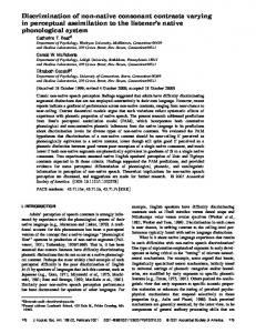
While using the MLPs to synthesize the MFCC sequence according to Eq. 共20兲, one of the ten MLPs is selected at each time frame depending on the given alignment of the phonelike units. The result of the VTR model synthesis applied to a Switchboard test utterance ‘‘And that’s mostly flat,’’ which is transcribed as sil, /ae/, /n/, /d/, /dh/, /ae/, /t/, /s/, /m/, /ow/, /s/, /t/, /l/, /f/, /l/, /ae/, /t/, sil, is shown in Fig. 1. It shows the speech waveform with phone segmentation 共top兲, the data MFCC sequence converted and then displayed in a Melscaled spectrogram format 共middle兲, and the VTR modelsynthesized MFCC sequence displayed also in the Melscaled spectrogram format 共bottom兲. The three-dimensional predicted VTR vector by the EKF algorithm, Zˆ (1 兩 0), Zˆ (2 兩 1),...,Zˆ (k 兩 k⫺1),...,Zˆ (N 兩 N⫺1), is superimposed on the model-synthesized Mel-scaled spectrogram. The VTRs give a reasonably good match to the spectral peaks derived from the MFCC sequence during all vocalic segments in the

D. Experiments on model synthesis and analysis

The experiments described in this section are devoted to investigating and demonstrating some intrinsic mechanisms responsible for the VTR-based, coarticulatory model’s ability in matching the characteristics of the spontaneous speech patterns. Since this new speech model uses physical parameters of speech as its underlying hidden state, it permits the

TABLE IV. VTR recognizer’s average WER% as a function of N in the N-best list (ref⫹N). N WER%

10

1 20.5

2 26.3

3 29.3

4 31.2

7 34.5


10 36.1

20 40.6

30 43.3

40 44.6

50 46.4

60 47.7

70 48.5

80 49.5

90 50.1


10

OF

O PR PY

CO FIG. 1. VTR model synthesis results for spontaneous speech utterance ‘‘And that’s mostly flat’’ using the correct transcription.

S

JA 11


The spontaneous speech process is a combination of cognitive 共linguistic or phonological兲 and physical 共phonetic兲 subprocesses. The new statistical coarticulatory model presented in this article focuses on the physical aspect of the spontaneous speech process, where a main novelty is the introduction of the VTR as the internal, structured model state 共continuous valued兲 for representing phonetic reduction and target undershoot in human production of spontaneous speech. The continuity constraint imposed on the VTR state across speech units as implemented in the model is physically motivated, and it enables phonetic information to flow from one unit to another with no use of additional, contextdependent model parameters. Such continuity is not valid in the acoustic domain because of the nonlinear, ‘‘quantal’’ nature of the distortion in the peripheral speech production process,4 and in order for the model to ultimately score on the acoustic domain, we explicitly represent the nonlinear distortion as a model component integrated with the VTR dynamic component. With the complex model structure formulated mathematically as a constrained, nonstationary, and nonlinear dynamic system, a version of the generalized EM algorithm has been developed and implemented for automatically learning the compact set of model parameters. We have shown that in the new VTR model described in

90

11

V. SUMMARY AND CONCLUSIONS

02

utterance. Comparing the data MFCCs and the modelsynthesized MFCCs, both in the same spectrogram format, we observe a high degree of match across the entire utterance. In particular, most of the observable VTR transitions 共those associated with the vocalic segments shown as the spectral prominences兲 in the data are faithfully synthesized. Use of ‘‘correct’’ target vectors 共i.e., consistent with the transcription兲 is responsible for directing the VTR transitions to and from correct directions across the entire utterance. Then use of such accurate VTRs as inputs to the MLPs naturally generates the MFCCs also accurately matched to the data MFCCs. This makes the likelihood of observation high according to the scoring algorithm of Eq. 共19兲. In contrast, for most of the incorrect transcriptions in the N-best hypotheses, applying the same model synthesis procedure results in the VTR transitions moving to and from wrong directions. This makes the likelihoods low according to the scoring of Eq. 共19兲. Such disparate likelihoods accounts for the VTR recognizer’s success when exposed to reference transcriptions as demonstrated earlier. In this analysis based on model synthesis, we clearly see that it is the model’s target-directed structure which is responsible for moving the hidden VTRs towards favorable 共unfavorable兲 directions for the correct 共incorrect兲 transcription. This serves as the basis for successfully discriminating the correct from the incorrect transcriptions.


11

OF

O PR

this article the number of model parameters to be estimated is reduced by incorporating the internal structure of the speech production process. This provides the possibility of increased recognizer stability and robustness since it restricts the admissible solutions of the speech recognition problem to those that result only from the possible outcomes of the VTR model. This advantage, however, crucially depends on the capability of the model in explaining the observed acoustic data. In Sec. IV D on model synthesis, we have demonstrated some essential properties of the VTR model in generating the acoustic data. It is our future work to further improve the accuracy 共i.e., explanation power兲 of the VTR model and investigate how the recognizer performance can be enhanced as a result of the improved explanation power on the observed acoustic data. The new speech model can be viewed as structural decomposition of observed acoustic signals into the dynamic system state 共VTR兲 and the mapping between the VTR 共internal兲 variables and the acoustic 共external兲 variables. It is possible that when these two structures compensate each other, the convergence of the parameter estimation could be affected. This is so because different combinations of the two components could result in the same observed information used for the parameter estimation. However, the model synthesis results shown in Sec. IV D have convinced us that such undesirable compensation is unlikely to have occurred, because the VTR target parameters estimated from the acoustic data have been shown to largely conform to the physical reality. We have carried out a series of experiments for speech recognition, model synthesis, and analysis using the recognizer built from the new speech model and using the spontaneous speech data from the Switchboard corpus. The promise of the new recognizer is demonstrated by showing its consistently superior performance over a state-of-the-art benchmark HMM system under similar experimental conditions, especially when exposed to the reference transcription. Experiments on model synthesis and analysis shed powerful insight into the mechanism underlying such superiority in terms of the VTR target-directed behavior and of the longspan context-dependence property, both ensured by the model construct. While studying the VTR model’s 共desirable兲 tendency of automatically ‘‘locking in’’ to the correct transcription, we have also observed and analyzed its opposite 共undesirable兲 tendency of ‘‘breaking away’’ from the locally correct phones by the action of incorrect transcriptions located a distance away. Both of these tendencies are enabled by the inherent long-span context-dependence property of the VTR model. The undesirable, ‘‘break-away’’ tendency, which accounts for the results shown in Table V, can be eliminated if we move on to some more realistic evaluation paradigms than the current N-best rescoring. Most of the transcriptions in the N-best lists used in this work contain more than 30% word errors, artificially accentuating the ‘‘break-away’’ effect. One new evaluation paradigm we are currently pursuing is rescoring on a word lattice rather than on an N-best list. With a sufficiently large lattice, the word errors contained in the lattice is becoming diminishingly small. This provides

ACKNOWLEDGMENTS

PY

CO

the opportunity to completely eliminate the negative effect of ‘‘break away’’ 共due to an error a distance away兲 if cares are taken to avoid early introduction of errors during the lattice search. A related research effort we are currently also pursuing is motivated by the experiments reported in Sec. IV B 共Tables I and II兲, which underscore the critical role of using true dynamic regimes of the VTR model in speech recognition performance. Algorithms are currently under development which will be capable of joint optimization of dynamic regimes and of the regime-bound acoustic match scores. These algorithms will also be extended to training, enabling the automatic learning of all model parameters without use of heuristically supplied dynamic regimes in the training data. Our further efforts will include a number approaches to improving the overall quality of the speech model and subsequently speech recognition performance. These approaches will include interfacing the VTR model to a feature-based phonological model,6 use of clusters of target vectors to represent multiple-speaker variability in the VTR target, normalization of speakers in both acoustic and VTR target domains, on-line adaptation and time-varying modeling of state and observation ‘‘noise’’ variances, Bayesian learning of system matrices to allow effective speaking rate and style adaptation, and discriminative training of the model parameters.

1

S

JA 11

90


02

12

The evaluation results reported in this paper were based mainly upon work supported by the National Science Foundation under Grant No. 共#IIS-9732388兲 and carried out at the 1998 Workshop on Language Engineering, Center for Language and Speech Processing, Johns Hopkins University. We thank M. Schuster, J. Picone, J. Bridle, H. Richards, S. Pike, R. Reagan, T. Kamm who contributed neural network programs, HMM benchmark results, discussions, and erroranalysis software tools which made this evaluation possible. We also thank F. Jelinek, M. Ostendorf, C. Lee, G. Doddington, T. Crystal, J. Cohen, W. Byrne, and S. Khudanpur for support, encouragement, and insightful comments and discussions of this work. We also thank three anonymous reviewers and associate editor who provide constructive comments that significantly improved the quality of the paper. L. Rabiner, B.-H. Juang, and C.-H. Lee, ‘‘An overview of automatic speech recognition,’’ in Automatic Speech and Speaker Recognition— Advanced Topics 共Kluwer Academic, Dordrect, 1996兲, pp. 1–30. 2 V. Digalakis, E. Bocchieri, C. Boulis, W. Byrne, H. Collier, A. Corduneanu, A. Kannan, and S. Khudanpur, ‘‘Rapid speech recognizer adaptation to new speakers,’’ in Final Report of Adaptation Team at the 1998 Workshop on Language Engineering, Center for Language and Speech Processing, Johns Hopkins University, August 1998, pp. 1–29. 3 K. Shinoda and C.-H. Lee, ‘‘Structural MAL speaker adaptation using hierarchical priors,’’ in Proceedings of the 1997 IEEE Workshop on Automatic Speech Recognition and Understanding, Santa Barbara, CA, December 1997, pp. 381–388. 4 K. Stevens, ‘‘On the quantal nature of speech,’’ J. Phonetics 17, 3–45 共1989兲. 5 L. Deng, ‘‘Computational models for speech production,’’ in Computational Models of Speech Pattern Processing 共NATO ASI兲, in press, 1998. 6 L. Deng, ‘‘A dynamic, feature-based approach to the interface between L. Deng and J. Ma: Spontaneous speech recognition

12

OF

O PR

phonology and phonetics for speech modeling and recognition,’’ Speech Commun. 24共4兲, 299–323 共1998兲. 7 E. Saltzman and K. Munhall, ‘‘A dynamic approach to gestural patterning in speech production,’’ Ecological Psychol. 1, 333–382 共1989兲. 8 V. Digalakis, J. Rohlicek, and M. Ostendorf, ‘‘ML estimation of a stochastic linear system with the EM algorithm and its application to speech recognition,’’ IEEE Trans. Speech Audio Process. 1, 431–442 共1993兲. 9 M. Ostendorf, ‘‘From HMMs to segment models: A unified view of stochastic modeling for speech recognition’’ IEEE Trans. Speech Audio Process. 4, 360–378 共1996兲. 10 L. Deng, G. Ramsay, and D. Sun, ‘‘Production models as a structural basis for automatic speech recognition,’’ Speech Commun. 22共2兲, 93–112 共1997兲. 11 S. Dusan and L. Deng, ‘‘Recovering vocal tract shapes from MFCC parameters,’’ Proceedings of the International Conference on Spoken Language Processing, Sydney, Australia, 30 November–4 December 1998, pp. 3087–3090. 12 L. Deng, ‘‘Integrated-multilingual speech recognition using universal phonological features in a functional speech production model,’’ in Proceedings of the IEEE International Conference on Acoustics, Speech, and Signal Processing, Munich, Germany, 1997, Vol. 2, pp. 1007–1010. 13 L. Deng, ‘‘A generalized hidden Markov model with state-conditioned trend functions of time for the speech signal,’’ Signal Process. 27, 65–78 共1992兲. 14 L. Deng, ‘‘A stochastic model of speech incorporating hierarchical nonstationarity,’’ IEEE Trans. Speech Audio Process. 1, 471–474 共1993兲. 15 L. Deng, M. Aksmanovic, D. Sun, and J. Wu, ‘‘Speech recognition using hidden Markov models with polynomial regression functions as nonstationary states,’’ IEEE Trans. Speech Audio Process. 2, 507–520 共1994兲. 16 C. Blackburn and S. Young, ‘‘Towards improved speech recognition using a speech production model,’’ in Proc. Eurospeech 1995, Vol. 2, pp. 1623–1626.

17

PY

CO

R. Bakis, ‘‘Coarticulation modeling with continuous-state HMMs,’’ in Proc. IEEE Workshop Automatic Speech Recognition 共Arden House, New York, 1991兲, pp. 20–21. 18 H. Richards and J. Bridle, ‘‘The HDM: A segmental hidden dynamic model of coarticulation,’’ in Proceedings of the IEEE International Conference on Acoustics, Speech, and Signal Processing, March 1999, pp. 䊏䊏–䊏䊏. 19 J. Bridle, L. Deng, J. Picone, H. Richards, J. Ma, T. Kamm, M. Schuster, S. Pike, and R. Reagan, ‘‘An Investigation of Segmental Hidden Dynamic Models of Speech Coarticulation for Automatic Speech Recognition,’’ Final Report for the 1998 Workshop on Language Engineering, Center for Language and Speech Processing at Johns Hopkins University, 1998, pp. 1–61. 20 A. Dempster, N. Laird, and D. Rubin, ‘‘Maximum likelihood from incomplete data via the EM algorithm,’’ J. R. Statist. Soc. B-39, 1–38 共1977兲. 21 L. Deng and X. Shen, ‘‘Maximum likelihood in statistical estimation of dynamical systems: Decomposition algorithm and simulation results,’’ Signal Process. 57共1兲, 65–79 共1997兲. 22 C. M. Bishop, Neural Networks for Pattern Recognition 共Clarendon, Oxford, 1995兲. 23 A. H. Jazwinski, Stochastic Processes and Filtering Theory 共Academic, New York, 1970兲. 24 J. M. Mendel, Lessons in Estimation Theory for Signal Processing, Communications, and Control 共Prentice Hall, Englewood Cliffs, NJ, 1995兲. 25 J. Picone, S. Pike, R. Reagan, T. Kamm, J. Bridle, L. Deng, Z. Ma, H. Richards, and M. Schuster, ‘‘Initial evaluation of hidden dynamic models on conversational speech,’’ in Proceedings of the IEEE International Conference on Acoustics, Speech, and Signal Processing, March 1999, pp. 109–112. 26 K. Stevens, Course notes, ‘‘Speech Synthesis with a Formant Synthesizer,’’ MIT, 26–30 July 1993. 27 F. Jelinek, personal communications.

S

JA 11

90

02

13



13