Visual-Inertial Simultaneous Localization, Mapping and Sensor-to ...

CIRA 2009, Korea, December 15-18, 2009

Visual-Inertial Simultaneous Localization, Mapping and Sensor-to-Sensor Self-Calibration Jonathan Kelly and Gaurav S. Sukhatme accelerometers, can in theory be integrated to determine the change in sensor pose over time. In practice, however, all inertial sensors, and particularly low-cost MEMS1 units, are subject to drift. The existence of time-varying drift terms (biases) implies that IMU measurements are correlated in time. Further, the IMU accelerometers sense the force of gravity in addition to forces which accelerate the platform. The magnitude of the gravity vector is typically large enough to dominate other measured accelerations. If the orientation of the IMU with respect to gravity is unknown or is misestimated, then the integrated sensor pose will diverge rapidly from the true pose. Camera image measurements, unlike those from an IMU, reference the external environment and are therefore largely immune to drift.2 However, cameras are bearing-only sensors, which require both parallax and a known baseline to determine the absolute depths of landmarks. This baseline distance must be provided by another sensor. Our goal is to demonstrate that it is possible to self-calibrate the cameraIMU transform, while dealing with IMU drift, the unknown IMU orientation with respect to gravity, and the lack of scale information in the camera measurements. As part of the calibration procedure, we also simultaneously localize the camera-IMU platform and (if necessary) build a map of the environment. Following our earlier work [4], we formulate camera-IMU relative pose calibration as a filtering problem. Initially, we consider target-based calibration, where the camera views a known planar calibration target. We then extend our filtering algorithm to handle the situation in which the positions of the landmarks are not a priori known, and so must also be estimated – a problem we call target-free calibration. As our main contribution, we show that the 6-DOF cameraIMU transform, IMU biases, gravity vector, and the metric scene structure can all be estimated simultaneously, given sufficiently exciting motion of the sensor platform. To our knowledge, this is the first time that this result has been presented. Additionally, we demonstrate that accurate estimates of the calibration parameters and the metric scene structure can be obtained using an inexpensive solid-state IMU. The remainder of the paper is organized as follows. We discuss related work in Section II, and review several important results on the observability of camera-IMU selfcalibration in Section III. In Section IV, we describe our unscented Kalman filter-based estimation algorithm. We then

Abstract— Visual and inertial sensors, in combination, are well-suited for many robot navigation and mapping tasks. However, correct data fusion, and hence overall system performance, depends on accurate calibration of the 6-DOF transform between the sensors (one or more camera(s) and an inertial measurement unit). Obtaining this calibration information is typically difficult and time-consuming. In this paper, we describe an algorithm, based on the unscented Kalman filter (UKF), for camera-IMU simultaneous localization, mapping and sensor relative pose self-calibration. We show that the sensor-to-sensor transform, the IMU gyroscope and accelerometer biases, the local gravity vector, and the metric scene structure can all be recovered from camera and IMU measurements alone. This is possible without any prior knowledge about the environment in which the robot is operating. We present results from experiments with a monocular camera and a low-cost solid-state IMU, which demonstrate accurate estimation of the calibration parameters and the local scene structure.

I. I NTRODUCTION The majority of future robots will be mobile, and will need to navigate reliably in dynamic and unknown environments. Recent work has shown that visual and inertial sensors, in combination, can be used to estimate egomotion with high fidelity [1]–[3]. However, the six degrees-of-freedom (6-DOF) transform between the sensors must be accurately known for measurements to be properly fused in the navigation frame. Calibration of this transform is typically a complex and timeconsuming process, which must be repeated whenever the sensors are repositioned or significant mechanical stresses are applied. Ideally, we would like to build ‘power-up-andgo’ robotic systems that are able to operate autonomously for long periods without requiring tedious manual (re-) calibration. In this paper, we describe our work on combining visual and inertial sensing for navigation tasks, with an emphasis on the ability to self-calibrate the sensor-to-sensor transform between a camera and an inertial measurement unit (IMU) in the field. Self-calibration refers to the process of using imperfect (noisy) measurements from the sensors themselves to improve our estimates of related system parameters. Camera-IMU self-calibration is challenging for several unique reasons. IMU measurements, i.e. the outputs of three orthogonal angular rate gyroscopes and three orthogonal This work was funded in part by the National Science Foundation under grants CNS-0325875, CNS-0540420, CNS-0520305 and CCF-0120778 and by a gift from the Okawa Foundation. Jonathan Kelly was supported by an Annenberg Fellowship from the University of Southern California and by an NSERC postgraduate scholarship from the Government of Canada. Jonathan Kelly and Gaurav S. Sukhatme are with the Robotic Embedded Systems Laboratory, University of Southern California, Los Angeles, California, USA 90089-0781 {jonathsk,gaurav}@usc.edu

978-1-4244-4809-8/09/$25.00 ©2009 IEEE

1 MEMS

is an acronym for microelectromechanical systems. is, camera measurements are immune to drift as long as the same static landmarks remain within the camera’s field of view. 2 That

360


give an overview of our calibration experiments in Section V, and present results from those experiments in Section VI. Finally, we offer some conclusions and directions for future work in Section VII. II. R ELATED W ORK Several visual-inertial calibration techniques have been proposed in the literature. For example, Lang and Pinz [5] uses a constrained nonlinear optimization algorithm to solve for the rotation angle between a camera and an IMU. The algorithm operates by comparing the change in angle measured by the camera (relative to several external markers) with the integrated IMU gyro outputs. By rotating the camera and the IMU together, it is possible to find the angular offset which best aligns the sensor frames. Lobo and Dias [6] describes a camera-IMU calibration procedure in which the relative orientation and relative translation of the sensors are determined independently. The procedure requires a pendulum unit and a turntable, making it impractical for larger robot platforms, and does not account for time-varying IMU biases. A further drawback is that separate calibration of rotation and translation decouples their estimates, and therefore ignores any correlations that may exist between the parameters. Closely related to our own work is the camera-IMU calibration algorithm proposed by Mirzaei and Roumeliotis [7]. They track corner points on a planar calibration target, and fuse these image measurements with IMU data in an iterated extended Kalman filter to estimate the relative pose of the sensors as well as the IMU biases. A similar approach for calibrating the relative transform between a spherical camera and an IMU is discussed in [8]. Both of these techniques require a known calibration object, however. Jones, Vedaldi and Soatto present an observability analysis in [9] which shows that the camera-IMU relative pose, gravity vector and scene structure can be recovered from camera and IMU measurements. Their work assumes that the IMU biases are static over the calibration interval – although drift in the biases can be significant even over short durations, particularly for the low-cost inertial sensors considered in this paper. Our technique, in the spirit of [10], does not require any additional apparatus in the general case, and explicitly models uncertainty in the gravity vector and in the gyroscope and accelerometer biases.

Fig. 1. Relationship between the world {W }, IMU {I}, and camera {C} reference frames, for target-based calibration. The goal of the calibration I procedure is to determine the transform (pIC , q¯C ) between the camera and IMU. A previous version of this figure appeared in [4].

In [14], we show that, in the presence of a known calibration target, the 6-DOF calibration parameters, IMU biases and the local gravity vector are observable from camera and IMU measurements only. Further, they are observable independent of the linear motion of the camera-IMU platform (as shown in [13] for the biases-only case). Our analysis is based on a differential geometric characterization of observability, and relies a matrix rank test originally introduced by Hermann and Krener [15]. The task of calibrating the relative transform between a single camera and an IMU is more complicated when a known calibration object is not available. For the targetfree case, we instead select a set of salient point features in one or more camera images, and use this set as a static reference for calibration. The 3-D positions of the landmarks corresponding to the image features will initially be unknown, however, and so must also be estimated. The general problem of estimating both camera motion and scene structure has been extensively studied in computer vision and in robotics. Chiuso et al. [16] shows that monocular structure-from-motion (SFM) is observable up to an unknown similarity transform from image measurements alone. If we choose the initial camera position as the origin of our world frame, and fix the initial camera orientation (relative to three or more noncollinear points on the image plane), then following [9], [16], scene structure is observable up to an unknown scale. We prove as our main result in [14] that, if we ‘lock down’ the initial camera orientation, it is possible to observe the relative pose of the camera and the IMU, the gyroscope and accelerometer biases, the gravity vector and the local scene structure. This result holds as long as the IMU measures two nonzero angular rates and two nonzero accelerations (i.e. along at least two axes). Locking down the initial orientation can introduce a small bias in the structure measurements – by averaging several camera observations at the start of the calibration procedure, we have found that it is possible to make this bias negligible.

III. O BSERVABILITY OF L OCALIZATION , M APPING AND R ELATIVE P OSE C ALIBRATION Correct calibration of the transform between the camera and the IMU depends on the observability of the relevant system states. That is, we must be able recover the state values from the measured system outputs, the control inputs, and a finite number of their time derivatives [11]. Observability is a necessary condition for any filtering algorithm to converge to an unbiased state estimate [12]. Prior work on the observability of camera-IMU relative pose calibration includes [9], [13]. 361


world frame, bg and ba are the gyroscope and accelerometer biases, respectively, and gW is the gravity vector in the world frame. The remaining entries, pIC and q¯CI , define the position and orientation of the camera frame relative to the IMU frame; these values are parameters, i.e. they do not change over time. For target-free self-calibration, we also estimate the positions of a series of static point landmarks in the environment. The complete state vector for the target-free case is: T T T . . . (pW (4) x(t) ≡ xTs (t) (pW ln ) l1 )

IV. C ALIBRATION A LGORITHM We initially describe our system model below, for both target-based and self-calibration, and then review unscented filtering and our calibration algorithm. Three separate reference frames are involved: 1) the camera frame {C}, with its origin at the optical center of the camera and with the z-axis aligned with the optical axis of the lens, 2) the IMU frame {I}, with its origin at the center of the IMU body, in which linear accelerations and angular rates are measured, and 3) the world frame {W }, which serves as an absolute reference for both the camera and the IMU.

where pW li is the 3 × 1 vector that defines the position of landmark i in the world frame, i = 1, . . . , n, for n ≥ 3. The complete target-free state vector has size (26 + 3n) × 1. In our experiments, we have found it sufficient to use Cartesian coordinates to specify landmark positions. We initialize each landmark at a nominal depth and with a large variance along the camera ray axis, at the camera position where the landmark is first observed. If the landmark depths vary significantly (by several meters or more), an inversedepth parameterization may be more appropriate [18]. 1) Process Model: Our filter process model uses the IMU angular velocities and linear accelerations as substitutes for control inputs in the system dynamics equations [19]. We model the IMU gyroscope and accelerometer biases as Gaussian random walk processes driven by the white noise vectors ngw and naw . Gyroscope and accelerometer measurements are assumed to be corrupted by the zero-mean white Gaussian noise, defined by the vectors ng and na , respectively. The evolution of the system state is described by:

We treat the world frame as an inertial frame. As a first step, we must choose an origin for this frame. For the target-based case, we will select the upper leftmost corner point on the target as the origin; for self-calibration, we treat the initial camera position as the origin of the world frame (cf. Section III). Because the world frame is defined with respect to either the calibration target or the initial camera pose, the relationship between the frame and the local gravity vector can be arbitrary, i.e. it will depend entirely on how the target or the camera is oriented. It is possible to manually align the vertical axis of the calibration target with the gravity vector, however this alignment will not, in general, be exact. This is one reason why we estimate the gravity vector during calibration. We parameterize orientations in our state vector using unit quaternions. A unit quaternion is a four-component hypercomplex number, consisting of both a scalar part q0 and a vector part q: ¯ q¯ ≡ q0 + q = q0 + q1¯i + q2 ¯j + q3 k

q

q¯ = q 2 + q 2 + q 2 + q 2 = 1 0 1 2 3

W p˙ W I = v

(1)

b˙ g = ngw

(2)

I C

p˙ = 03×1

¯ are the quaternion basis vectors. where ¯i, ¯j and k Unit quaternions have several advantages over other orientation parameterizations, e.g. the map from the unit sphere S 3 in R4 to the rotation group SO(3) is smooth and singularityfree [17]. However, unit quaternions have four components but only three degrees of freedom – this constraint requires special treatment in our estimation algorithm.

1 Ω(ω I ) q¯IW 2 = 03×1

v˙ W = aW

q¯˙ IW =

(5)

b˙ a = naw

g˙ W

(6)

q¯˙ = 04×1 I C

(7)

where for brevity we do not indicate the dependence on time. The term Ω(ω I ) above is the 4 × 4 quaternion kinematical matrix which relates the time rate of change of the orientation quaternion to the IMU angular velocity. The vectors aW and ω I are the linear acceleration of the IMU in the world frame and the angular velocity of the IMU in the IMU frame, respectively. These terms are related to the measured IMU angular velocity, ωm , and linear acceleration, am , by:

A. System Description We use the UKF to simultaneously estimate the pose of the IMU in the world frame, the IMU biases, the gravity vector, and the position and orientation of the camera with respect to the IMU. The 26 × 1 sensor state vector is: T (¯ q IW (t))T (vW (t))T . . . xs (t) ≡ (pW I (t)) T (bg (t))T (ba (t))T (gW )T (pIC )T (¯ q CI )T (3)

ω m = ω I + bg + ng T

W I

W

(8) W

am = C (¯ q ) (a − g ) + ba + na

(9)

where C(¯ q IW ) is the direction cosine matrix that describes the orientation of the IMU frame with respect to the world frame. We propagate the system state forward in time until the next camera or IMU update using fourth-order RungeKutta integration of (5) to (7) above. 2) Measurement Model: As the sensors move, the camera captures images of tracked landmarks in the environment. Projections of the these landmarks can be used to determine

where pW is the position of the IMU in the world frame, I q¯IW is the orientation of the IMU frame relative to the world frame, vW is the linear velocity of the IMU in the 362


where xa (t) is the augmented state vector of size N at time T t, and n(t) = ngw naw ng na is the 12 × 1 process noise vector. We employ the scaled form of the unscented transform [23], which requires a scaling term:

the position and the orientation of the camera in the world frame [20].3 We use an ideal projective (pinhole) camera model, and rectify each image initially to remove lens distortions. The camera intrinsic and distortion parameters may either be calibrated separately beforehand, or calibrated using a subset of the images acquired for the target-based camera-IMU procedure. Self-calibration of the camera is also possible, although this is beyond the scope of work presented here. Measurement ziis the projection of landmark i, at position T pCli = xi yi zi in the camera frame, onto the image plane:   xi   C W pli =  yi  = CT(¯ q CI ) CT(¯ q IW ) pW − CT(¯ q CI ) pIC li − pI zi (10)  0   " # " # xi xi /zi ui x0     zi = = 0i + η i ,  yi0  = K  yi /zi  (11) vi yi 1 1 T where ui vi is the vector of observed image coordinates, K is the 3 × 3 camera intrinsic calibration matrix [21], and η i is a Gaussian measurement noise vector with covariance matrix Ri = σi2 I2×2 . When several landmarks are visible in one image, we stack the individual measurementsto form a single measurement T vector z = zT1 . . . zTn and the associated blockdiagonal covariance matrix R = diag R1 . . . Rn . This vector can then be processed by our filtering algorithm in one step.

λ = α2 (N + β) − N

The α parameter controls the spread of the sigma points about the state mean and is usually set to a small positive value (10−3 in our implementation). The β parameter is used to incorporate corrections to higher-order terms in the Taylor series expansion of the state distribution; setting β = 2 minimizes the fourth-order error for jointly Gaussian distributions. At time t − τ , immediately after the last measurement ˆ+ update, the augmented state mean x a (t − τ ) and augmented + state covariance matrix Pa (t − τ ) are: " # " # ˆ+ (t − τ ) P+ (t − τ ) 0 x + + â (t−τ ) ≡ x , Pa (t−τ ) ≡ 0 Qc 012×1 (14) where τ is the update time interval and Qc is the covariance matrix for the noise vector n(t). The augmented state vector ˆ+ x a (t − τ ) is used to generate the set of sigma points according to: 0 k

ˆ+ χa (t − τ ) = x a (t − τ ) χa (t − τ ) =

ˆ+ x a (t

(15) j

− τ ) + S(t − τ ),

(16)

j=k=1,...,N k

j ˆ+ χa (t − τ ) = x a (t − τ ) − S(t − τ ),

(17)

j=1,...,N, k=N +1,...,2N

S(t − τ ) =

B. Unscented Filtering The UKF is a Bayesian filtering algorithm which propagates and updates the system state using a set of deterministically-selected sample points called sigma points. These points, which lie on the covariance contours in state space, capture the mean and covariance of the state distribution. The filter applies the unscented transform to the sigma points, propagating each point through the (nonlinear) process and measurement models, and then computes the weighted averages of the transformed points to determine the posterior state mean and state covariance. This is a form of statistical local linearization, which produces more accurate estimates than the analytic local linearization employed by the extended Kalman filter (EKF). We use a continuous-discrete formulation of the UKF, in which the sigma points are propagated forward by integration, while measurement updates occur at discrete time steps. Our filter implementation augments the state vector and state covariance matrix with a process noise component, as described in [22]: " # x(t) xa (t) ≡ (12) n(t) 3 For

(13)

q (λ + N ) P+ a (t − τ )

(18)

where j S denotes the j th column of the matrix S. The matrix square root of P+ a (t − τ ) can be found by Cholesky decomposition [24]. The associated sigma point weight values are: 0

W m = λ/(λ + N )

0

(19) 2

W c = λ/(λ + N ) + (1 − α + β) 1 j Wm = jWc = , j = 1, . . . , 2N 2 (λ + N )

(20) (21)

Individual sigma points are propagated through the augmented nonlinear process model function fa , which incorporates process noise in the propagation equations, and the weights above are used to calculate the a priori state estimate and covariance matrix at time t: i χa (t) = fa i χa (t − τ ) , i = 0, . . . , 2N (22) ˆ− (t) = x P− (t) =

2N X

i

W m i χ(t)

i=0 2N X

i

Wc

i

(23)

T ˆ− (t) i χ(t) − x ˆ− (t) χ(t) − x (24)

i=0

When a measurement arrives, we determine the predicted measurement vector by propagating each sigma point

target-free calibration, the position is determined up to scale only.

363


through the nonlinear measurement model function h: i γ (t) = h i χ(t) , i = 0, . . . , 2N (25) ˆ(t) = z

2N X

i

i

W m γ (t)

quaternion δ q¯, is given by:

(26)

i=0

We then perform a state update by computing the Kalman gain matrix K(t) and the a posteriori state vector and state covariance matrix: Pxˆ zˆ (t) = Pzˆzˆ (t) =

2N X

i

Wc

i

T ˆ− (t) i γ (t) − z ˆ(t) χ(t) − x

(27)

i=0 2N X

i

Wc

i

T ˆ(t) i γ (t) − z ˆ(t) γ (t) − z

(28)

+

−

+

−

−1

ˆ (t) = x ˆ (t) + K(t) (z(t) − z ˆ(t)) x T

P (t) = P (t) − K(t)Pzˆzˆ (t)K (t)

(35)

δq = (1 + δq0 ) δe

(36)

From the full sensor state vector (3), we define the modified 24 × 1 sensor error state vector xse (t) as: T T (δe W (vW (t))T . . . xse (t) = (pW I (t)) I (t)) T (bg (t))T (ba (t))T (gW )T (pIC )T (δe IC )T (37) where δe W and δe IC are the MRP error state vectors correI sponding to the quaternions q¯IW and q¯CI . Throughout the calibration procedure, the filter maintains an estimate of the full 26 × 1 sensor state vector and the 24 × 24 error state covariance matrix. For the orientation quaternions q¯IW and q¯CI , we store the covariance matrices for the MRP error state representations. At the start of each propagation step, we compute the sigma points for the error state according to (15)–(17), setting the mean error state MRP vectors to:

i=0

K(t) = Pxˆ zˆ (t) (Pzˆzˆ (t) + R(t))

2 1 − δe δq0 =

2 1 + δe

(29) (30) (31)

where Pxˆ zˆ (t) and Pzˆzˆ (t) are the state-measurement crosscovariance matrix and the predicted measurement covariance matrix, respectively, while R(t) is the measurement covariance matrix for the current observation(s).

0

ˆW δe I (t − τ ) = 03×1 ,

0

ˆ IC (t − τ ) = 03×1 δe

(38)

C. The Unscented Quaternion Estimator where we indicate the component of the state vector that belongs to a specific sigma point by prefixing the vector with a superscripted index (zero above). We follow this convention throughout this section. To propagate the IMU orientation quaternion qˆ ¯IW forward j ˆW in time, we compute the local error quaternion δ q¯I (t − τ ) from the MRP vector associated with sigma point j using (35)–(36), and then the full orientation quaternion from the error quaternion:

The UKF computes the predicted state vector as the weighted barycenteric mean of the sigma points. For unit quaternions, however, the barycenter of the transformed sigma points will often not represent the correct mean. In particular, the weighted average of several unit quaternions may not be a unit quaternion. There are several possible ways to enforce the quaternion unit norm constraint within the UKF, for example by incorporating pseudo-observations or by projecting the unconstrained time and measurement updates onto the quaternion constraint surface [25]. We follow the method described in [26] and reparameterize the state vector to incorporate a multiplicative, three-parameter orientation error state vector in place of the unit quaternions q¯IW and q¯CI . This approach, called the USQUE (UnScented QUaternion Estimator) filter in [26], defines a multiplicative local error quaternion: T δ q¯ ≡ δq0 δqT (32)

W+ q¯I (t − τ ) = j δ qˆ¯IW (t − τ ) ⊗ qˆ¯I (t − τ ), j = 1, . . . , 2N (39) where the ⊗ operator denotes quaternion multiplication. The other components of the sigma points are determined by addition or subtraction directly. Each sigma point, including the corresponding full IMU orientation quaternion, is then propagated through the augmented process model function fa from time t − τ to time t. We determine the orientation error quaternions at time t by reversing the procedure above, using the propagated mean quaternion: −1 j ˆW δ q¯I (t) = j qˆ¯IW (t) ⊗ 0 qˆ¯IW (t) j = 1, . . . , 2N (40)

j ˆW

and the following three-component vector of modified Rodrigues parameters (MRPs), derived from the error quaternion: δq δe = (33) 1 + δq0

and finally compute the orientation MRP error vector using (33). Note that this is required during the propagation step for the IMU orientation quaternion only, as the camera-IMU orientation quaternion does not change over time. We can then compute the updated a priori error state vector and error state covariance matrix using (23) and (24). We store the orientation quaternions from the propagation step; when a measurement arrives, we compute the predicted

The MRP vector is an unconstrained three-parameter rotation representation, which is singular at 2π, and can be expressed in axis-angle form as: ¯ tan(θ/4) δe ≡ u

(34)

¯ defines the rotation axis, and θ is the rotation angle. where u The inverse transformation, from the MRP vector to the error 364


measurement vector for each sigma point using the nonlinear measurement function h. The error quaternion for the camera-IMU orientation is determined according to: −1 j Î j = 1, . . . , 2N (41) ¯CI (t) ¯CI (t) ⊗ 0 qˆ δ q¯C (t) = j qˆ and the MRP error state vectors are found using (33). We then compute (27)–(29) and the updated a posteriori error state vector and error state covariance matrix. As a final step, we use the updated mean MRP error state vectors to compute the mean error quaternions, and the full state vector orientation quaternions. (a)

D. Filter Initialization At the start of the calibration procedure, we compute an initial estimate of the sensor state vector. For target-based calibration, we first generate initial estimates of the camera ˆ ˆW position p ¯CW in the world frame. Given C and orientation q the known positions of the corner points on the calibration target and their image projections, we use Horn’s method [27] to compute the camera orientation quaternion in closed form (after coarse initial triangulation). This is followed by an iterative nonlinear least squares refinement of the translation and orientation estimates; the refinement step provides the 3 × 3 MRP error covariance matrix for the camera orientation in the world frame. An initial estimate of the camera pose relative to the IMU is also required. We use hand measurements of the relative pose for the experiments described in this paper – however this information may in many cases be available from CAD drawings or other sources. Using the estimate of the camera pose in the world frame and the estimate of the relative pose of the camera with respect to the IMU, we can then calculate an initial estimate of the IMU pose in the world frame, according to: ˆ ˆW ˆW ˆ IC p ¯CW )CT (qˆ ¯CI ) p I = pC − C(q −1 qˆ ¯IW = qˆ ¯CW ⊗ qˆ ¯CI

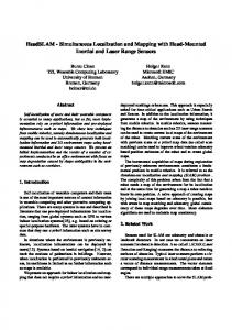
(b) Fig. 2. (a) Sensor beam, showing Flea camera (right) and 3DM-G IMU (center). The beam is 40 cm long. (b) Our planar camera calibration target. Each target square is 104 mm on a side. There are 48 interior corner points, which we use as landmarks. The small red circles in the figure identify the four points whose directions we ‘lock down’ for the self-calibration experiments described in Section V-B.

variance along the camera ray into 3-D, yielding a covariance ellipsoid in the world frame. As a last step, we select three or four highly salient and widely dispersed landmarks as anchors to fix the orientation of the world frame. The covariance ellipsoids for these points are initialized using very small image plane uncertainties. This effectively locks down the initial camera pose and ensures that the full system state is observable.

(42) (43)

For target-free calibration, the initialization procedure is the same as that above, except that the initial camera position is set as the origin of the world frame, and the initial camera orientation is chosen arbitrarily. The camera pose has zero initial uncertainty in this case. As part of the target-free procedure, we estimate the map state (landmark positions in the world frame) as well as the sensor state. We typically select approximately 40 to 60 landmarks as static references for calibration. The positions of the n landmarks in the world frame are initially estimated as: T −1 ui vi 1 , i = 1, . . . , n pW (44) li = d K

E. Feature Detection and Matching We use different feature detection and matching techniques for target-based and target-free calibration. For the targetbased case, we first locate candidate points on the target using a fast template matching algorithm. This is followed by a homography-based check to ensure that all points lie on a planar surface. Once we have coarse estimates of the locations of the corner points, we refine those estimates to subpixel accuracy using a saddle point detector [28]. Target-free calibration is normally performed in a previously unseen and unknown environment. For this case, we select a set well-localized point features as landmarks, using a feature selection algorithm such as SIFT [29]. Feature matching between camera frames is performed by comparing the descriptors for all points that lie within a bounded image region. The size of the search region is determined based on

assuming that the initial direction cosine matrix that defines the camera orientation is the identity matrix. The value d is a nominal landmark depth, while K−1 is the inverse T of the camera intrinsic calibration matrix and ui vi is the vector of observed image coordinates for landmark i. The covariance matrix for each landmark is computed by propagating the image plane uncertainty and a large initial 365

CIRA 2009, Korea, December 15-18, 2009 TABLE I R ESULTS FOR TARGET- BASED CALIBRATION AND TARGET- FREE SELF - CALIBRATION , USING DATA FROM THE SAME EXPERIMENTAL TRIAL . T HE INITIAL HAND - MEASURED (HM) ESTIMATE OF THE CAMERA -IMU TRANSFORM (x, y, z TRANSLATION AND ROLL , PITCH , YAW ORIENTATION ) AND THE FINAL TARGET- BASED

(TB) AND TARGET- FREE (TF) ESTIMATES ARE LISTED , ALONG WITH THEIR RESPECTIVE 3σ ERROR BOUNDS . pz ± 3σ (cm)

Roll ± 3σ (◦ )

Pitch ± 3σ (◦ )

Yaw ± 3σ (◦ )

-15.00 ± 15.00

0.00 ± 6.00

90.00 ± 15.00

0.00 ± 15.00

90.00 ± 15.00

-14.52 ± 0.43

-1.55 ± 0.44

90.59 ± 0.08

0.80 ± 0.09

89.35 ± 0.08

-14.55 ± 0.43

-1.83 ± 0.44

90.56 ± 0.08

0.80 ± 0.09

89.29 ± 0.08

px ± 3σ (cm)

py ± 3σ (cm)

HM

0.00 ± 12.00

TB

6.32 ± 0.54

TF

6.55 ± 0.54

the integrated IMU measurements over the interval between the camera image updates.

B. Experimental Procedure At the start of each experiment, we initialized the filter biases by holding the sensor beam still for approximately 10 seconds. After this settling time, we moved the beam manually through a series of rotation and translation maneuvers, at distances between approximately 1.0 m and 2.5 m from the calibration target. We attempted to keep the target approximately within the camera’s field of view throughout the duration of the trial. Image processing and filtering were performed offline. The camera-IMU transform parameters were initialized using hand measurements of the relative pose of the sensors. We used a subset of 25 images acquired during the cameraIMU procedure to calibrate the camera intrinsic and distortion parameters. Each image measurement was assumed to be corrupted by independent white Gaussian noise with a standard deviation of 2.0 pixels along the u and v image axes. Self-calibration requires us to first lock down the orientation of the world reference frame by fixing the directions to three or more points on the image plane. For our experiments, we chose to fix the directions to the upper and lower left and right corner points on the target (as shown in Figure 2(b)). To do so, we computed the covariance ellipsoids for the corresponding landmarks using very small image plane uncertainties (1 × 10−4 pixels), after averaging the image coordinates over 450 frames (30 seconds) to reduce noise. This averaging was performed using images acquired while the sensor beam was stationary, before the start of an experimental trial. We chose an initial depth of 3.0 m for each of the 48 points on the target, along the corresponding camera ray, with a standard deviation of 0.75 m. It is important to emphasize that the self-calibration algorithm does not require a calibration target. We use the target here for both cases only to evaluate their relative accuracy, with ground truth available.

V. E XPERIMENTS We performed a series of experiments to quantify the accuracy and performance of the target-based and the target-free calibration algorithms. Although we have tested target-free self-calibration in a variety of unstructured environments, in this paper we restrict ourselves to a comparison of the two approaches using the same dataset (images a planar calibration target). The calibration target provides known ground truth against which we can evaluate the quality of the structure recovered by the target-free algorithm. A. Platform We use a black and white Flea FireWire camera from Point Grey Research (640×480 pixel resolution), mated to a 4 mm Navitar lens (58◦ horizontal FOV, 45◦ vertical FOV). Images are captured at a rate of 15 Hz. Our IMU is a MEMS-based 3DM-G unit, manufactured by Microstrain, which provides three-axis angular rate and linear acceleration measurements at approximately 60 Hz. Both sensors are securely bolted to a rigid 40 cm long 8020 aluminum beam, as shown in Figure 2 (a). Our planar calibration target, shown in Figure 2 (b), is 100 cm × 80 cm in size and has 48 interior corner points.

−1

z (m)

−0.5 0 0.5

VI. R ESULTS AND D ISCUSSION

1 −1.5

We compared the target-based and the target-free selfcalibration algorithms using a dataset consisting of 12,046 IMU measurements (6-DOF angular rates and linear accelerations) and 2,966 camera images, acquired over 200 seconds. The calibration target was not completely visible in 20 of the image frames – we simply discarded these frames, leaving 2,946 images for use by the estimation algorithm (in which all 48 target points were successfully identified).

0

−1

−0.5

−0.5

−1

0 −1.5

0.5 −2

1 y (m)

1.5

−2.5

x (m)

Fig. 3. Path of IMU in the world frame over the first 40 seconds of the calibration experiment. The green circle indicates the starting position.

366

CIRA 2009, Korea, December 15-18, 2009 95 Roll (deg)

px (m)

0.1

0

−0.1 0

85 50

100

150

200

Pitch (deg)

py (m)

0

50

100

150

200

0

50

100

150

200

0

50

100 Time (s)

150

200

5

−0.05

−0.15

−0.25 0

50

100

150

0

−5

200

95 Yaw (deg)

0.1 pz (m)

90

0

−0.1 0

50

100 Time (s)

150

90

85

200

(a)

(b)

Fig. 4. (a) Evolution of the IMU-to-camera translation estimate over the calibration time interval (along the x, y and z axes of the IMU frame, from top to bottom) for the target-based calibration procedure. (b) Evolution of the IMU-to-camera orientation estimate (for the roll, pitch and yaw Euler angles that define the orientation of the camera frame relative to the IMU frame, from top to bottom) for the target-based procedure.

95 Roll (deg)

px (m)

0.1

0

−0.1

0

50

100

150

85

200

−0.15

0

50

100

150

100

150

200

0

50

100

150

200

0

50

100 Time (s)

150

200

95 Yaw (deg)

pz (m)

50

0

−5

200

0.1

0

−0.1

0

5 Pitch (deg)

py (m)

−0.05

−0.25

90

0

50

100 Time (s)

150

90

85

200

(a)

(b)

Fig. 5. (a) Evolution of the IMU-to-camera translation estimate over the calibration time interval (along the x, y and z axes of the IMU frame, from top to bottom) for the target-free self-calibration procedure. (b) Evolution of the IMU-to-camera orientation estimate (for the roll, pitch and yaw Euler angles that define the orientation of the camera frame relative to the IMU frame, from top to bottom) for the target-free self-calibration procedure.

The maximum rotation rate of the IMU was 188◦ /s, and the maximum linear acceleration (after accounting for gravity) was 6.14 m/s2 . Figure 3 shows the estimated path of the IMU over the first 40 seconds of the experiment. Table I lists the initial hand-measured (HM) camera-IMU relative pose estimate and the final target-based (TB) and target-free (TF) relative pose estimates. The corresponding plots for the time-evolution of the system state are shown in Figures 4 and 5, respectively. Note that the results are almost identical, and that the target-based relative pose values all lie well within the 3σ bounds of the self-calibrated relative pose values. As ground truth measurements of the relative pose parameters were not available, we instead evaluated the residual pixel reprojection errors for the hand-measured, target-based and self-calibrated relative pose estimates. We determined these residuals by running the UKF using the respective

pose parameters (listed in Table I), without estimating the parameters in the filter. For our hand-measured estimate, the RMS residual error was 4.11 pixels; for the target-based estimate, the RMS residual was 2.23 pixels; for the targetfree estimate, the RMS residual was 2.26 pixels. Both the target-based and target-free RMS residuals are much lower than the hand-measured value, indicating that calibration significantly improves motion estimates. Also, the difference in the magnitude of the residuals increases as the camera frame rate is reduced (below 15 Hz). To evaluate our ability to accurately estimate the landmark positions during self-calibration (i.e. to implement SLAM), we performed a nonlinear least-squares fit of the final landmark position estimates to the ground truth values (based on our manufacturing specifications for the planar target). The RMS error between the true and estimated positions was only 5.7 mm over all 48 target points, and the majority 367


of this error was along the depth direction. This result clearly demonstrates that it is possible to accurately calibrate the camera-IMU transform and to simultaneously determine scene structure in unknown environments and without any additional apparatus. It is perhaps more impressive that this level of accuracy can be obtained with a sensor such as the 3DM-G, which uses automotive-grade MEMS accelerometers and can be purchased for less than $1000 US.

[10] E. M. Foxlin, “Generalized Architecture for Simultaneous Localization, Auto-Calibration, and Map-Building,” in Proc. IEEE/RSJ Int’l Conf. Intelligent Robots and Systems (IROS’02), vol. 1, Lausanne, Switzerland, Oct. 2002, pp. 527–533. [11] G. Conte, C. H. Moog, and A. M. Perdon, Algebraic Methods for Nonlinear Control Systems, 2nd ed. Springer, Dec. 2006. [12] T. S. Lee, K. P. Dunn, and C. B. Chang, “On the Observability and Unbiased Estimation of Nonlinear Systems,” in System Modeling and Optimization: Proc. 10th IFIP Conf., ser. Lecture Notes in Control and Information Sciences. Springer, 1982, vol. 38/1982, pp. 258–266. [13] F. M. Mirzaei and S. I. Roumeliotis, “IMU-Camera Calibration: Observability Analysis,” University of Minnesota, Minneapolis, USA, Tech. Rep. TR-2007-001, Aug. 2007. [14] J. Kelly, “On the Observability and Self-Calibration of Visual-Inertial Navigation Systems,” University of Southern California, Los Angeles, USA, Tech. Rep. CRES-08-005, Nov. 2008. [15] R. Hermann and A. J. Krener, “Nonlinear Controllability and Observability,” IEEE Trans. Automatic Control, vol. AC-22, no. 5, pp. 728–740, Oct. 1977. [16] A. Chiuso, P. Favaro, H. Jin, and S. Soatto, “Structure from Motion Causally Integrated Over Time,” IEEE Trans. Pattern Analysis and Machine Intelligence, vol. 24, no. 4, pp. 523–535, Apr. 2002. [17] J. C. K. Chou, “Quaternion Kinematic and Dynamic Differential Equations,” IEEE Trans. Robotics and Automation, vol. 8, no. 1, pp. 53–64, Feb. 1992. [18] J. M. M. Montiel, J. Civera, and A. J. Davison, “Unified Inverse Depth Parametrization for Monocular SLAM,” in Proc. Robotics: Science and Systems (RSS’06), Philadelphia, USA, Aug. 2006. [19] A. B. Chatfield, Fundamentals of High Accuracy Inertial Navigation, ser. Progress in Astronautics and Aeronautics, P. Zarchan, Ed. American Institute of Aeronautics and Astronautics, Sept. 1997, vol. 174. [20] R. M. Haralick, H. Joo, C.-N. Lee, X. Zhuang, V. G. Vaidya, and M. B. Kim, “Pose Estimation from Corresponding Point Data,” IEEE Trans. Systems, Man and Cybernetics, vol. 19, no. 6, pp. 1426–1446, Nov./Dec. 1989. [21] Y. Ma, S. Soatto, J. Ko˘secká, and S. Sastry, An Invitation to 3-D Vision: From Images to Geometric Models, 1st ed., ser. Interdisciplinary Applied Mathematics. Springer, Nov. 2004, vol. 26. [22] S. J. Julier and J. K. Uhlmann, “Unscented Filtering and Nonlinear Estimation,” Proceedings of the IEEE, vol. 92, no. 3, pp. 401–422, Mar. 2004. [23] S. J. Julier, “The Scaled Unscented Transform,” in Proc. IEEE American Control Conf. (ACC’02), vol. 6, Anchorage, USA, May 2002, pp. 4555–4559. [24] G. H. Golub and C. F. V. Loan, Matrix Computations, 3rd ed., ser. Johns Hopkins Studies in Mathematical Sciences. The Johns Hopkins University Press, Oct. 1996. [25] S. J. Julier and J. J. L. Jr., “On Kalman Filtering With Nonlinear Equality Constraints,” IEEE Trans. Signal Processing, vol. 55, no. 6, pp. 2774–2784, June 2007. [26] J. L. Crassidis and F. L. Markely, “Unscented Filtering for Spacecraft Attitude Estimation,” in Proc. AIAA Guidance, Navigation and Control Conf. (GN&C’03), no. AIAA-2003-5484, Austin, USA, Aug. 2003. [27] B. K. P. Horn, “Closed-form solution of absolute orientation using unit quaternions,” J. the Optical Society of America A, vol. 4, no. 4, pp. 629–642, Apr. 1987. [28] L. Lucchese and S. K. Mitra, “Using Saddle Points for Subpixel Feature Detection in Camera Calibration Targets,” in Proc. Asia-Pacific Conf. Circuits and Systems (APCCAS’02), vol. 2, Singapore, Dec. 2002, pp. 191–195. [29] D. G. Lowe, “Distinctive Image Features from Scale-Invariant Keypoints,” Int’l J. Computer Vision, vol. 2, no. 60, pp. 91–110, Nov. 2004.

VII. C ONCLUSIONS AND O NGOING W ORK In this paper, we presented an online localization, mapping and relative pose calibration algorithm for visual and inertial sensors. Our results show that it is possible to accurately calibrate the sensor-to-sensor transform without using a known calibration target or other calibration object. This work is a step towards building power-up-and-go robotic systems that are able to self-calibrate in the field, during normal operation. We are currently working to deploy our visual-inertial calibration system on several platforms, including an unmanned aerial vehicle and a humanoid robot. Additionally, we are exploring the possibility of using a similar framework to calibrate the transform between different types of sensors, including laser range finders and GPS units. R EFERENCES [1] D. Strelow and S. Singh, “Online Motion Estimation from Visual and Inertial Measurements,” in Proc. 1st Workshop on Integration of Vision and Inertial Sensors (INERVIS’03), Coimbra, Portugal, June 2003. [2] J. Kelly, S. Saripalli, and G. S. Sukhatme, “Combined Visual and Inertial Navigation for an Unmanned Aerial Vehicle,” in Field and Service Robotics: Results of the 6th Int’l Conf. (FSR’07), ser. Springer Tracts in Advanced Robotics, C. Laugier and R. Siegwart, Eds. Berlin, Germany: Springer, June 2008, vol. 42/2008, pp. 255–264. [3] A. I. Mourikis and S. I. Roumeliotis, “A Multi-State Constraint Kalman Filter for Vision-aided Inertial Navigation,” in Proc. IEEE Int’l Conf. Robotics and Automation (ICRA’07), Rome, Italy, Apr. 2007, pp. 3565–3572. [4] J. Kelly and G. S. Sukhatme, “Fast Relative Pose Calibration for Visual and Inertial Sensors,” in Proc. 11th IFRR Int’l Symp. Experimental Robotics (ISER’08), Athens, Greece, July 2008. [5] P. Lang and A. Pinz, “Calibration of Hybrid Vision / Inertial Tracking Systems,” in Proc. 2nd Workshop on Integration of Vision and Inertial Sensors (INERVIS’05), Barcelona, Spain, Apr. 2005. [6] J. Lobo and J. Dias, “Relative Pose Calibration Between Visual and Inertial Sensors,” Int’l J. Robotics Research, vol. 26, no. 6, pp. 561– 575, June 2007. [7] F. M. Mirzaei and S. I. Roumeliotis, “A Kalman Filter-Based Algorithm for IMU-Camera Calibration: Observability Analysis and Performance Evaluation,” IEEE Trans. Robotics, vol. 24, no. 5, pp. 1143–1156, Oct. 2008. [8] J. D. Hol, T. B. Schon, and F. Gustafsson, “Relative Pose Calibration of a Spherical Camera and an IMU,” in Proc. 7th IEEE/ACM Int’l Symp. Mixed and Augmented Reality (ISMAR’08), Cambridge, United Kingdom, Sept. 2008, pp. 21–24. [9] E. Jones, A. Vedaldi, and S. Soatto, “Inertial Structure From Motion with Autocalibration,” in Proc. IEEE Int’l Conf. Computer Vision Workshop on Dynamical Vision, Rio de Janeiro, Brazil, Oct. 2007.

368