pipes linked to a Plexiglas® test section. Two independent ... For the higher flowrates (15 to 125 m3/h), a KrohneTM ultrasonic volumic flowmeter is installed.
EXPERIMENTAL INVESTIGATION OF STRATIFICATION PHENOMENA IN HORIZONTAL TWO-PHASE FLOWS FOR CFD VALIDATION Muriel Marchand, Manon Bottin, Jean-Pierre Berlandis, Eric Hervieu CEA Grenoble DTN/SE2T/LIEX 38054 GRENOBLE CEDEX 9 Abstract The experiment METERO is designed by the French Atomic Energy commission to provide data necessary for the validation of two-phase-CFD simulations in adiabatic conditions. The horizontal test section, equipped with several measurement techniques, allows the exploration of different water/air flow regimes (including bubbly, stratified and transition from bubbly to stratified flow). Measurements of the axial and radial components of the water instantaneous velocity have been carried out using hot film anemometry to characterise the water single-phase flow development. The mean velocity, the fluctuation r.m.s and the turbulent kinetic energy have been inferred. The first results exhibit a good agreement with the literature on turbulent pipe flows. The second campaign is devoted to the study of the bubbly flow configuration for various air mass flowrates. Local void fraction, interfacial area concentration and interface velocity measurements are also performed, using home-made optical probes. After a definition of the needs for CFD validation, the experiments and the measurements techniques are presented and the first test results are shown. The uncertainty associated with the measurement techniques is also discussed.
1. INTRODUCTION The French Atomic Energy commission (CEA) designs, develops and validates simulation tools to calculate the behaviour of multiphase flows in nuclear plants, in incidental and accidental situations. For pressurized water reactors, this topic constitutes a major R&D axis, in the way that the improvement of the simulation tools predictions will lead to a reduction of the uncertainties linked to safety margin. In this framework, the so-called NEPTUNE software platform project, developed jointly by EDF and CEA associated with Areva Nuclear Power (Areva NP) and the French Institute for Nuclear Safety (IRSN), was initiated in 2001 and the experiment METERO, specifically designed for the study of horizontal two-phase flows, was inaugurated in 2006. In horizontal pipes, the evolution of a bubbly flow results from the competition between opponent hydrodynamic mechanisms. On one hand, the turbulence of the main liquid flow is responsible for bubble dispersion and also affects bubble break up and coalescence. On the other hand, gravity effects tend to separate the two phases: when rising up, the bubbles merge and coalesce. Consequently, depending on the relative magnitude of these two phenomena, the flow becomes stratified or not. Compared to many previous experimental programs in horizontal pipes, the METERO experiment is designed to provide all the data necessary for two-phase-CFD simulations. Specially, the two-phase model developed for the CFD scale module of NEPTUNE (Morel et al., 2004, Morel et al., 2005) is devoted to the prediction of two-phase flow in reactor components and needs further experimental validation in adiabatic conditions. The aim of the METERO data is to provide a validation basis of turbulence modelling in bubbly flow and of the dispersion force model. METERO will also constitute a basic test case for the most complex local interface configuration where a “large interface” such as a free surface coexists with the “small interfaces” of the bubbles. This topic remains a challenge for CFD tools.
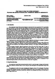
2. EXPERIMENTAL SETUP 2.1 Experiment A front view of the test section is represented in Fig 1. The experiment is constituted of stainless steel pipes linked to a Plexiglas test section. Two independent supply circuits of air and water merge together upstream of the test section by means of an injection/tranquilization system. This system
provides an horizontal bubbly flow at the inlet of the test section. At the test section outlet, water and air are separated in a 1500 litres storage tank. The water temperature is kept constant (around 18° C) by using a heat exchanger in the tank. The main characteristics of the installation are summarized in Table 1. Table 1: Main working parameters of the METERO experiment o o o o o o o
Inlet temperature air-water Maximum outlet temperature Maximum pressure Water flow rate Water velocity Air mass flow rate1 Air superficial velocity
18°C 20°C 2.8 bar 0 to 125 m3/h. 0 to 5 m/s 0 to 350 Nl/mn 0 to 0.7 m/s
Concerning water supply, the circuit is composed by a non pressurized 1500 litres tank and a FinderTM pump, of driving pressure 2.8 bars, maximum flowrate 125 m3/h (which corresponds to a maximum water velocity of 5 m/s) and maximum electric power 18.5 kW, linked to the test section by means of two lines including a flowmeter, a 1 inch line for the scale 0 to 15 m3/h and a 4 inches line for the scale 15 to 125 m3/h. For the small scale (0-15 m3/h), a YokogawaTM Coriolis mass flowmeter is used (accuracy about 0.2 % of the measurement point). For the higher flowrates (15 to 125 m3/h), a KrohneTM ultrasonic volumic flowmeter is installed. It offers a lower accuracy than the Coriolis flowmeter but generates also reduced pressure drop. The inlet water temperature is measured by a type K standard thermocouple with a +/-0.5°C measurement accuracy. This accuracy revealed inadequate for hot film anemometry, very sensitive to flow temperature variations. The thermocouple was then calibrated using a calibration bath and a platinum PT100 sensor.
Fig. 1: Side-view of the experiment Concerning the air supply, it is composed of a 6 bar pressure supply line involving a depressurization/filtration system (the air is depressurized to 3 bar) and two lines of regulation and measurement of the mass flowrate: one line for the range 0 to 50 Nl/mn and a second line for the range 50 to 1000 Nl/mn (not used over 350 Nl/mn, corresponding to a maximum gas velocity of 0.7 m/s ). The air circuit is open: after being separated from the water in the tank, the air is rejected to the atmosphere. The two flowmeters are Brooks EmersonTM thermal massic flowmeters (their accuracy is 0.7 % of the measurement point). They include a PID regulation system that provides very stable inlet conditions and easy use. The air temperature is measured by a type K thermocouple, not calibrated, with a measurement accuracy of +/-0.5°C.
1
The normal conditions, symbolized by the N letter, are taken at 0°C and the atmospheric pressure
The inlet and outlet pressures are measured by means of two KellerTM high precision membrane sensors. They measure the pressure relative to the atmosphere in the range 0-3 bar with an accuracy of +/- 0.015% of the full scale, i.e. +/- 0.45 mbar. The test section, 5.40 m in length, has an internal diameter of 0.1 m. It is composed of interchangeable pieces including instrumentation modules. The inlet injection/tranquilization system is made of 320 tubes for the water and 37 for the air. The number and dimensions of the tubes have been set by iterative tests. The air bubbles injection is made uniformly in the inlet section. The void fraction, directly depending on the number of bubbles injected, is modified by varying the air mass flowrate. The injection system also offers the possibility to choke up some tubes in order to provide a local injection. The system also includes a series of grids designed to break remaining vortices generated by upstream elbows and then ensure a low turbulence level -the so-called grid turbulence- at the inlet of the test section.
Fig. 2: Injection/tranquilization system All the flow parameters can be controlled and/or acquired directly from the control/command room, via a personal computer and use of LabviewTM programs. These programs also ensure the instrumentation data acquisition.
2.2 Instrumentation Several experimental techniques are implemented to investigate the relevant parameters of the flow. Among them, X-ray tomography and resistive wire probes will be used in a near future to provide void fraction maps or the liquid phase height for various sections. The two measurement means already used on the installation and presented herein are hot films and optical probes.
2.2.1
Hot film velocimetry
Hot wire and hot film anemometry have been extensively used in single phase flows for the 50 last years and also adapted for two-phase flows. For our purpose, we use two components DantecTM hot film probes composed of a nickel sensor electrically insulated from the water by a quartz coating. The probes are connected to a constant temperature anemometer (DantecTM CTA Streamline) involving two Wheatstone bridges. The output voltage signals give access to the flow velocity components. An electrode system connected to the ground reference of the CTA is added to the probe so as to protect the films from electrostatic discharges that may destroy the quartz coating and burn the sensors. A filtration system is also used downstream of the pump to retain the particles of size greater than 5 µm. Indeed, the entrainment of those particles by the main flow at high speeds (several m/s) may also damage the coating, reducing the sensor protection. Finally, the response of the CTA Wheatstone
bridge servo-amplifier is adapted to provide the best compromise between high amplification values that give a good frequency response of the measuring system but amplifies instabilities and low amplification values, giving a lower frequency response but damping the parasite oscillations. The resulting overall frequency response (from the sensor to the bridge) is about 7 kHz, which is quite sufficient for our study. The signal is filtered in low pass mode at a frequency of 10 kHz and sampled at 20 kHz. For single phase flow configurations, 200.000 points are acquired, corresponding to 10 seconds. In two phase flow configurations, this duration is increased to 5 minutes. The adjustment of the bridge parameters is made by means of the Dantec StreamwareTM software and the data acquisition is made using a LabviewTM Virtual Instrument. The probe can be moved by a MicrocontrôleTM traversing system so as to measure velocity profiles on test section diametral chord with a 1 mm to 2.5 mm step. The water temperature proved to have a predominant influence on the bridge voltage output. This phenomenon is linked both to the low values used for the probe heating coefficient in water and to the large values of the heat transfer coefficient generated by water convection around the probe. For that reason a heat exchanger installed in the water tank contributes to keep the flow temperature around a constant value (18°). A variation of +/- 0.5° C is authorized around the set point and the voltages are corrected before applying the calibration, using the classical following formula:
T − Ta e(Ta ) ≈ w T −T ref w
0.5
⋅ e(Tref )
(1)
where Ta is the real fluid temperature during the measurement, Tref is the reference temperature and Tw the temperature of the heated sensor. e(Ta) is the film voltage when it is immerged into the fluid at temperature Ta, and e(Tref) is its voltage when it is in the fluid at temperature Tref. The probe calibration is done in situ for various water flowrates, the probe being placed at the center of the test section where the flow velocity is maximum. The relation between the mean and the maximum axial velocity is derived from Schlichting (1955). This procedure implies that the velocity profile follows the classical turbulent 1/n law and also that the flow vertical component can be considered negligible. Its gives for each film the coefficients a and b of the King’s law e2=a Un+b. Concerning the value of the exponent n, literature gives values ranging from 0.45 to 0.5 for hot wire anemometry in air and for values of the Reynolds number based on the probe diameter ranging from 0.02 to 44 Comte-Bellot, Corrsin (1966). Outside these operating conditions, important variations of n have been observed. In our case, the Reynolds numbers based on the probe diameter (70 µm) are around 200, out of the validity range of (Comte-Bellot, Corrsin, 1966). So, the value n has not been imposed but adjusted to get the best fitting of the plot e2=f(Un). If not mentioned, a value n=0.15 is used. Velocity profiles are then acquired, integrated and compared with the water flowrate measured by the flowmeter, for high and low Reynolds number values. This procedure validates the assumptions made for the calibration. In single phase flows, the probe calibration gives access to the axial and radial component of the water instantaneous velocity. A statistical calculation then delivers mean velocity, r.m.s of the velocity fluctuations or kinetic energy profiles. All these operations are realized by LabviewTM. In two-phase flows portions of the signal, a complementary LabviewTM program, named HFA, is used to discriminate the liquid and gas phases. In practise, the appearance of bubbles generates large negative peaks on the voltage signal, as the heat transfer between the probe and the fluid drops when the sensor is in a gas medium. The principle of the HFA program is to cut out the peaks and keep the signal corresponding to the water velocity. The present results will focus only on single-phase flow experiments.
2.2.2
Optical probes
Optical probes, manufactured in the laboratory, are used to measure the temporal phase indicator function in two-phase flows. The principle is to emit a laser signal at the tip of an optical fibre by means of an emission/reception box. The air refraction index leads to a total reflection of the signal, whereas the water refraction index induces a refraction of the signal outside the optical fibre. A photodetector translates this phenomenon into an electrical signal composed of a succession of high
levels (fibre tip in air, corresponding to the transit of bubbles when the sensor is placed into a twophase flow) and low levels (fibre tip in water). This electrical signal is then amplified and a double threshold is applied. The resulting binary signal is the PIF (phase indicator function), acquired to the PC card via the USB port a at 20MHz sampling frequency. The temporal resolution of the measurement is then very high (50 ns). The time average of the PIF gives access to the local void fraction of the flow (α, in %), that describes locally the phases proportion. In our optical probe configuration, a second fibre is placed downstream of the main fibre, at a known distance. The time delay between the two PIFs provides precious information about the interface velocity or the interface area concentration. The overall interfacial area concentration (ai, in m-1) is defined as the total surface area of the interface per unit volume in a finite control volume and represents the geometrical capability of the interfacial transfer. Finally, the mean Sauter diameter is derived from the expression 6α (2) D sm = ai and directly equals the bubble diameter in the case of spherical bubbles. For a non-spherical bubble shape, it gives an order of magnitude of the bubble volume to area ratio. The acquisition of the PIFs and the calculations of void fraction and all other quantities are made via a LabviewTM program named ISO and developed in the laboratory. Concerning the spatial resolution, the typical size of our probes is 250µm for the fibre diameter and several microns for its tip. The two fibres spacing can be reduced to 100 to 200 µm and the axial distance between the front fibre and the rear one is about 500 microns. The probe is mounted in a probe support that is moved by a traverse system in the same manner as for the hot film probes. One can then plot void fraction or interfacial area concentration profiles on a pipe vertical diameter and for different axial locations. The acquisitions are realized on 20000 bubbles for each fibre in order to ensure a good statistical convergence. This corresponds to several seconds in the regions of high void fraction (typically at the top of the test section) but can exceed several tens of minutes in the zones where the flow is quasi single-phasic, such as at the bottom of the pipe.
2.3 Experimental configurations As mentioned previously, the instrumentation modules can be placed at different axial locations along the test section to explore the flow regime in various configurations. For that purpose, 3 measurement sections have been defined for the data collection. The first one is located at X=535 mm downstream the injectors, corresponding to 5 pipe diameters. This location is chosen to characterize properly the inlet conditions. The second one is at X=2040 mm, i.e. 20 pipe diameters downstream the injectors and the last one (X=4050 mm, 40 diameters) is located close to the test section outlet, in the pipe flow fully developed regime. Two data collection campaigns have been defined: the first one with only water to characterize the pipe single-phase flow for two values of the Reynolds number based on the pipe diameter (ReD =1.105 and 3.2 105), corresponding respectively to water flowrates of 30 and 90 m3/h. Measurements of the axial and vertical instantaneous velocity components were performed on a vertical diameter for the 3 locations cited above. The second campaign is devoted to the exploration of the two-phase dispersed flow regime that corresponds to a 125 m3/h water flowrate and various air mass flowrates (ranging from 4 to 30 l/mn). For the 3 sections defined (5D, 20D and 40D) measurements of void fraction profiles were made using a double optical probe.
3. RESULTS 3.1 Single-phase flow set of experiments 3.1.1
Profiles
A first hot film velocimetry campaign was made in the initial configuration for the injection/tranquilization system and revealed the strong influence of the upstream conditions: vortices generated in the different elbows, wake of the injectors…). As mentioned before, a series of corrective
actions were made to ensure a flat velocity profile and low turbulence level at the test section inlet. In Fig. 3 one can appreciate the difference between the mean axial velocity profile U nondimensionalized by the mean flow velocity outside the boundary layer Ue and measured at X=535 mm before (orange) and after (blue) changing the system for a water flowrate equal to 90 m3/h, and ReD =3.2.105. Especially at high Reynolds number values, the impact of the supplementary grids is to reduce the fluctuations due to the wake of the injectors and the overspeed in the highest part of the pipe. The boundary layer thickness is also reduced (about 10 mm compared to 20 mm before). At X=4050 mm, the differences vanish, except for a slight discrepancy in the upper part of the curves. This better agreement is due to the fact that the influence of the upstream conditions is decaying as the flow runs downstream. See for example Fig. 4 showing the comparison at 90 m3/h. 93 83 73
U/Ue U/Ue with grids
y(mm)
63 53 43 33 23 13 3 0
0,2
0,4
0,6
0,8
1
1,2
U/Ue
Fig. 3: Mean axial velocity profiles U/Ue at X=535 mm for ReD =3.2.105 The mean axial velocity exhibits a coherent behaviour with the literature on turbulent pipe flows, with a development of the boundary layers along the X axis. At X=4050 mm the regime is fully developed (jointed boundary layers) in good agreement with literature (Laufer, 1954). At this section, the profile merges satisfactorily with a classical 1/n profile, characteristic of a turbulent flow, with a value n=8 (Schlichting, 1955). Concerning the vertical component, the results show that the profiles are closed to zero whatever the location of the measurement. This is consistent with the fact that the axial component is predominant. Concerning the r.m.s. of the fluctuations divided by the mean velocity Ue outside the boundary layer, one can see in Fig. 5 a series of plots at X=535 mm for the axial component u and in Fig. 6 for the vertical component v both for the two values of the Reynolds number. The comparison between the results before adding the grids (orange and red) and after (blue and green) shows again a thinning of the boundary layers and a better agreement with a low level grid turbulence. The vertical component exhibits the same behaviour. The behaviour of these two quantities is in good agreement with literature on flat plane boundary layers. Indeed, the curvature radius of the pipe can be considered important compared to the scale of the sensor, so the wall of the pipe can be locally assimilated to a flat plane. Anyway, it has to be noted that the threshold values of 0.08 for the axial component and 0.04 for the vertical one are not reached in the near wall region. This is related to the size of the sensor that prevents measurements in the vicinity of the wall. 93
83
73
y(mm)
63
U/Ue with grids U/Ue
53
43
33
23
13
3 0
0,2
0,4
0,6
0,8
1
1,2
U/Ue
Fig. 4: Mean axial velocity profiles at X=4050 mm for ReD =3.2.105
ustd/Ue
0,1 0,09 0,08 0,07 0,06 0,05 0,04 0,03 0,02 0,01 0
30 90 30 90
0
20
40
m3/h with grids m3/h with grids m3/h m3/h
y(mm)
60
80
100
Fig. 5: urms/Ue at X=535 mm for ReD =1.105 and ReD =3.2.105 The same comparison for X=4050 mm is presented in Fig. 7 for urms/Ue and Fig. 8 for vrms/Ue. Globally, the shape of the curves is rather different from the one in the 535 mm location and represents the behaviour of fully developed turbulent profiles. The same remarks can be made concerning the threshold values in the wall nearby region for the same reasons (probe size). Finally, let us notice that the adjunction of grids improved the flow isotropy at X=535 mm. With the new injection/tranquilization system the urms/Ue and vrms/Ue plots merge perfectly, whereas a 30% discrepancy was observed before. This confirms, at the test section inlet, the presence of a homogeneous and isotropic grid turbulence. At X=4050 mm this isotropy is not observed as it is gradually destroyed by the presence of the wall, inducing a high shear. 0,06
30 90 30 90
0,04
m3/h with grids m3/h with grids m3/h m3/h
0,03 0,02 0,01 0 0
10
20
30
40
50
60
70
80
90
100
y (mm)
Fig. 6: vstd/Ue at X=535 mm for ReD =1.105 and ReD =3.2.105 0,1 0,09 0,08 0,07
ustd/Ue
vstd/Ue
0,05
0,06 0,05 0,04
30 m3/h with grids 30 m3/h 90 m3/h with grids 90 m3/h
0,03 0,02 0,01 0 0
10
20
30
40
50
60
70
80
90
100
y(mm)
Fig. 7: ustd/Ue at X=4050 mm for ReD =1.105 and ReD =3.2.105
0,05 0,045 0,04
vstd/Ue
0,035 0,03 0,025
30 m3/h with grids 30 m3/h 90 m3/h with grids 90 m3/h
0,02 0,015 0,01 0,005 0 0
20
40
60
80
100
y(mm)
Fig. 8: vstd/Ue at X=4050 mm for ReD =1.105 and ReD =3.2.105 The turbulent kinetic energy profiles have been plotted using the expression (see for instance Fig. 9 for X=4050 mm and ReD =3.2.105):
k=
(
1 ⋅ u ′2 + 2 ⋅ v′2 2
)
(3)
This relation assumes that the third (orthoradial) component behaviour is similar to the one of the vertical (radial) component. If this assumption is realistic for single-phase flows, it is false for bubbly flows where 3D effects may become predominant. The three velocity components obtained by a 3 component probe or by probe rotation, will then be necessary to infer the turbulent kinetic energy profiles. 0,07
k (m 2/s2)
0,06 0,05 0,04 0,03 0,02 0,01 0 0
20
40
60
80
100
y(mm)
Fig. 9: Turbulent kinetic energy profile at X=4050 mm for ReD =3.2.105
3.1.2
Discussion about the measurement uncertainty
If the uncertainty on the location of the sensor is given by the accuracy of the traverse system (several microns), on the other hand the uncertainty on the instantaneous velocity depends on numerous factors, not always well known (calibration errors, uncertainty on the angle between the sensor and the test section symmetry axis, on the probe yaw factor, on the fluid temperature…). From the uncertainty on the water flowrate Q, given by the constructor,
dQ =0.5 % and the Q
uncertainty on the pipe diameter which has been estimated to 0.1%, one can then infer:
dVdeb dQ dD = + 2⋅ Vdeb Q D where Vdeb is the water mean flowrate velocity and with dVdeb/Vdeb=0.7%.
(4)
The impact of a sensor misalignment with respect to the pipe axis (the angle θ is 45° for film 1 and 45° for film 2) has been tested, by the adjunction of an uncertainty dθ in the programs that infer the velocity from the voltages. A 0.01° error (value given by Dantec) leads to a negligible error on the instantaneous axial component u (less than 0.001%) and a 1.8 % error on the vertical component v. It has to be noticed anyway that this is a systematic error that will affect the mean values but will be eliminated by the calculation of the r.m.s. Concerning the yaw factor ky that represents the sensor sensibility to the tangential component of the velocity, it is very small (about 0.04). Theoretically, its value may change with the probe orientation with respect to the pipe axis, anyway the manufacturor indicates that for this type of probes, this value doesn’t change much. The influence of ky fluctuations has also been tested in the program. The results show that a variation of +/-0.01 (i. e. +/-25%) generates a +/-0.05% error on u and +/0.09% on v. The influence of errors on ky is then very slight. On the contrary, the effective fluid temperature has a huge influence on the measurements. Using equ. (1), one can show that only a 0.1°C error on the water temperature leads to a 2.5 % error on u and 6 % error on v. Finally, if one considers that the different errors are cumulated, the uncertainty on the axial instantaneous velocity u is about 3 % and the uncertainty on the vertical instantaneous velocity v is about 8 %. Anyway, it has to be recalled that the main source of error on v is systematic and then eliminated by the r.m.s. calculation.
3.1.3
Conclusion of the single-phase flow measurements
In conclusion, this first campaign showed that the Metero experiment presents a single-phase pipe flow in good agreement with the literature on the subject. The inlet flow is a grid turbulence one, it then develops to reach a fully developed turbulent pipe flow at the outlet of the test section. The modifications brought to the injection/tranquilization system improved the stability and the isotropy of the flow.
3.2 Two-phase flow set of experiments 3.2.1
Optical probes measurements
As mentioned previously, void fraction measurements were made using a double optical probe at 3 locations and from the PIFs, void fraction (in %), interfacial area concentration (in m-1) and mean Sauter diameter (in m) were inferred. Fig. 10 gives a comparison between the void fraction profiles for X=4050 mm and 4 values of the air mass flowrate from 4 to 30 l/mn. One can easily see that the void fraction rises when going from the lower to the upper wall, and from the low to the high air flowrates. The results are in good agreement with (Iskandrani & Kojasoy, 2001), anyway the void fraction peaks near the upper and lower walls, that these authors measured, are not observed in the present data. This is probably linked to the size, not of the probe itself, but of the probe support, 6 mm in diameter, that prevents measurements in the vicinity of the wall. Void fraction (%) 0.16 0.14 0.12
Y(µm)
4 8 12 30
0.1 0.08 0.06 0.04 0.02 0
-1
-0.5
0
0.5
1
Fig. 10: Void fraction profiles at X=4050 mm for Qw=125 m3/h
The same remark can be made for the local interface area concentration (Fig. 11) which is equal to 4 times the ratio between the interface frequency and the interfacial velocity. This relation relies on the assumptions that the bubbles are spherical, that they are homogeneously distributed within the flow and that the flow direction is unidirectional, collinear with the probe prongs. As in our case, the bubble size was very small (from 0.5 to 2 mm in chord) the assumption of spherical bubble shape is quite valid. It was moreover confirmed by fast scan camera acquisitions. It has to be noted that the local interface area concentration is more important at the upper part of the test section and for high values of the air flowrate. This is related to the migration and coalescence of the bubbles. Due to their high density difference with the water, the air bubbles, once emitted in the flow, tend to rise and merge. This results in high void fractions and high interfacial area concentration in this zone. The analysis of the mean Sauter diameter (Fig. 12), that represents roughly the mean bubble diameter, and is calculated by 6 times the ratio between the void fraction and the local interface area concentration, brings more details on the bubble behaviour. The same phenomenon is highlighted but moreover, one can identify 3 zones, distributed in the following manner: A first zone located in the lowest half of the pipe (Y ranging from 100.000 to 50.000 µm), and involving small bubbles of quasi constant diameter for a given value of the air flowrate. This corresponds to a quasi single-phase zone, the gas phase being dispersed and the void fraction being rather low. In this region, the small size of the bubbles and their dispersion slow down coalescence. In a second zone (Y ranging from 15.000 to 50.000 µm), the evolution of the bubble diameter with the altitude is quasi linear. This may correspond to a region of coalescence. The bubble size and the void fraction have reached a threshold value beyond which coalescence is promoted. Then in the upper zone (Y ranging from zero to 15.000 µm), the bubble diameter is high, but rather constant versus Y. This corresponds to a bubble layer, analogous to the mechanical boundary layer, where wall shear effects may prevent the coalescence phenomenon. Interfacial area (m-1) 0
100
200
300
400
500
0 10000 20000
Y(µm)
30000 40000
4 8 12 30
50000 60000 70000 80000 90000 100000
Fig. 11: Interfacial area concentration profiles at X=4050 mm for Qw=125 m3/h Mean Sauter diameter (mm)
0
0.5
1
1.5
2
2.5
0 10000 20000 30000 Y (µm)
40000 50000 60000 70000
4 8 12 30
80000 90000 100000
Fig. 12: Mean Sauter diameter profiles at X=4050 mm for Qw=125 m3/h
Optical probes also give access to the gas velocity, as shown in Fig. 13. Gas velocity (m/s) 0
1
2
3
4
5
6
0 10000 20000
Y (µm)
30000 40000 50000 60000 70000
4 8 12 30
80000 90000 100000
Fig. 13: Gas velocity profiles at X=4050 mm for Qw=125 m3/h As the gas phase is mainly transported by the liquid one in dispersed regime, qualitative comparisons can be made with the work of Inskandrani and Kojasoy (2001) concerning liquid velocity profiles measured in two phase flows. The authors observed that the profiles are non symmetric, the maximum velocity point is shifted to the bottom of the pipe and the profiles exhibit a sharp reduction of the velocity in the vicinity of the top wall. Inskandrani and Kojasoy explained this particular shape by the presence of a bubble layer at the top of the pipe that slows down the flow, especially because of the additional turbulence created. These analogies between gas and liquid velocity profiles confirm that the bubble transport is mainly supported by the liquid motion. A way to check the accuracy of our optical probe measurements is to integrate the product of the gas velocity times the void fraction and to compare it to the gas superficial velocity. The cross section has been virtually cut into several trapezoid shaped areas and the assumption has been made that, in each area, void fraction and gas velocity are constant. These hypotheses are false, especially concerning the gas velocity, but, our objective is mainly to check the consistency of our results. The product of gas velocity times void fraction has then been integrated and compared to gas superficial velocity. The discrepancies are in the range 2-10 %. 3.2.2
Optical probe measurement uncertainty
Void fraction measurement using optical probes is a far less known technique than hot wire or hot film anemometry. Nonetheless, studies have been made to characterise the optical probe measurement accuracy. Among them, one can cite Le Corre (2000). Concerning the uncertainty on the spatial location, as the probe tip is very punctual (several microns), the uncertainty is mainly related to the one of the traverse system, given by MicrocontroleTM to several microns. Comparisons made by Le Corre (2000) with electrical probes showed that the discrepancy on the void fraction measurements can reach 20% and that the probe design is the main influencing factor. Consequently, a special care is taken to reduce the size of the optical fibre tip and the distance between the fibres. For our study, the reproducibility of the results has been tested by carrying out many times the same measurements, in the same conditions. A 4 to 5 % discrepancy was found. Concerning the dependency to fluid temperature, it has been observed a small effect of temperature variation on the measurements. A fluctuation of 5 °C on the water temperature leads to a 10 % variation on the void fraction. This could be partly related to the measurement uncertainty but is nonetheless systematic. It is not linked to the principle of measurement which is independent of temperature but may probably due to the variation of the two fluid physical properties with temperature. For this reason, the optical probe measurements were carried out at a constant temperature of 18°C.
3.2.3
Conclusions of the two-phase flow campaign
The optical probe measurement campaign highlighted a two-phase dispersed flow, in good agreement with literature on the subject. The void fraction profiles show that for a given abscissa of the test section, the void fraction increases with the altitude and the air mass flowrate. For a given altitude, the results also show that the void fraction increases when going downstream, which seems to highlight a coalescence phenomenon. Anyway, measurements at the downstream section (X=4050mm, 40D) did not exhibit stratification, for the highest value of the water flowrate, the flow regime remains dispersed on the whole test section. Interfacial area concentration and mean Sauter diameter profiles are in good agreement with the void fraction ones, bringing more information on the flow.
4. CONCLUSIONS The results presented in this paper concern the single-phase and two-phase flow characterisation on the experiment METERO, by means of hot film anemometry and optical probes. The aim is to build a database for the validation of the NEPTUNE CFD code. The one-phase flow results show an academic flow, in good agreement with the literature on turbulent pipe flows. The modifications brought to the injection/tranquilisation system greatly improved the flow. The two-phase flow campaign by means of optical probes in a dispersed bubble regime is also in good agreement with the literature consulted on the subject. Hot film measurements are also on progress and will bring more information on the flow behaviour.
ACKNOWLEDGMENTS This work has been achieved in the framework of the NEPTUNE project, financially supported by CEA (Commissariat à l’Énergie Atomique), EDF, IRSN (Institut de Radioprotection et de Sûreté Nucléaire) and AREVA-NP.
REFERENCES Comte-Bellot, G., Corrsin, S., 1966, J. Fluid Mech., 25, part 4, 657-682. Iskandrani, A., Kojasoy, G. 2001 Nuclear Engineering and Design 204 117-128. Laufer, J. 1954 « The structure of turbulent velocity in fully developed pipe flow », NACA report 1174. Le Corre, J. M. 2000 “Benchmark and numerical evaluation of multi-sensor instrumentation techniques in two-phase flow”, Thesis of Purdue University. Morel, C., Pouvreau, J., Lavieville, J., Boucker, M. 2004 “Numerical Simulations of a bubbly flow in a sudden expansion with the NEPTUNE code”, 3rd Int. Symposium on two-phase flow modelling and experimentation, Pisa, Italy, September, 22-24. Morel, C., Mimouni, S., Lavieville, J., Boucker, M. 2005 “R113 boiling bubbly flow in an annular geometry simulated with the NEPTUNE code”, 11th International Topical Meeting on Nuclear Reactor Thermal-Hydraulics, Avignon, France, October, 2-6. Schlichting, H. « Boundary layer theory », 1955, Mc Graw Hill.