A Fast Algorithm for Simulated Annealing - McGill Physics

Physica Scripta. Vol. T38,40-44, 1991.

A Fast Algorithm for Simulated Annealing Hong Guo, Martin Zuckermann, R. Harris and Martin Grant Centre for the Physics of Materials, Department of Physics, McGill University, 3600 University Street, Montreal, Quebec, Canada H3A 2T8 Received September 24, 1990; accepted October 26, 1990

Abstract We present a new deterministic algorithm for simulated annealing and demonstrate its applicability with several classical examples: the ground state energies of the 2d and 3d short range king spin glasses, the traveling salesman problem, and pattern recognition in computer vision. Our algorithm is based on a microcanonical Monte Carlo method and is shown to be a powerful tool for the analysis of a variety of problems involving combinatorial optimization. We show that the deterministic method generates optimal solutions faster and often better than the standard Metropolis method.

1. Introduction Over the last two decades extensive analytical and numerical work has been performed in order to obtain approximate solutions to optimization problems involving many parameters and conflicting constraints [ 11. Classic examples of such problems include the traveling salesman problem (TSP), the three dimensional spin glass ground state, and the wiring of gates in chip design. There exists an entire class of these problems which is termed “NP-complete” (non-deterministic polynomial time complete) because the computational effort used to find an exact solution increases exponentially as the total number of degrees of freedom, N , of the problem. This implies that approximation methods are required for further analysis. Indeed, heuristic methods are widely used for such practical optimization problems in computer science and engineering and they prove to be extremely fruitful. However, these methods are usually problem-oriented and their domain of application is restricted to the particular problem which they are designed to solve. As the value of N for a particular problem increases, algorithms based on statistical method become useful, and allow unified treatment of the NP-complete problems. The most successful statistical method to date is the stochastic model of simulated annealing introduced by Kirkpatrick, Gelatt, and Vecchi in 1983 [2]. In simulated annealing, a cost function is constructed to characterize the optimization process and minimization of this function gives an approximation to the optimal solution of the problem. A controlled thermal treatment followed by slow cooling give the system the chance to jump out of local minima of the cost function to improve solutions. Constructing the cost function can in principle be problematic, although in practice the choice is often straightforward. For instance, the distance the salesman travels is the cost function of TSP. Simulated annealing has been applied to the problem of finding the ground state of a spin glass (SG) which is an NP-complete problem in three dimensions [3, 41. A short range Ising spin glass is described by the Hamiltonian where Si = f 1 is the spin at site i of a cubic lattice; Jij is usually assumed to be a random number drawn from a Physica Scripta T38

Gaussian distribution (Gaussian model), or takes values of fJ with equal probability ( fJ model). The sum is over all the nearest neighbor pairs. The spin glass system is highly frustrated and has a large number of metastable states with similar energies. Its ground state also has high degeneracy. At low temperatures it can be trapped in one of the metastable states. Thermal noise then induces uphill steps in energy space which in principle eventually brings the system to equilibrium. The simulated annealing method starts with the system at high temperature and lowers the temperature in small steps according to a prescribed annealing schedule. For a SG, the system energy is used as the cost function. At each temperature, enough simulation steps (spin flip trials) must be performed in order to ensure the system is equilibrated [3, 41. At very low temperature, this process causes the SG system to freeze into a state which is at least an approximation to the true ground state. For other combinational optimization problems, a temperature is also introduced as a control parameter measured in units of the cost function. Usually simulated annealing is performed using the Metropolis [5] algorithm with temperature T fixed at each state of the annealing schedule. The total cost function of the system is lowered due to local ordering and the temperature provides the activation necessary to bring the system out of its metastable states. However, for metastable states with high energy barriers, it is very hard for the thermal noise to provide enough activation. Thus the system can be locked into a local minimum of the cost function space. This is the reason that the annealing schedule must be carefully designed and the annealing steps must be small [3, 41. In this paper we present a study of an algorithm for simulated annealing which directly and deterministically minimizes the cost function. The method is based on a microcanonical ensemble in which the system of interest is in contact with an auxiliary system (a “demon”) and the cost function (energy) is exchanged between both systems. In this method the temperature is actually a derived quantity. This allows large local temperature fluctuations which are essential for bringing the system out of metastable states. The methodology of the microcanonical Monte Carlo was first proposed by Creutz [6] to study the Ising model and has subsequently been applied to a variety of physical systems [7]. Although equilibrium statistical mechanics using the canonical and microcanonical ensembles are equivalent, the dynamics of the algorithms based on these ensembles are different. We find that this microcanonical Monte Carlo method is very naturally applicable to optimization problems because it is deterministic and allows large temperature fluctuations. To our knowledge, an early attempt to use microcanonical Monte Carlo to study low temperature properties of a spinglass was due to Dasgupta, Ma and Hu [8]. Recently, Sourlas

A Fast Algorithm for Simulated Annealing

41

[9] has also applied a microcanonical method to investigate the ergodicity properties of a spin-glass. While the ideas are similar, the algorithm to be presented below is most close to the one proposed by Clover [lo]. In Section 2 we present the method and apply it to several classic problems: the Ising spin glass, the STP and a short discussion on its application to computer vision. Section 3 is reserved for a short summary and conclusion. All of our simulations were performed on a SUN 3/50 workstation.

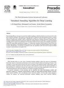
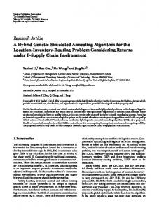
We have applied our method to study both spin glass models. In 2d, the systems were on square lattices with up to 100’ spins. In 3d, cubic lattices with up to 303spins were used. Periodic boundary conditions were used for all simulations. The units of energy were taken as J for the fJ model and 6 J for the Gaussian model. For the 2d Gaussian model, we started with E r = 8 and annealed down to E r = 0 with equal steps of 1. The systems used consisted of 100’ spins, and 400 or 800 Monte Carlo trials per spin were done for each E r . 10 runs were averaged to give the value Eo/GJx - 1.30 f 0.004, which is 2. Method and results in good agreement with that given by the transfer matrix Although the microcanonical Monte Carlo method has been method. Our results also compare favorably with those of the discussed in detail by Creutz [6], we briefly present it here Metropolis algorithm. for completenes. Consider a nearest neighbor Ising model For the 3d Gaussian model, the range of we used was described by Hamiltonian (1) with J,j= J , from 8 down to 0 with steps of 1 for the first 5 stages and 0.5 for the last 5 stages. For lattices with 163spins, 600 Monte Elsing = - J SiS’. (2) Carlo trials per spin were done for each of the Averaging To study its equilibrium properties, a microcanonical ensemble 30 independent runs gave Eo/SJ x - 1.674 f 0.0015 which is constructed by letting a demon with energy Edinteract with is somewhat higher than the transfer matrix estimate, although the spins such that the total energy E = Elsing Ed is con- within the error bars, but considerably lower than that found served. In a Monte Carlo simulation, the energy required to using the Metropolis Monte Carlo [3]. For lattices with 303 flip a spin, 6E, is compared with Ed, and if Ed 2 GE, the flip spins, test runs were also done using the same annealing is permitted and an amount of 6E is subtracted from E d . schedule but with only 300 Monte Carlo trials per spin per Otherwise the trial is abandoned. It is easy to show [6] that the E r , we foundf Eo/6J = - 1.667 after averaging 5 runs. average demon energy measures the temperature of the Ising Since the transfer matrix calculation quoted above is persystem in equilibrium. formed on systems with 43 spins, and there is very little The microcanonical Monte Carlo method is generalized information about the ground state energy for larger systems, for simulated annealing as follows. We begin the simulation our results could provide a benchmark for further simulations. from 16 The 2d & J model was studied by using with the system at a disordered high temperature state and allow it to interact with the demon. At each stage of the down to 0 in steps of 4, with either 800 or 1600 Monte Carlo annealing schedule a maximum value of the demon cost steps per spin for each of the E r on lattices with 50’ spins. function, C Y (e.g., Ed for SG), is specified such that if the Averaging 10 independent configurations gave Eo/J x demon cost function cd > C y , cd is reset to C r . This - 1.401 & 0.004, again in excellent agreement with the procedure brings the system very efficiently to lower and transfer matrix calculation. Test runs on systems with 100’ lower cost function states. For frustrated systems with local spins essentially gave the same result. The Metropolis algorordering, a “hot” demon can melt a local ordered region and ithm gives Eo/J x - 1.3974 while the extrapolation gives bring the system out of metastable state. In the simulations - 1.398 [4]. Our results agree very well with these values. The 3d f J model simulation used the range of E r from reported below, we found that the choice of C y Xwas rather were used for robust: any reasonable choice did equally well. This method 20 down to 0 in steps of 4. A total of 12 Y’S can also be used after a heuristic treatment of the problem. In a run, 600 or 1200 Monte Carlo steps were done for each that case, since the initial state is almost ordered, we start E T X .For lattices of 163 spins, 40 independent runs were with the demon possessing a large value of the cost function averaged to find the value of the ground state energy, E,:J z - 1.773 f 0.001 (we have also performed test runs and then anneal down. on lattices with 303spins; 5 independent runs averaged to give 2.1. Ground state energy of the Zsing spin glass - 1.772). Note that this value is actually lower than that of the transfer matrix calculation, though within its error bars. The short range Ising spin glass described by (1) has been Grest et al. [4] give a value of - 1.7706 using Metropolis extensively studied for many years [l 13. For the fJ model, Monte Carlo, which they extrapolate to - 1.791. transfer matrix calculations [ 121 yield the ground state Figure 1 shows the decrease of energy as a function of time energies: Eo/J x - 1.40 f 0.01 for d = 2, and Eo/J x for the 2d models using the parameters mentioned above. The - 1.76 f 0.02 for d = 3, where d is the dimensionality of the energy decreases continuously until E r is lowered and a system. For the Gaussian model, the transfer matrix method sudden drop of energy occurs. This is more apparent for the [12] gives Eo/6J x - 1.31 f 0.01 for d = 2 and Eo/SJ x f J model because the energy is discrete. Figure 2 compares - 1.7 f0.03 for d = 3, where GJis the width of the Gaussian approaches to the ground state as a function of time using distribution for Jij. Other numerical methods have also been both Creutz and Metropolis Monte Carlo methods for the 2d used to obtain the ground state energies but usually yield values higher than those quoted above, illustrating the diffi- Gaussian model. The same bond configuration (J,’) is used culty of reaching the true ground state. For example, simulated for the two simulations. Grest et al. [4] have shown that the annealing using Metropolis Monte Carlo gives, for the 2d ground state energies obtained by Metropolis Monte Carlo Gaussian spin glass [4], Eo/SJ x - 1.2867. Grest et al. then method depend on the cooling rate, thus we used the same extrapolate to the limit of infinitely slow cooling rate [4] to get parameters which gave the best results in their simulation. AS shown in Fig. 2, our method gives a faster convergence to the a value of - 1.308.

1

r.

+

Physica Scripta T38

Hong Guo et al.

42

1

I+,

I

1 1

models. For the 3dmodels, lower energy states are also found using our method.

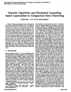
2.2. The traveling salesman problem The TSP has been studied for a long time as the representa......model .......... tive problem for combinatorial optimizations [ 131. The TSP -0.50 tries to find the shortest path connecting N nodes (cities), with h the path ending at its starting node. Since this belongs to the 0 class of NP-complete problems, exact solutions have been attempted only for cases with less than a few hundred nodes. However, simulated annealing has been applied to this -1.00 problem where up to several thousand nodes are present [2]. We have applied our algorithm to TSP. We first consider a system with N = 400 nodes randomly distributed on a *-*-.- ........................ square of linear size f i = 20. The cost function, L, is the length of the path connecting the N nodes. The length is -1.50 " ' ' I ' ' ' ' ' ' 0 2500 SO00 7500 measured in the "Manhattan" metric where the distance between two nodes is the sum of their separations along the time Cartesian coordinates. We number the nodes from 1 to N Fig. 1. Typical runs showing the approach to the ground state of the 2d and a path is represented as a particular permutation of models. Energy is measured in SJ for the Gaussian model and J for the f J { 1 . . . N } . The rearrangements of the path are done using the model. The time is measured in Monte Carlo steps. System sizes are 10O2 for strategy of Lin [14] where moves consist of reversal and the Gaussian model and 5d for the & J model. replacement [ 151. We used an annealing schedule in which the maximum of ground state, in addition to the better values obtained. Our the demon cost function L y starts at f i / 4 and is then results also show little variation of the energy, since in micro- usually lowered in equal steps. At most 45 L y ' s are used in canonical Monte Carlo the total energy is a conserved quantity a simulation. A Monte Carlo step here corresponds to a reconfiguration trial on the path, and we used up to 160000 and Ed has an upper bound. In all of our simulations we found that the choice of erax (400N) Monte Carlo steps for each annealing stage. Howis rather robust. Provided we start with some large value and ever, if there are too many succussful reconfigurations, it goes down with reasonable steps, the final results are not either means L y is too large or the system is too "hot", and significantly affected. Of course, careful design of the anneal- thus we can go to the next annealing stage with a lower value ing schedule could in principle improve the rate of convergence of L y . In our simulation, if 4000 (10N) successful reconto the ground state. The numbers quoted above are for figurations are made, we jump to the next annealing stage typical runs with a natural annealing schedule. Another directly. A typical measure of the TSP solution, denoted by advantage or our algorithm is that no extrapolation [4] is a, is the total path length divided by N . a will be independent needed to get the values for true ground state for the 2d of N if many runs are averaged [16]. For N = 400, and the nodes uniformly distributed, our algorithm gives a sz 0.98 f 0.03 by averaging 10 independent runs. We obtain the same value of a using the standard simulated annealing with Metropolis Monte Carlo, but more than twice the CPU time was needed. When using 40000 (100N) Monte Carlo steps per annealing stage, there is a slight increase in the value of a [17]. -------------____. Figure 3 shows a typical solution where 400 nodes are -0.50 distributed in 9 equal size regions separated by empty space. After 15 stages of annealing, long paths acrossing the regions are infrequent while in each region the paths are still rather disordered (see Fig. 3(a)). Fig. 3b is the result after 45 stages of annealing which gives a = 0.72. Reference [2] gives a -1.00 larger value a = 0.784 for the case where the nodes are arranged similarly to ours, although it should be noted that the difference in the a's are presumably due to the details of the actual configurations.

2

Gaussian model

9

I

-1.50

'

'

2.3. Restoration of corrupted binary images In addition to the two examples discussed above, there are time many other practical problems which can be studied with this Fig. 2. Typical runs using the Creutz and Metropolis Monte Carlo methods algorithm. For example, a large class of computer vision and for the 2d Gaussian model. Energy is measured in SJ. The same bond configurations are used for the two curves. System size is 10O2. For the image interpretation problems can be described and disMetropolis method, the initial temperature is 1.5 and it is lowered in steps cussed within the framework of optimization theory [18, 191. of 0. I . For each temperature, 500 Monte Carlo steps per spin are performed. Forest [20] considered the following cost function for the 0

Physica Scripta T38

4000

8000

A Fast Algorithm for Simulated Annealing

43

is largest at corners), the annealing method has to be supplemented by other heuristics which preserve the corners [ 191. We are currently studying this problem and results will be presented elsewhere.

3. Conclusion t

The main goal of this work has been to introduce a Creutz algorithm for simulated annealing. We found that this method is particularly powerful for problems involving frustration and local ordering. This was demonstrated in the short range Ising spin glass simulations. An obvious merit of the Creutz algorithm is that it is deterministic, so that programs can be made rather efficient. Although an exhaustive investigation of the parameter space was not carried out, we found that other reasonable annealing schedules give essentially the same performance as those presented in the text. This method can therefore provide an efficient approach to optimization problems where no good heuristic method is known. For problems where long range reconfigurations are needed, the performance enhancement of Creutz algorithm over Metropolis algorithm decreases. As mentioned above, we gain only a factor of less than 3 in CPU time for TSP. Improvement in this regard could be achieved by introducing multiple demons into the algorithm, so that at any instant during a simulation, many different demon energies are present to be consulted. A hybrid algorithm of combining the Creutz and Metropolis algorithm could also be useful in some instances. We have also tested another annealing method in which the total cost function, system plus demon, is held constant at each stage of the schedule. The annealing is achieved by systematically lowing the total cost function. Preliminary results show that this method performs as well as the one presented in the text. In conclusion, we have introduced a new algorithm for the simulated annealing of NP-complete problems, and shown that it provides a distinct improvement over previous methods. Fig. 3. (a) A TSP path after 15 stages of annealing starting with LFu = 5 for 400 nodes distributed uniformly in 9 equal size regions: (b) The path after 45 stages of annealing. a = 0.72 for this path.

binary image restoration problem

E =

-.IC $4 -

1/2

1 Di(l + Si) In ( p - ’

- 1)

(3)

where Si = f 1 denotes the binary values of the pixel i, 0,= f 1 are the initial binary values of the same pixel (i.e. D, is the pixel in the corrupted image); and p is the noise strength with a value between 0 and 1. The sum is over the nearest neighbor pairs of pixels. When an image is corrupted by white noise, it can be shown [20], that the configuration { S , ) which minimizes E is an approximation to the original uncorrupted image. The cost function (3) has the same form as a random field Ising model where Di is a space dependent random field. Thus we have applied our method of simulated annealing to determine the global minimum of (3) and fine that the noise is annealed away very efficiently. For an image (a Chinese character) of 50 000 pixels corrupted with noise strengthp = 0.25 (25% of the pixels are corrupted), only 3 % noise is left after 120 trials per pixel (6 annealing stages with 20 trials each). However, since corners of a picture are not preserved by thermal treatment (the probability of flipping

Acknowledgements This work was supported by the Natural Sciences and Engineering Research Council of Canada, and le Fonds pour la Formation de Chercheurs et I’Aide a la Recherche de la Province du Quebec.

References I . Schwefel, H. P., Numerical Optimization of Computer Models, John Wiley and Sons (1981) (Edited by N. Christofides, A. Mingoui, P. Toth and C. Sandi), Combinatorial Optimization London and New York, Wiley-interscience (1979). 2. Kirkpatrick, S.,Gelatt, C. D. and Vecchi, M. P., Science 220, 671 (1983); Kirkpatrick, S., J. Stat. Phys. 34,975 (1984). 3. Soukoulis, C. M., Levin, K. and Grest, G. S., Phys. Rev. B28, 1495 (1983); Reger, J. D., Binder, K. and Kinzel, W., Phys. Rev. B30,4028 ( 1985). 4. Grest, G . S., Soukoulis, C . M. and Levin, K., Phys. Rev. Lett. 56, 1148 (1986). 5. Metropolis, N., Rosenbluth, A., Rosenbluth, M., Teller, A. and Teller, E., J. Chem. Phys. 21, 1087 (1953). 6. Creutz, M., Phys. Rev. Lett. 50, 1411 (1983). 7. Bhanot, G., Creutz, M. and Neuberger, H., Nucl. Phys. B235, 417 (1984); Creutz, M., Gocksch, A., Ogilvie, M. and Okawa, M., Phys. Rev. Lett. 53, 875 (1984); Harris, R., Phys. Lett. 111A, 299 (1985). 8. Dasgupta, C., Ma, S. K. and Hu, C. K., Phys. Rev. B20,3837 (1979). 9. Sourlas, N., Europhys. Lett. 6,. 561 (1988). IO. Clover, M., (unpublished). Physica Scripta T38

44

Hong Guo et al.

and William T. Vetterling, Numerical Recipes. Cambridge University 11. Binder, K. and Young, A. P., Rev. Mod. Phys. 58, 801 (1986) and Press, New York (1987). references therein. 12. Cheung, H. and McMillan, W. L., J. Phys. (London) C16,7027 (1983); 16. Beardwook, J., Halton, J. H. and Hammersley, J. M., Proc. Cambridge Philos. Soc.55, 299 (1959). Morgenstern, I. and Binder, K., Phys. Rev. Lett. 43, 1615 (1979); Z. Phys. B39,227 (1980); Phys. Rev. B22,288 (1980); J. Appl. Phys. 52, 17. Our value of LY is slightly higher than those of Ref. [2] where the simulated annealing is performed after treatment by a heuristic method. 1692 (1981). 13. Dantzig, G. B., Fulkerson, D. R. and Hohnson, S. M., Oper. Res. 2, 18. Buxton, B. F. and Murray, D. W., Image and Vision Computing 3, 163 (1985); Buxton, B. F., Buxton, H. and Kashko, A. in Parallel 393 (1954); Garey, M. R. and Johnson, D. S., Compters and IntracArchitectures and Computer Vision (Edited by Ian Page), Clarendon tability: A Guide to the theory of NP-Completeness, (Freeman, San Press, Oxford (1988). Francisco, 1979). 19. Geman, S. and Geman, D., IEEE Trans. PAM1 5, 721 (1984). 14. Lin, S., Bell Syst. Tech. Jour. 44, 2245 (1965). 15. A FORTRAN program for the traveling salesman problem is provided 20. Forrest, B. M. in Parallel Architectures and Computer Vision (Edited by Ian Page), Clarendon Press, Oxford (1988). in the book of William H. Press, Brian P. Flannery, Saul A. Teukolsky

Physica Scripta T38