Multiple-Try Simulated Annealing Algorithm for Global Optimization

Hindawi Mathematical Problems in Engineering Volume 2018, Article ID 9248318, 11 pages https://doi.org/10.1155/2018/9248318

Research Article Multiple-Try Simulated Annealing Algorithm for Global Optimization Wei Shao 1

1

and Guangbao Guo

2

School of Management, Qufu Normal University, Rizhao, Shandong 276826, China Department of Statistics, Shandong University of Technology, Zibo 255000, China

2

Correspondence should be addressed to Wei Shao; [email protected] Received 18 March 2018; Revised 23 May 2018; Accepted 29 May 2018; Published 17 July 2018 Academic Editor: Guillermo Cabrera-Guerrero Copyright © 2018 Wei Shao and Guangbao Guo. This is an open access article distributed under the Creative Commons Attribution License, which permits unrestricted use, distribution, and reproduction in any medium, provided the original work is properly cited. Simulated annealing is a widely used algorithm for the computation of global optimization problems in computational chemistry and industrial engineering. However, global optimum values cannot always be reached by simulated annealing without a logarithmic cooling schedule. In this study, we propose a new stochastic optimization algorithm, i.e., simulated annealing based on the multiple-try Metropolis method, which combines simulated annealing and the multiple-try Metropolis algorithm. The proposed algorithm functions with a rapidly decreasing schedule, while guaranteeing global optimum values. Simulated and real data experiments including a mixture normal model and nonlinear Bayesian model indicate that the proposed algorithm can significantly outperform other approximated algorithms, including simulated annealing and the quasi-Newton method.

1. Introduction Since the 21st century, the modern computers have greatly expanded the scientific horizon by facilitating the studies on complicated systems, such as computer engineering, stochastic process, and modern bioinformatics. A large volume of high dimensional data can easily be obtained, but their efficient computation and analysis present a significant challenge. With the development of modern computers, Markov chain Monte Carlo (MCMC) methods have enjoyed a enormous upsurge in interest over the last few years [1, 2]. During the past two decades, various advanced MCMC methods have been developed to successfully compute different types of problems (e.g., Bayesian analysis, high dimensional integral, and combinational optimization). As an extension of MCMC methods, the simulated annealing (SA) algorithm [1– 3] has become increasingly popular since it was first introduced by Kirkpatrick et al. (1983). As Monte Carlo methods are not sensitive to the dimension of data sets, the SA algorithm plays an important role in molecular physics, computational chemistry, and computer science. It has also been successfully applied to many complex optimization problems.

Several improved optimization methods have been proposed recently [4, 5] and successfully applied to polynomial and vector optimization problems, min–max models, and so on [6–10]. Although Sun and Wang (2013) discussed the error bound for generalized linear complementarity problems, all of these improved methods were designed for special optimization problems and not for global optimization problems. The SA algorithm is a global optimization algorithm that can obtain global optimization results with slowly decreasing temperature schedule. However, Holley et al. (1989) pointed out that only with the use of a “logarithmic” cooling schedule could the SA algorithm converge to the global minimum with probability one [11, 12]. Liang et al. (2014) improved the SA algorithm by introducing the simulated stochastic approximation annealing (SAA) algorithm [13, 14]. Such algorithm can work with a square-root cooling schedule in which the temperature can decrease much faster than that in a “logarithmic” cooling schedule. Karagiannis et al. (2017) extended the SAA algorithm by using population Monte Carlo ideas and introduced the parallel and interacting stochastic approximation annealing (PISAA) algorithm [15]. In the present study, we propose a variation of the SA algorithm, i.e., the multiple-try Metropolis based simulated

2

Mathematical Problems in Engineering

annealing (MTMSA) algorithm, for global optimization. The MTMSA algorithm is a combination of the SA algorithm and multiple-try Metropolis (MTM) algorithm [16]. The MTM algorithm, which allows several proposals from different proposal distributions in the multiple-try step simultaneously, achieves a higher rate of convergence than the standard Metropolis algorithm (e.g., random walk Metropolis algorithm) [1, 2, 17]. Thus, the MTMSA algorithm can guarantee that global minima are reached with a rapidly decreasing cooling schedule. Comparing with PISAA, which should run on multicore computer to their advantage, the MTMSA often owns high convergent rate by use of the efficient vector operation with MATLAB or R on personal and super computer. Simulation and real data examples show that, under the framework of the multiple-try algorithm, the MTMSA algorithm can reach global minima under a rapidly decreasing cooling schedule relative to that of the SA algorithm. The remainder of this paper is organized as follows. Section 2 describes the framework of the MTMSA algorithm. Section 3 illustrates the comparison of the MTMSA algorithm with other optimization methods in a mixture normal model. Section 4 presents the application of the MTMSA algorithm to Bayesian analysis and half-space depth computation through real data sets. Finally, Section 5 summarizes the conclusions derived from the study.

2. MTMSA Algorithm 2.1. Overview of SA Algorithm. The SA algorithm originates from the annealing process, which is a thermodynamic process used to attain a low energy state in condensed matter physics [1]. The process comprises two steps. The first state is the high temperature state, in which solids transform into liquid and particles move freely to ward ideal. Then the temperature drops to zero slowly and the movement of the particles become restricted such that the desired structure is achieved. Realizing that the Metropolis algorithm [18] can be used to simulate the movements of particles, Kirkpatrick et al. (1983) proposed a computer simulation based physical annealing process, i.e., the SA algorithm. Suppose our goal is to find the minimum value of ℎ(x), x ∈ 𝐷. This goal is equivalent to the search for the maximum value of exp{−ℎ(x)/𝑇}, x ∈ 𝐷, with any positive temperature 𝑇. Let 𝑇1 > 𝑇2 > ⋅ ⋅ ⋅ > 𝑇𝑘 > ⋅ ⋅ ⋅ be a decreasing temperature sequence, with large 𝑇1 and lim𝑘󳨀→+∞ 𝑇𝑘 = 0. In every temperature 𝑇𝑘 , we use the Metropolis-Hastings (MH) algorithm (or Gibbs sampling algorithm [19]) to update the Markov chain 𝑁𝑘 times, with 𝜋𝑘 (x) ∝ exp{−ℎ(x)/𝑇𝑘 } as its stationary distribution. When 𝑘 is increasing, an increasing number of samples concentrate in the maximum value nearby. The SA algorithm can be summarized as follows: (1) Initialize x(0) with starting temperature 𝑇1 . (2) At current temperature 𝑇𝑘 , update the Markov chain 𝑁𝑘 times, with 𝜋𝑘 (x) as its stationary distribution, and transmit the last state x to the next temperature. (3) Update 𝑘 to 𝑘 + 1.

The SA algorithm can reach the global optimum when the temperature sequence decreases slowly (e.g., the inverse logarithmic rate, i.e., the order of 𝑂(log(𝐿 𝑘 )−1 ), where 𝐿 𝑘 = 𝑁1 + ⋅ ⋅ ⋅ + 𝑁𝑘 [1, 2, 11, 12]). However, no one can afford to use such a slow cooling schedule. Various improved SA algorithms have thus been designed and to overcome the excessively slow cooling schedule and to successfully resolve various optimization problems in industries and commerce [14, 20–23]. Realizing that the MTM algorithm can overcome the “local-trap” problem and enjoy a high convergence rate, we propose the MTMSA algorithm, which is a combination of the MTM algorithm and the SA algorithm. 2.2. MTMSA Algorithm. The Metropolis algorithm is the first iterative sampling algorithm of the MCMC algorithm. Hastings extended this algorithm by allowing the proposal distribution to be an asymmetric distribution, i.e., the MH algorithm [24]. The MH algorithm is an iterative MCMC sampling algorithm, whose iterative points {𝑥0 , 𝑥1 , . . . , 𝑥𝑛 , . . .} show a limiting distribution 𝜋(𝑥). The challenge of using the MH algorithm is that it tends to suffer from the “local-trap” problem when the target distribution function 𝜋(𝑥) is a multimodal distribution [2, 19]. It eventually impedes the convergence of the SA algorithm. The MTM algorithm can overlap the “local-trap” problem. The MTM algorithm allows several proposal points simultaneously and selects the best one as the next sampling point while keeping the stationary distribution unchanged. Thus, combining the MTM algorithm and SA algorithm yields the MTMSA algorithm. Suppose the global optimization problem is min ℎ (x) . x∈𝐷

(1)

The whole procedure of the MTMSA algorithm for problem (1) is summarized below. (1) Set the temperature parameters 𝑇𝑚𝑎𝑥 , 𝑇𝑚𝑖𝑛 , 𝑎 ∈ (0, 1), the length of the Markov chain 𝑁𝑘 , and the number of multiple-try 𝑚 in the MTM algorithm. Initialize the state of the Markov chain x, and set 𝑘 = 1. (2) At current temperature 𝑇𝑘 = 𝑇𝑚𝑎𝑥 × 𝑎𝑘 , let 𝜋𝑘 (x) ∝ exp {−

ℎ (x) } 𝑇𝑘

(2)

be the stationary distribution. For 𝑙 = 1, 2, . . . , 𝑁𝑘 , use the MTM algorithm to update the Markov chain 𝑁𝑘 times. (2.1) Propose a “proposal set” of size 𝑚 from 𝑇(x, ⋅), denoted as {x1 , x2 , . . . , xm }, where xi ∈ 𝐷 and 𝑇(x, ⋅) is any symmetric proposal transform distribution. (2.2) Randomly choose a proposal state x∗ from {x1 , x2 , . . . , xm } with probability {𝜋𝑘 (x1 ), 𝜋𝑘 (x2 ), . . . , 𝜋𝑘 (xm )}. (2.3) Propose a “reference set” of size 𝑚, denoted as {̃x1 , x̃2 , . . . , x̃m }, where {̃x1 , . . . , x̃m−1 } is proposed from 𝑇(x∗ , ⋅), and set x̃m = x.


3

Input: 𝑇𝑚𝑎𝑥 , 𝑇𝑚𝑖𝑛 , 𝑎, 𝑁𝑘 , 𝑚, ℎ(x), 𝑇(x, y) Output: x (1) Initialize: x = 1, 𝑘 = 1, 𝑇1 = 𝑇𝑚𝑎𝑥 (2) while 𝑇𝑘 > 𝑇𝑚𝑖𝑛 do (3) set 𝜋𝑘 (x) ∝ exp{−ℎ(x)/𝑇𝑘 }; (4) for 𝑙 = 1 to 𝑁𝑘 do (5) 𝑠𝑝 = 0; (6) 𝑠𝑟 = 0; (7) for 𝑖 = 1 to 𝑚 do (8) sample xi from 𝑇(x, ⋅); (9) 𝑝𝑖 = 𝜋𝑘 (xi ); (10) 𝑠𝑝 = 𝑠𝑝 + 𝑝𝑖 ; (11) choose x∗ from {x1 , x2 , . . . , xm } with probability {𝑝1 , 𝑝2 , . . . , 𝑝𝑚 }; (12) for 𝑗 = 1 to 𝑚 − 1 do (13) sample x̃j from 𝑇(x∗ , ⋅); (14) 𝑠𝑟 = 𝑠𝑟 + 𝜋𝑘 (̃xj ); (15) 𝑠𝑟 = 𝑠𝑟 + 𝜋𝑘 (x); (16) set 𝑟 = min{𝑠𝑝 /𝑠𝑟 , 1}; (17) sample u from uniform distribution in [0, 1]; (18) if 𝑢 < 𝑟 then (19) set x = x∗ ; (20) 𝑘 = 𝑘 + 1; (21) 𝑇𝑘 = 𝑇𝑚𝑎𝑥 × 𝑎𝑘 ; (22) return x; Algorithm 1: MTMSA algorithm used to detect the minimum of ℎ(x), x ∈ 𝐷.

(2.4) Calculate the generalized Metropolis ratio. 𝑟 = min {

𝜋𝑘 (x1 ) + 𝜋𝑘 (x2 ) + ⋅ ⋅ ⋅ + 𝜋𝑘 (xm ) , 1} . 𝜋𝑘 (̃x1 ) + 𝜋𝑘 (̃x2 ) + ⋅ ⋅ ⋅ + 𝜋𝑘 (̃xm )

(3)

Then update the current state of the Markov chain with probability 𝑟. Set x = x∗ ; otherwise, reject it, and keep x unchanged. (3) If 𝑇𝑘 < 𝑇𝑚𝑖𝑛 , output the last solution x and the minimum value of (1) of the whole procedure; otherwise, update 𝑘 to 𝑘 + 1, and proceed to step (2). Furthermore, Algorithm 1 gives the pseudocode of MTMSA algorithm for the computation of problem (1). The convergence of the MTMSA algorithm can be obtained from the stationary distribution of the MTM algorithm (i.e., the detailed balance condition of the MTM algorithm [1]). Theoretically, when 𝑇𝑘 approaches zero and the step number of the MTM algorithm is sufficiently large, all samples drawn from 𝜋𝑘 would be in the vicinity of the global minimum of ℎ(x) in 𝐷. The next proposition gives the computation complex of the MTMSA algorithm. Proposition 1. The computation complex of the MTMSA algorithm is 𝑂 (𝑁𝑛𝑚) ,

(4)

where 𝑁 is the length of decreasing cooling temperature, 𝑛 is the frequency of the Markov chain update, and 𝑚 is the number of multiple-try points.

Proof. The proof of the proposition directly follows the procedure of the MTMSA algorithm described above. The decreasing cooling temperature and the length of the Markov chain are the external loops of the MTMSA algorithm. By combining the external loops with the internal loop of the multiple-try model, we then complete the proof of the proposition. The proposition indicates that the computation complex of the MTMSA algorithm is a polynomial in 𝑁 and 𝑚. Given the computation complex of a stationary distribution 𝜋𝑘 (x), the computation complex of the MTMSA algorithm is not greater than the polynomial in 𝑑 (where 𝑑 is the dimension of x). The MTMSA algorithm has many advantages over other approximation algorithms. Compared with traditional optimization algorithms (such as the Nelder-Mead (NM) method [25] and the quasi-Newton (QN) method [26]), which are local optimization methods, the MTMSA algorithm gets more accurate results often, as shown in our simulated multimodal experiment. In practice, the speed of the MTMSA algorithm is generally high, particularly for an efficient vector operation (or parallel computing) with MATLAB or R in the evaluation of multiple-try points. The MTMSA algorithm clearly outperforms the SA algorithm in our experiment. Furthermore, by setting the number of multiple-try points 𝑚 = 1, we can obtain a special case of the MTMSA algorithm, that is, the SA algorithm. Simulated and real data examples in subsequent sections show the advantage of the MTMSA over other approximated algorithms.

4

Mathematical Problems in Engineering 10 9 8 7

Y

6 5 4 3 2 1 0

(a) Mesh plot of objective function

0

1

2

3

4

5 X

6

7

8

9

10

(b) Contour plot of objective function

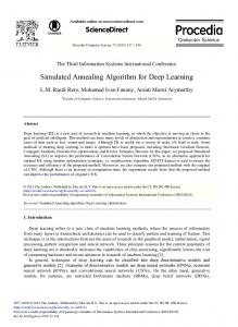
Figure 1: Mesh and contour plot of the objective function.

3. Simulated Experiment Results This section presents a simulation example (i.e., mixture normal model). The main purpose of this example is to demonstrate that the MTMSA algorithm could compute the optimization problem in the case of multiple local maxima and outperform its counterparts in terms of accuracy and efficiency. All results are obtained using R language (version X64 2.3.4) and MATLAB (version R2017a) on a Dell OptiPlex7020MT desktop computer with Intel(R) Core(TM) i74790 CPU @ 3.6 GHz, RAM 8.00 GB, and Windows 7 Ultimate with Service Pack 1 (x64). The R and MATLAB codes in this work are available upon request to the corresponding author. In this simulation example, we consider a two-dimensional multimodal mixture normal model modified from [27, 28]. In this model, the objective function is the probability density function, which is the combination of 20 normal models 20

2 󸀠 𝜔𝑖 exp−(1/2𝜎𝑖 )(x−𝜇i ) (x−𝜇i ) , 2 2𝜋𝜎 𝑖 𝑖=1

𝑓 (x) ∝ ∑

(5)

where 𝜎1 = 𝜎2 = ⋅ ⋅ ⋅ = 𝜎20 = 0.1 and (𝜔1 , 𝜔2 , . . . , 𝜔20 ), which are the weights of the 20 normal models, are chosen to be the arithmetic progression from 1 to 5, except the last one 𝜔20 = 10. The 20 mean vectors are independently sampled from the uniform distribution from [0, 10]. Figure 1 illustrates the mesh and contour plots of (5), which contains 20 modes in this objective function. This example poses a serious challenge for optimization because many classical optimization methods may converge on the local optimum in this multimodal example. Clearly, the global maximum point is the last mode (0.183, 7.501) with the maximum value of 2.449. Four methods are used to find the global maximum point of this optimization problem: the NM method, modified QN method, SA algorithm, and MTMSA algorithm. The NM and QN methods are commonly applied numerical optimization

algorithms, and the QN method allows box constraints. The SA and its improved version, i.e., the MTMSA algorithm, are stochastic optimization algorithms. Apart from the minimum temperature 𝑇𝑚𝑖𝑛 , another commonly used parameter that controls the degree of decreasing temperature is 𝑁𝑡𝑒𝑚𝑝𝑒𝑟 : 𝑇𝑘 = 𝑇𝑚𝑎𝑥 ⋅ 𝛼𝑘−1 , 𝑘 = 1, 2, . . . , 𝑁𝑡𝑒𝑚𝑝𝑒𝑟 .

(6)

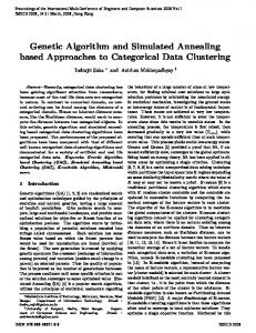
For the SA algorithm, we set the degree of decreasing temperature 𝑁𝑡𝑒𝑚𝑝𝑒𝑟 = 75, the starting temperature 𝑇𝑚𝑎𝑥 = 10, the decreasing parameter 𝛼 = 0.9, the length of the Markov chain 𝑁𝑚𝑐 = 100, and the proposal variance of the Metropolis algorithm V𝑝𝑟𝑜 = 2. For the MTMSA algorithm, we set the number of multiple-tries 𝑁𝑚𝑡𝑚 = 100. The other parameters are 𝑁𝑡𝑒𝑚𝑝𝑒𝑟 = 25, 𝛼 = 0.8, 𝑇𝑚𝑎𝑥 = 1, 𝑁𝑚𝑐 = 100, and V𝑝𝑟𝑜 = 2. With different 𝑁𝑡𝑒𝑚𝑝𝑒𝑟 (75 and 25) and 𝛼 (0.9 and 0.8, respectively) values, the SA and MTMSA algorithms have similar 𝑇𝑚𝑖𝑛 . We tested these four algorithms (NM, QN, SA, and MTMSA algorithms) to compute the optimization problem and repeated this computation 50 times. The computation results are summarized in Figure 2 and Table 1. The mean value, standard deviation (sd), mean square error (MSE), total CPU time (in seconds), and average CPU time for one accurate result (in seconds) of the results from different algorithms are summarized in Table 1, where 𝑚𝑒𝑎𝑛 = (1/𝑅) ∑𝑅𝑖=1 𝑉𝑖 , 𝑠𝑑 = √(1/(𝑅 − 1)) ∑𝑅𝑖=1 (𝑉𝑖 − 𝑚𝑒𝑎𝑛)2 ,

𝑀𝑆𝐸 = (1/𝑅) ∑𝑅𝑖=1 (𝑉𝑖 − 𝑉𝑒 )2 , and 𝑉𝑒 = 2.449 is the exact maximum value in the model (5). Figure 2 illustrates the boxplot of 50 computation results from these four algorithms. Suffering from the “local-trap” problem, NM and QN algorithms cannot find the global maximum successfully in 50 computations (they often find other local modes in (5)). Compared with the MTMSA algorithm, the SA algorithm uses a slowly decreasing temperature schedule (𝑁𝑡𝑒𝑚𝑝𝑒𝑟 = 75) and consumes more CPU time. However, only 10 results of 50 repetitions from the SA algorithm converge to the


5

Table 1: Computation results (mean, sd, MSE, consumed total CPU time, and average CPU time (in seconds)) of the 50 computations from different algorithms. DM 0.3447 0.4563 4.6319 4.1732 +∞

mean sd MSE total CPU time average CPU time

QN 0.0311 0.1355 5.8635 0.9121 +∞

2.5

SA 1.7523 0.6427 0.8901 1305.6 130.56

MTMSA 2.4392 0.0086 0.0001 528.1 10.562

Table 2: Biochemical oxygen demand versus time.

2

Time (days) 1 2 3 4 5 7

1.5 1 0.5 0 NM

QN

SA

BOD (mg/I) 8.3 10.3 19.0 16.0 15.6 19.8

MTMSA

Figure 2: Boxplot of 50 results computed from the NM method, QN method, SA algorithm, and MTMSA algorithm.

global maximum point (0.183, 7.501), and the mean of the SA algorithm is 1.7523. By contrast, the MTMSA algorithm functions with a rapidly decreasing temperature schedule. The MTMSA algorithm consumes minimal CPU time (only about 8 min), but it yields highly accurate results (all 50 results converge to the global maximum). Furthermore, the MTMSA algorithm only needs approximately 10 seconds to compute one accurate result, whereas the SA algorithm requires about 130 seconds. All results from NM and QN algorithms suffer from the “local-trap” problem. We compared the differences in the decreasing temperature schedules used in SA and MTMSA algorithms. “The slower the better” was found to be applicable to the decreasing temperature schedules. A rapidly decreasing temperature schedule may result in the “local-trap” problem. In the next simulation, we set the temperature schedules to decrease from 10 to 5 × 10−3 , and the length of decreasing temperature was set to 500, 75 and 25 for SA and MTMSA algorithms. Each computation was repeated 50 times. The length of decreasing temperature of the SA algorithm is set to 75, 500, and denoted as the SA1 and SA2 algorithm, respectively. The SA2 algorithm shows the slowest decreasing schedule. It uses 500 steps to drop from the highest temperature to the lowest one. Thus almost all 50 results converge to the global maximum (about 94% percent of computation results escape from local optima and reaches the global maximum). The SA1 algorithm uses a rapidly decreasing schedule, and only about half of the 50 results converge to the global maximum (about 54% percent of computation results escape from local optima and reaches the global maximum). By contrast, the MTMSA algorithm only uses 25 steps in decreasing temperature, but all of the 50 results converge to the global maximum.

Figure 3 shows the decreasing schedules and convergence paths of the three algorithms. We find that when the temperature decreases to about 0.02 (corresponding to the 50th, 400th, and 20th steps in SA1, SA2, and MTMSA), all sample paths from the three algorithms converge to their local and global optima. All the sample paths of MTMSA converge to the global optima, and lots of sample paths of SA1 and SA2 converge to the local optima because the average sample path of MTMSA in Figure 3 is the highest and at the level about 2.43. The MTMSA algorithm uses the rapidly decreasing schedule and achieves the fastest convergence rate. Therefore, the MTMSA algorithm is the most efficient and accurate in this simulation example.

4. Real Data Examples 4.1. Bayesian Analysis Using MTMSA. In this section, we illustrate the application of the MTMSA algorithm in Bayesian analysis with real data from [29]. In this example, we fit a nonlinear model derived from exponential decay 𝑦𝑖 = 𝜃1 (1 − exp {−𝜃2 𝑥𝑖 }) + 𝜀𝑖 ,

𝜀𝑖 ∼ 𝑁 (0, 𝜎2 ) ,

(7)

with a fixed rate that is constant to a real data set [30] (Table 2). The variables BOD (mg/I)) and time (days) in Table 2 are the response and control variables in model (7) (denoted as the BOD problem) with a constant variance 𝜎2 for independent normal errors. The likelihood for the BOD problem is 𝐿 (𝜃1 , 𝜃2 , 𝜎2 | 𝑋, 𝑌) ∝ exp {−6 log 𝜎 6

2

1 ∑𝑖=1 (𝑦𝑖 − 𝜃1 (1 − exp {−𝜃2 𝑥𝑖 })) }, − 2 𝜎2 where 𝑋 = (𝑥1 , . . . , 𝑥6 ) and 𝑌 = (𝑦1 , . . . , 𝑦6 ).

(8)

6

Mathematical Problems in Engineering 2.5

10 9

2

8 Markov chain path

Temperature

7 6 5 4 3

1.5

1

0.5

2 1 0

0

50

100 150 200 250 300 350 400 450 500 Step

the SA1 algorithm the SA2 algorithm the MTMSA algorithm

0

0

50

100 150 200 250 300 350 400 450 500 Temperature step

the SA1 algorithm the SA2 algorithm the MTMSA algorithm

(a) The decreasing temperature schedules

(b) The convergence paths of different algorithms

Figure 3: Decreasing temperature schedules (a) and convergence paths (b) of the SA1 algorithm, SA2 algorithm, and MTMSA algorithm. The convergence paths are the average of 50 paths. Table 3: Computation results (mean (10−5 ), sd (10−5 )) in special temperature steps (1, 5, 10, 15, 20, 25) from 20 repetitions. step 1 1.05 3.57

mean sd

step 5 1.39 5.16

step 10 0.91 2.20

While choosing the flat prior for the parameters 𝜎2 and (𝜃1 , 𝜃2 ) (i.e., the uniform distribution in (0, +∞) and [−20, 50] × [−2, 6], respectively) and integrating out 𝜎2 , we obtain the following (improper) posterior distribution of (𝜃1 , 𝜃2 ): 𝑝 (𝜃1 , 𝜃2 | 𝑋, 𝑌) 6

2

−2

∝ [∑ (𝑦𝑖 − 𝜃1 (1 − exp {−𝜃2 𝑥𝑖 })) ]

(9)

𝑖=1

⋅ 𝐼[−20,50]×[−2,6] (𝜃1 , 𝜃2 ) , where 𝐼[−20,50]×[−2,6] (𝜃1 , 𝜃2 ) {1, ={ 0, {

(𝜃1 , 𝜃2 ) ∈ [−20, 50] × [−2, 6]

(10)

(𝜃1 , 𝜃2 ) ∉ [−20, 50] × [−2, 6] .

For a Bayesian analysis, one often treats the parameters (𝜃1 , 𝜃2 ) as random variables. In this work, we use the posterior distribution of (𝜃1 , 𝜃2 ) for their statistical inference and use the posterior mode of (9) as the estimation of (𝜃1 , 𝜃2 ), which coincides with the maximum likelihood estimation. The Bayesian statistical inference of the parameters (𝜃1 , 𝜃2 ) is

step 15 3.92 12.2

step 20 145 3.04

step 25 148 0.24

translated to the global optimization problem in [−20, 50] × [−2, 6]. sup

𝑝 (𝜃1 , 𝜃2 | 𝑋, 𝑌) .

(𝜃1 ,𝜃2 )∈[−20,50]×[−2,6]

(11)

In addition, we use the MTMSA algorithm to compute the global optimization problem (11). The parameters of the MTMSA algorithm are set to be 𝑁𝑚𝑡𝑚 = 20, 𝑁𝑡𝑒𝑚𝑝𝑒𝑟 = 25, 𝛼 = 0.6, 𝑇𝑚𝑎𝑥 = 1, and 𝑁𝑚𝑐 = 1000. The computation is then repeated 20 times. Figure 4 and Table 3 illustrate the decreasing temperature schedule and the convergence paths of 20 repetitions from the MTMSA algorithm. After 20 steps, all 20 computation paths become convergent to 1.48 × 10−3 , which has the largest mean and smallest sd. Figure 5 shows the mesh (a) and contour (b) plots of the posterior distribution (9). Figure 6 and Table 4 show the locations of the scatters (𝜃1 , 𝜃2 ) from 20 repetitions at different temperature steps. With the temperature decreasing from 0.6 to 2.8×10−6 , all scatters converge to the optimization point (19.15, 0.53). 4.2. Half-Space Depth Computation Using MTMSA. As a powerful tool for nonparametric multivariate analysis, halfspace depth (HD also known as Tukey depth) has been eliciting increased interest since it was introduced by Tukey [31, 32]. HD, which extends univariate order-related statistics to multivariate settings, provides a center-outward ordering


7

Table 4: Location results of (𝜃1 , 𝜃2 ) at different temperature levels. Level mean sd

2.8 × 10−4 (16.63, 1.06) (17.64, 1.92)

0.6 (20.22, 1.80) (21.71, 2.39)

1.6 × 10−4 (18.25, 1.05) (9.58, 1.56)

1.5

0.6

2.8 × 10−6 (19.15, 0.53) (0.11, 0.01)

×10-3

0.5 1 Value

Temperature

0.4 0.3

0.5

0.2 0.1 0

0

5

10

15

20

0

25

0

5

10

Step

15

20

25

Step

(a)

(b)

Figure 4: The decreasing temperature schedule (a) and the convergence paths of 20 repetitions (b) from the MTMSA algorithm. 6 5

×10 -4

4 3

5

2

p

2

10

1

0

0

−5 6

−1

4 2 2

0 −2

−20

20

0

40 −2 −20

−10

0

10

20

30

40

50

1

1

(a) Mesh plot of posterior distribution

(b) Contour plot of posterior distribution

Figure 5: Exact mesh (a) and contour (b) plots of the posterior distribution (9).

of multivariate samples and visualizes data in high dimensional cases [33, 34]. However, the computation of HD is challenging, and the exact algorithm is often inefficient, especially when the dimension is high [35]. In this subsection, we use MTMSA to compute HD and compared MTMSA with other approximated and exact algorithms.

Given a sample data set of size 𝑛 X𝑛 = {X1 , X2 , . . . , X𝑛 } in R , x is a point in R𝑑 , and the HD of x with respect to (w.r.t.) X𝑛 is defined by 𝑑

1 𝐻𝐷 (x, X𝑛 ) = min # {𝑖 | u𝑇 X𝑖 ≥ u𝑇 x, 𝑖 ∈ N} , u∈S𝑑−1 𝑛

(12)

Mathematical Problems in Engineering 6

6

5

5

4

4

3

3

2

2

2

2

8

1

1

0

0

−1

−1

−2 −20

−10

0

10

20

30

40

−2 −20

50

−10

0

10

6

5

5

4

4

3

3

2

2

1

1

0

0

−1

−1

−10

0

30

40

50

20

30

40

50

(b)

2

2

(a)

6

−2 −20

20 1

1

10

20

30

40

50

−2 −20

−10

0

10 1

1 (c)

(d)

Figure 6: Locations of (𝜃1 , 𝜃2 ) from 20 repetitions at different temperature steps (0.6, 2.8 × 10−4 , 1.6 × 10−4 , 2.8 × 10−6 , ).

where S𝑑−1 = {𝑢 ∈ R𝑑 | ‖𝑢‖ = 1}, N = {1, 2, . . . , 𝑛}, and #{⋅} denotes the counting measure. Then, the computation of HD (12) is a global optimization problem in S𝑑−1 . Next, we considered a concrete data set (Table 6) obtained from [35] and can be found in the Records Office of the Laboratory School of the University of Chicago. The original data consisted of 64 subjects’ scores obtained from eighthgrade levels to eleventh-grade levels. Then, we compared MTMSA with three approximated algorithms (NM, QN, and SA) and the exact algorithm from [35] for the HD computation of the first data point w.r.t. the data set.

We tested two sets of parameters for the SA algorithm. The first is 𝑁𝑡𝑒𝑚𝑝𝑒𝑟 = 20, 𝑁𝑚𝑐 = 50, 𝑇𝑚𝑎𝑥 = 1, and 𝑎 = 0.7 and denoted as the SA1 algorithm. The second one is 𝑁𝑡𝑒𝑚𝑝𝑒r = 20, 𝑁𝑚𝑐 = 200, 𝑇𝑚𝑎𝑥 = 1, and 𝑎 = 0.7 and denoted as the SA2 algorithm. For the MTMSA algorithm, we set the parameter to be 𝑁𝑡𝑒𝑚𝑝𝑒𝑟 = 20, 𝑚 = 100, 𝑁𝑚𝑐 = 30, 𝑇𝑚𝑎𝑥 = 1, and 𝑎 = 0.7. The three algorithms (SA1, SA2, and MTMSA) use the same decreasing temperature schedule. Then, we used the six algorithms (exact, NM, QN, SA1, SA2, and MTMSA) for this computation and repeated the computation 50 times. Figure 7 and Table 5 show the computation results.


9

Table 5: Computation results (mean, sd, MSE, consumed total CPU time, and average CPU time (in seconds)) of the 50 computations from different algorithms. exact 0.2344 0 0 2450 49

mean sd MSE total CPU time average CPU time

NM 0.3653 0.0519 0.0199 0.06 +∞

QN 0.3841 0.0485 0.0247 0.05 +∞

SA1 0.2609 0.0243 0.0013 5.7410 0.9570

Table 6: Concrete data set. subject 1 2 3 4 5 6 7 8 9 10 11 12 13 14 15 16 17 18 19 20 21 22 23 24 25 26 27 28 29 30 31 32 33 34 35 36 37 38 39

SA2 0.2425 0.0079 0.0001 23.103 0.9626

MTMSA 0.2344 0 0 15.87 0.3174

Table 6: Continued.

Grade 8

Grade 9

Grade 10

Grade 11

1.75 0.90 0.80 2.42 −1.31 −1.56 1.09 −1.92 −1.61 2.47 −0.95 1.66 2.07 3.30 2.75 2.25 2.08 0.14 0.13 2.19 −0.64 2.02 2.05 1.48 1.97 1.35 −0.56 0.26 1.22 −1.43 −1.17 1.68 −0.47 2.18 4.21 8.26 1.24 5.94 0.87

2.60 2.47 0.93 4.15 −1.31 1.67 1.50 1.03 0.29 3.64 0.41 2.74 4.92 6.10 2.53 3.38 1.74 0.01 3.19 2.65 −1.31 3.45 1.80 0.47 2.54 4.63 −0.36 0.08 1.41 0.80 1.66 1.71 0.93 6.42 7.08 9.55 4.90 6.56 3.36

3.76 2.44 0.40 4.56 −0.66 0.18 0.52 0.50 0.73 2.87 0.21 2.40 4.46 7.19 4.28 5.79 4.12 1.48 0.60 3.27 −0.37 5.32 3.91 3.63 3.26 3.54 1.14 1.17 4.66 −0.03 2.11 4.07 1.30 4.64 6.00 10.24 2.42 9.36 2.58

3.68 3.43 2.27 4.21 −2.22 2.33 2.33 3.04 3.24 5.38 1.82 2.17 4.71 7.46 5.93 4.40 3.62 2.78 3.14 2.73 4.09 6.01 2.49 3.88 5.62 5.24 1.34 2.15 2.62 1.04 1.42 3.30 0.76 4.82 5.65 10.58 2.54 7.72 1.73

subject 40 41 42 43 44 45 46 47 48 49 50 51 52 53 54 55 56 57 58 59 60 61 62 63 64

Grade 8 −0.09 3.24 1.03 3.58 1.41 −0.65 1.52 0.57 2.18 1.10 0.15 −1.27 2.81 2.62 0.11 0.61 −2.19 1.55 0.04 3.10 −0.29 2.28 2.57 −2.19 −0.04

Grade 9 2.29 4.78 2.10 4.67 1.75 −0.11 3.04 2.71 2.96 2.65 2.69 1.26 5.19 3.54 2.25 1.14 −0.42 2.42 0.50 2.00 2.62 3.39 5.78 0.71 2.44

Grade 10 3.08 3.52 3.88 3.83 3.70 2.40 2.74 1.90 4.78 1.72 2.69 0.71 6.33 4.86 1.56 1.35 1.54 1.11 2.60 3.92 1.60 4.91 5.12 1.56 1.79

Grade 11 3.35 4.84 2.81 5.19 3.77 3.53 2.63 2.41 3.34 2.96 3.50 2.68 5.93 5.80 3.92 0.53 1.16 2.18 2.61 3.91 1.86 3.89 4.98 2.31 2.64

Figure 7 and Table 5 show that the exact algorithm consumed the most CPU time (about 2450 seconds) and obtained exact computation results (0.2344). MTMSA also obtained the exact results but consumed only 15.87 seconds. The SA algorithms (SA1 and SA2) consumed suitable CPU time (5.741 and 23.103 seconds, respectively) but obtained only 6 and 24 exact results, respectively. The results of NM and QN fell into the local optima because all of them were larger than the exact result. With regard to the average CPU time, MTMSA used only 0.3174 for the computation of one exact result, which is the least amount of time compared with the time for the other exact and approximated algorithms. Hence, MTMSA outperformed the other algorithms in this experiment example.

10


Acknowledgments

0.5

The research was partially supported by the National Natural Science Foundation of China (11501320, 71471101, and 11426143), the Natural Science Foundation of Shandong Province (ZR2014AP008), and the Natural Science Foundation of Qufu Normal University (bsqd20130114).

0.45 0.4 0.35

References

0.3 0.25 Exact

NM

QN

SA1

SA2

MTMSA

Figure 7: Boxplot of the results computed from the exact, NM, QN, SA1, SA2, and MTMSA algorithms.

5. Conclusions We developed the MTMSA algorithm for global optimization problems in the fields of mathematical/biological sciences, engineering, Bayesian data analysis, operational research, life sciences, and so on. The MTMSA algorithm is a combination of the SA algorithm and the MTM algorithm. Using simulated and real data examples, it demonstrated that, relative to the QN and SA algorithm, the MTMSA algorithm can function with a rapidly decreasing cooling schedule while guaranteeing that the global energy minima are reached. Several directions can be taken for future work. First, combined with the quasi-Monte Carlo method, the lowdiscrepancy sequences and experimental design [36–39] can be used to accelerate the convergence of the SA algorithm. Second, aside from the MTM algorithm, the MTMSA algorithm can also be implemented with several parallel interacting Markov chains to improve the SA algorithm by making full use of modern multicore computer [40, 41]. Third, we anticipate that a parallel SA algorithm can be used efficiently for variable selection in high dimensional cases [42–45] because the variable selection problem is a special case of the optimization problem. Finally, data depth [32, 33, 35, 46] is an important tool for multidimensional data analysis, but the computation of data depth in high dimensional cases is challenging. The example of half-space depth computation in Section 4 shows the advantage of the MTMSA algorithm in low dimensional case. Hence, we believe that the MTMSA algorithm can be successfully applied to compute highly complex data depths (e.g., projection and regression depths) in high dimensional cases. Further analysis along these directions would be interesting.

Data Availability The data used to support the findings of this study are available from the corresponding author upon request.

Conflicts of Interest The authors declare that they have no conflicts of interest regarding the publication of this paper.

[1] J. S. Liu, Monte Carlo Strategies in Scientific Computing, Springer, 2001. [2] F. Liang, C. Liu, and R. J. Carroll, Advanced Markov Chain Monte Carlo Methods: Learning From Past Samples, John Wiley & Sons, 2011. [3] S. Kirkpatrick, J. Gelatt, and M. P. Vecchi, “Optimization by simulated annealing,” American Association for the Advancement of Science: Science, vol. 220, no. 4598, pp. 671–680, 1983. [4] Y. Wang, L. Qi, S. Luo, and Y. Xu, “An alternative steepest direction method for the optimization in evaluating geometric discord,” Pacific Journal of Optimization, vol. 10, no. 1, pp. 137– 149, 2014. [5] C. Wang and Y. Wang, “A superlinearly convergent projection method for constrained systems of nonlinear equations,” Journal of Global Optimization, vol. 44, no. 2, pp. 283–296, 2009. [6] Y. Wang, L. Caccetta, and G. Zhou, “Convergence analysis of a block improvement method for polynomial optimization over unit spheres,” Numerical Linear Algebra with Applications, vol. 22, no. 6, pp. 1059–1076, 2015. [7] L. Qi, X. Tong, and Y. Wang, “Computing power system parameters to maximize the small signal stability margin based on min-max models,” Optimization and Engineering, vol. 10, no. 4, pp. 465–476, 2009. [8] H. Chen, Y. Chen, G. Li, and L. Qi, “A semidefinite program approach for computing the maximum eigenvalue of a class of structured tensors and its applications in hypergraphs and copositivity test,” Numerical Linear Algebra with Applications, vol. 25, no. 1, 2018. [9] G. Wang and X. X. Huang, “Levitin-Polyak well-posedness for optimization problems with generalized equilibrium constraints,” Journal of Optimization Theory and Applications, vol. 153, no. 1, pp. 27–41, 2012. [10] G. Wang, “Levitin-Polyak well-posedness for vector optimization problems with generalized equilibrium constraints,” Pacific Journal of Optimization, vol. 8, no. 3, pp. 565–576, 2012. [11] S. Geman and D. Geman, “Stochastic relaxation, gibbs distributions, and the Bayesian restoration of images,” IEEE Transactions on Pattern Analysis and Machine Intelligence, vol. 6, no. 6, pp. 721–741, 1984. [12] R. A. Holley, S. Kusuoka, and D. W. Stroock, “Asymptotics of the spectral gap with applications to the theory of simulated annealing,” Journal of Functional Analysis, vol. 83, no. 2, pp. 333– 347, 1989. [13] F. Liang, C. Liu, and R. J. Carroll, “Stochastic approximation in Monte Carlo computation,” Journal of the American Statistical Association, vol. 102, no. 477, pp. 305–320, 2007. [14] F. Liang, Y. Cheng, and G. Lin, “Simulated stochastic approximation annealing for global optimization with a square-root cooling schedule,” Journal of the American Statistical Association, vol. 109, no. 506, pp. 847–863, 2014.

Mathematical Problems in Engineering [15] G. Karagiannis, B. A. Konomi, G. Lin, and F. Liang, “Parallel and interacting stochastic approximation annealing algorithms for global optimisation,” Statistics and Computing, vol. 27, no. 4, pp. 927–945, 2017. [16] J. S. Liu, F. Liang, and W. H. Wong, “The multiple-try method and local optimization in metropolis sampling,” Journal of the American Statistical Association, vol. 95, no. 449, pp. 121–134, 2000. [17] R. Casarin, R. Craiu, and F. Leisen, “Interacting multiple try algorithms with different proposal distributions,” Statistics and Computing, vol. 23, no. 2, pp. 185–200, 2013. [18] N. Metropolis, A. W. Rosenbluth, M. N. Rosenbluth, A. H. Teller, and E. Teller, “Equation of state calculations by fast computing machines,” The Journal of Chemical Physics, vol. 21, no. 6, pp. 1087–1092, 1953. [19] W. Shao, G. Guo, F. Meng, and S. Jia, “An efficient proposal distribution for metropolis-hastings using a b-splines technique,” Computational Statistics & Data Analysis, vol. 57, pp. 465–478, 2013. [20] W. Shao and Y. Zuo, “Simulated annealing for higher dimensional projection depth,” Computational Statistics & Data Analysis, vol. 56, no. 12, pp. 4026–4036, 2012. [21] W. Shao, G. Guo, G. Zhao, and F. Meng, “Simulated annealing for the bounds of kendall’s tau and spearman’s rho,” Journal of Statistical Computation and Simulation, vol. 84, no. 12, pp. 2688– 2699, 2014. [22] Y. Luo, B. Zhu, and Y. Tang, “Simulated annealing algorithm for optimal capital growth,” Physica A: Statistical Mechanics and its Applications, vol. 408, pp. 10–18, 2014. [23] O. S. Sarıyer and C. G¨uven, “Simulated annealing algorithm for optimal capital growth,” Physica A: Statistical Mechanics and its Applications, vol. 408, pp. 10–18, 2014. [24] W. K. Hastings, “Monte Carlo sampling methods using Markov chains and their applications,” Biometrika, vol. 57, no. 1, pp. 97– 109, 1970. [25] J. A. Nelder and R. Mead, “A simplex method for function minimization,” The Computer Journal, vol. 7, no. 4, pp. 308–313, 1965. [26] R. H. Byrd, P. Lu, J. Nocedal, and C. Y. Zhu, “A limited memory algorithm for bound constrained optimization,” SIAM Journal on Scientific Computing, vol. 16, no. 5, pp. 1190–1208, 1995. [27] S. C. Kou, Q. Zhou, and W. H. Wong, “Equi-energy sampler with applications in statistical inference and statistical mechanics,” The Annals of Statistics, vol. 34, no. 4, pp. 1581–1652, 2006. [28] F. Liang and W. H. Wong, “Real-parameter evolutionary Monte Carlo with applications to Bayesian mixture models,” Journal of the American Statistical Association, vol. 96, no. 454, pp. 653– 666, 2001. [29] C. Ritter and M. A. Tanner, “Facilitating the Gibbs sampler: The Gibbs stopper and the Griddy–Gibbs sampler,” Journal of the American Statistical Association, vol. 87, no. 419, pp. 861–868, 1992. [30] D. M. Bates and D. G. Watts, Nonlinear Regression Analysis and Its Applications, John Wiley & Sons, New York, NY, USA, 1988. [31] J. W. Tukey, “Mathematics and the picturing of data,” Proceedings of the International Congress of Mathematicians, vol. 2, pp. 523–531, 1975. [32] Y. Zuo and R. Serfling, “General notions of statistical depth function,” The Annals of Statistics, vol. 28, no. 2, pp. 461–482, 2000. [33] X. Liu, Y. Zuo, and Q. Wang, “Finite sample breakdown point of Tukey’s halfspace median,” Science China Mathematics, vol. 60, no. 5, pp. 861–874, 2017.

11 [34] X. Liu, “Fast implementation of the Tukey depth,” Computational Statistics, vol. 32, no. 4, pp. 1395–1410, 2017. [35] X. Liu and Y. Zuo, “Computing halfspace depth and regression depth,” Communications in Statistics—Simulation and Computation, vol. 43, no. 5, pp. 969–985, 2014. [36] Z. Li, S. Zhao, and R. Zhang, “On general minimum lower order confounding criterion for s-level regular designs,” Statistics & Probability Letters, vol. 99, pp. 202–209, 2015. [37] J. Wang, Y. Yuan, and S. Zhao, “Fractional factorial splitplot designs with two- and four-level factors containing clear effects,” Communications in Statistics—Theory and Methods, vol. 44, no. 4, pp. 671–682, 2015. [38] S. Zhao, D. K. Lin, and P. Li, “A note on the construction of blocked two-level designs with general minimum lower order confounding,” Journal of Statistical Planning and Inference, vol. 172, pp. 16–22, 2016. [39] S.-L. Zhao and Q. Sun, “On constructing general minimum lower order confounding two-level block designs,” Communications in Statistics—Theory and Methods, vol. 46, no. 3, pp. 1261– 1274, 2017. [40] G. Guo, W. You, G. Qian, and W. Shao, “Parallel maximum likelihood estimator for multiple linear regression models,” Journal of Computational and Applied Mathematics, vol. 273, pp. 251–263, 2015. [41] G. Guo, W. Shao, L. Lin, and X. Zhu, “Parallel tempering for dynamic generalized linear models,” Communications in Statistics—Theory and Methods, vol. 45, no. 21, pp. 6299–6310, 2016. [42] M. Wang and G.-L. Tian, “Robust group non-convex estimations for high-dimensional partially linear models,” Journal of Nonparametric Statistics, vol. 28, no. 1, pp. 49–67, 2016. [43] M. Wang, L. Song, and G.-l. Tian, “Scad-penalized least absolute deviation regression in high-dimensional models,” Communications in Statistics—Theory and Methods, vol. 44, no. 12, pp. 2452–2472, 2015. [44] G.-L. Tian, M. Wang, and L. Song, “Variable selection in the high-dimensional continuous generalized linear model with current status data,” Journal of Applied Statistics, vol. 41, no. 3, pp. 467–483, 2014. [45] M. Wang and X. Wang, “Adaptive Lasso estimators for ultrahigh dimensional generalized linear models,” Statistics & Probability Letters, vol. 89, pp. 41–50, 2014. [46] P. J. Rousseeuw and M. Hubert, “Regression depth,” Journal of the American Statistical Association, vol. 94, no. 446, pp. 388– 433, 1999.

Advances in

Operations Research Hindawi www.hindawi.com

Volume 2018

Advances in

Decision Sciences Hindawi www.hindawi.com

Volume 2018

Journal of

Applied Mathematics Hindawi www.hindawi.com

Volume 2018

The Scientific World Journal Hindawi Publishing Corporation http://www.hindawi.com www.hindawi.com

Volume 2018 2013

Journal of

Probability and Statistics Hindawi www.hindawi.com

Volume 2018

International Journal of Mathematics and Mathematical Sciences

Journal of

Optimization Hindawi www.hindawi.com

Hindawi www.hindawi.com

Volume 2018

Volume 2018

Submit your manuscripts at www.hindawi.com International Journal of

Engineering Mathematics Hindawi www.hindawi.com

International Journal of

Analysis

Journal of

Complex Analysis Hindawi www.hindawi.com

Volume 2018


Stochastic Analysis Hindawi www.hindawi.com


Volume 2018

Volume 2018

Advances in

Numerical Analysis Hindawi www.hindawi.com

Volume 2018

Journal of


Volume 2018

Journal of

Mathematics Hindawi www.hindawi.com


Function Spaces Volume 2018


Volume 2018


Differential Equations Hindawi www.hindawi.com

Volume 2018

Abstract and Applied Analysis Hindawi www.hindawi.com

Volume 2018

Discrete Dynamics in Nature and Society Hindawi www.hindawi.com

Volume 2018

Advances in

Mathematical Physics Volume 2018


Volume 2018