technology have been developed to classify ice-free ocean surfaces. Neural networks ... Sensing Research Group, Florida Institute of Technology, Melbourne, FL. 32901 USA. ...... in the Florida. Tech Remote Sensing Research Group, FIT. His.
IEEE TRANSACTIONS ON GEOSCIENCE AND REMOTE SENSING, VOL. 35, NO. 4, JULY 1997
817
A Neural Network Algorithm for Sea Ice Edge Classification Sami M. Alhumaidi, W. Linwood Jones, Senior Member, IEEE, Jun-Dong Park, and Shannon M. Ferguson
Abstract— The NASA Scatterometer (NSCAT), launched in August 1996, is designed to measure wind vectors over ice-free oceans. To prevent contamination of the wind measurements, by the presence of sea ice, algorithms based on neural network technology have been developed to classify ice-free ocean surfaces. Neural networks trained using polarized alone and polarized plus multi-azimuth “look” Ku-band backscatter are described. Algorithm skill in locating the sea ice edge around Antarctica is experimentally evaluated using backscatter data from the Seasat-A Satellite Scatterometer that operated in 1978. Comparisons between the algorithms demonstrate a slight advantage of combined polarization and multi-look over using co-polarized backscatter alone. Classification skill is evaluated by comparisons with surface truth (sea ice maps), subjective ice classification, and independent over lapping scatterometer measurements (consecutive revolutions).
I. INTRODUCTION N AUGUST 1996, the NASA Scatterometer (NSCAT) was launched on Japan’s Advanced Earth Observation Satellite (ADEOS) to measure the surface winds over the world’s ice-free oceans. Since land or ice within the antenna instantaneous field of view (IFOV) will contaminate the ocean wind measurement, it is necessary to identify and remove measurements so affected. For land, the process is relatively simple; however, for sea ice, it is more difficult because the extent of the ice is unknown a priori. This paper describes a convenient and timely technique for determining the sea ice boundary from the NSCAT backscatter data alone.
I
A. Applicability of Neural Nets Neural nets have been successfully used for classifying radar backscatter from sea ice [1]–[3]. Although neural nets vary greatly depending on their architectures, learning rules, activation functions, etc., they can be classified into two main categories, supervised nets and unsupervised nets. In a supervised neural network implementation, the classes associated with the training data are available and are used by the net to improve performance. Once the net has learned the training data, a comparable set of data, known as the testing data set, is presented to the net without any class information. This set is classified by the net, and the classification results are Manuscript received September 9, 1996; revised March 3, 1997. This work was supported under contract to the Jet Propulsion Laboratory–NASA Scatterometer Project. S. M. Alhumaidi and S. M. Ferguson are with the Florida Technical Remote Sensing Research Group, Florida Institute of Technology, Melbourne, FL 32901 USA. W. L. Jones and J.-D. Park are with the Central Florida Remote Sensing Laboratory, Electrical and Computer Engineering Department, University of Central Florida, Orlando, FL 32816 USA. Publisher Item Identifier S 0196-2892(97)04472-0.
compared with the known classes of the testing data. In fact, once the training phase of a neural net is completed, both data sets, training and testing, must be classified by the net and the result determines how well the net was able to learn the classes. For example, if the error produced by classifying the training data was very small while the error classifying the testing data was large, then one concludes that the net “memorized” the training data well but has poor generalization skill. Depending on the type of neural network implementation applied, the effects of this problem can be decreased by presenting the training data less frequently during training and/or modifying some learning parameters [4]. In general, a higher classification accuracy can be reached using supervised neural nets than with unsupervised techniques. However, an independent reliable classifier must be used to classify the training and testing data before a supervised neural net can be implemented. Any errors associated with this independent classification can be transferred to the neural net results causing further errors. For this study, care was taken to insure that the training set contained only ice-free ocean or 100% first-year sea ice. On the other hand, training data for an unsupervised net need not be classified by an independent classifier. For this case, the net processes the input data by finding natural clustering occurring in the data and assigning a different class number to each cluster. Depending on the degree of overlap among the classes in the input-data space, one would expect significant differences between these two approaches. The performance of unsupervised nets can degrade quickly with increasing percentage overlap of the input data; whereas, the performance of supervised neural nets would degrade more slowly [4]. B. Present Application In this work, we applied both types of neural nets to develop algorithms to infer the extent of first-year sea ice using Ku-band radar backscatter measurements. Because NSCAT measurements were not yet available, we used Seasat-A Satellite Scatterometer (SASS) [5] data. SASS operated onboard the Seasat-A satellite during the Summer-Fall 1978; and during this period, valuable sea ice measurements were obtained in both the Arctic and Antarctic regions. Because the Arctic observations occurred during the summer melt season, the backscatter response was complicated and not used in this work. Future investigations using NSCAT will evaluate these sea ice classification algorithms in the Arctic and Antarctic over a full-year period. Thus, we have trained and tested the neural networks during the Antarctic winter where only first year sea ice is present.
0196–2892/97$10.00 1997 IEEE
818
IEEE TRANSACTIONS ON GEOSCIENCE AND REMOTE SENSING, VOL. 35, NO. 4, JULY 1997
Fig. 2. NSCAT sigma-0 cell sampling.
Fig. 1. NSCAT measurement Geometry.
Even though the multilayer perceptron (MLP) neural net is the usual choice in solving similar types of problems, three types of neural nets were evaluated in this study. The two supervised neural nets tested were the multilayer perceptron net, and the more biologically plausible, supervised fuzzy adaptive resonance theory net (FARTMAP). Further, an unsupervised net based on the fuzzy ART algorithm was tested for completeness. The three nets were trained and then tested using the same input radar measurement parameters and SASS data sets. Also, a reduced data set was generated by eliminating an input parameter. A second MLP net was trained on the reduced data set, and the classification results of the various nets were compared. II. SATELLITE SCATTEROMETERS A. The NASA Scatterometer, NSCAT A brief overview of the NSCAT instrument [6] and its measurement geometry is presented. The NSCAT is a radar system that measures the ocean backscatter to determine the surface scattering coefficient or normalized radar cross section, sigma0. The NSCAT measurements are obtained within two swaths as illustrated in Fig. 1. Each swath is illuminated by four “fan beam” antennas (beams) at three azimuths. The middle azimuth has two antennas to measure dual polarized (vertical and horizontal) sigma-0’s at this position. The instrument uses Doppler processing to subdivide each antenna footprint into twenty four sigma-0 measurements. In each swath, these measurements from the four antennas are first collocated into 25 km “sigma-0 cells” (Fig. 2). Collocation accuracy for the four antenna beam sigma-0’s is typically better than 10 km. Next, four sigma-0 cells are grouped together to form 50-km wind vector cells, WVC. At the WVC, the resulting 16 sigma0’s are processed to infer a single surface wind vector. For purposes of NSCAT wind retrievals, the individual sigma-0
cells must be flagged as ocean, land or ice before wind vector processing can occur. Because our algorithm uses multiple sigma-0’s to achieve classification, we will produce an “ice flag” (ice edge location) at 25-km resolution. For accurate wind measurements, it is important that all sigma-0’s are for only ocean i.e., no land or sea ice within the individual sigma-0 measurement instantaneous field of view (IFOV). Thus, it is necessary to identify and remove sigma-0 measurements so affected. For land, the process is relatively simple using land maps and knowledge of the earth geolocated antenna IFOV’s. For sea ice, it is more difficult to identify its time dependent extent. Because of its dynamic nature, the sea ice boundary is usually determined from a variety of satellite remote sensing data e.g., visible, infrared and passive microwave. However, the nonsimultaneity of these measurements with ADEOS can lead to significant errors (collocation and temporal changes in ice edge) as well as increased complexity in the NSCAT data processing. This paper presents three candidate neural network algorithms that are capable of detecting the presence of first year sea ice within the sub-WVC (25-km resolution) using NSCAT sigma-0’s alone. These algorithms can be easily implemented to provide efficient sea ice classification “on the fly” and thereby ensure “stand alone” capability for the NSCAT data processing. B. The Seasat-A Satellite Scatterometer—SASS A detailed description of the SASS instrument and sigma0 measurement is given in [5] and [7]. The SASS geometry was very similar to NSCAT except that over each swath it obtained sigma-0’s from two beams (instead of three azimuth directions—middle antenna deleted), and for SASS, all beams were dual polarized. Thus, the measurement geometry had antenna beams located 90 apart in azimuth. SASS used Doppler filters to subdivide the antenna beams into twelve sigma-0 measurements (instead of 24 for NSCAT) with IFOV dimensions of about 15 70 km sampled on 50 km centers along and across the satellite track. The forward and aft beams were sampled in time to produce collocated surface
ALHUMAIDI et al.: NEURAL NETWORK ALGORITHM FOR SEA ICE EDGE CLASSIFICATION
measurements on a 50 km grid. SASS hardware limitations caused relatively poor collocation for multiple azimuth sigma0’s ( 25 km). Because of the similar measurement geometrys, SASS produces an excellent simulation scenario except that NSCAT has improved spatial resolution by a factor of two i.e., 25 km versus 50 km. For NSCAT use, the neural net algorithms will use dual polarized data from NSCAT beams 2 and 3 (and beams 6 and 7). These were simulated using dual polarized sigma-0’s from forward and aft looking SASS beams. Also, some neural net algorithms will use multi-azimuth look data from NSCAT beams 1 and 4 (left hand swath—beams 5 and 8). These data were simulated using vertical sigma-0’s from forward and aft looking SASS beams. Sigma-0’s from different beams were collocated by selecting the “closest neighbors” at a given surface location. For the dual polarized data, collocation was trivial because SASS dual polarized data resulted from IFOV’s that overlapped by about 50%. For multi-azimuth look data, collocation was considerably more difficult. For this case, we paired sigma-0’s for the required beams whenever the centers of the IFOV’s were within 25 km. This resulted in fewer paired multi-look data than co-polarized. A larger radius would have produced more pairings; however the homogeneity of the surface type (i.e., ocean or ice) is likely to degrade as the measurement locations separate.
819
point smoothing window before classification. An example of this ocean/ice classification is shown for one revolution in Fig. 3. In this figure, we display two time series of collocated backscatter at about 45 incidence angle. Both and polarization sigma-0’s and their ratios are plotted versus longitude. In general, ocean sigma-0’s are lower; however for high winds, they can be greater. Thus, Yueh established a range of sigma-0’s for ice as a necessary but not sufficient condition i.e., ice sigma-0’s must be in the range of 5 to 23 dB. This condition when taken jointly with a second condition, that the polarization ratio be less that 2 dB, are sufficient. In Fig. 3, it is evident where the ice occurs because this ratio is close to unity (0 dB). Afterwards, these subjective classifications were compared with independent Antarctic sea ice charts from National Snow and Ice Data Center to establish credibility. Minor adjustments were made in the classification where deemed necessary. The greatest difficulty occurred at the ice edge where the scatterometer IFOV’s were partially filled with ocean and ice. For this data set, we used a conservative criterion that identified mixed ocean/ice regions as ice (e.g., in Fig. 3, the transition pixels between ocean and ice were called ice). In this manner, the classification of ocean was ice-free. After classifying the forward beam 1, we collocated aft beam 2 sigma-0’s that were within a radius of 25 km. These collocated measurements were assigned the classification from beam 1.
C. Sea Ice/Ocean Sigma-0’s The basis for first-year sea ice edge classification is the difference between sea ice and ocean normalized radar cross sections. For first-year sea ice, radar backscatter (C- and Ku-band) is nearly isotropic and weakly polarized, and the backscatter signature (sigma-0 versus incidence) falls off gradually with incidence angle. Long [8], [9] has shown Ku-band anisotropies of 0.5 dB and polarization ratios (vertical/horizontal sigma0) of less than 2 dB. For the ocean, the sigma-0 is very dynamic being a function of incidence angle, polarization, wind speed and direction. For both polarizations, at incidence angles greater than 35 , the backscatter is highly anisotropic (3–5 dB) and highly polarized (3–6 dB). At lower incidence angles (15–35 ), both the anisotropy and the polarization ratio decrease to a range of 1 to 3 dB. Further, at incidence angles of greater than 30 , the sigma-0 signature has a great dynamic range (varies approximately as the square of wind speed). Thus, the ability to discriminate ocean and sea ice sigma-0’s is improved above 35 incidence angle. The sigma-0 data used, to train and test the neural networks, were co-registered -pol/ -pol pairs from the SASS Global 50-km binned sigma-0’s provided by the Jet Propulsion Laboratorys Physical Oceanography Distributed Active Archive Center. These backscatter data were collected around Antarctica during 15 selected orbits, on July 13, 1978. For these orbits, sigma-0’s from the forward beam 1 were associated with either ocean or sea ice using a subjective classification process. Every orbit of this training set was manually examined to insure the highest classification accuracy. First, the sigma0’s were classified using a modified co-polarized backscatter ratio algorithm by Yueh [10], [11]. The principal difference between our approach and his was that we employed a three
III. NEURAL NETWORK CLASSIFIERS In this work, we applied both supervised and unsupervised types of neural nets to develop three sea ice edge classification algorithms. Sigma-0’s from seven subjectively classified revolutions were used to train the neural network, and other data from an additional eight subjectively classified revolutions were used as a testing (evaluation) set. The same SASS data were used to train each of these neural network implementations. Two cases of Multilayer Perceptron training were conducted using different input parameters: 1) co-polarized sigma-0’s (and associated incidence angle) alone and 2) co-polarized plus multi-look sigma-0’s. For the Fuzzy ARTMAP neural net, training used only combined copolarized and multi-look sigma-0’s. These two algorithms, that employ supervised learning, have been used very successfully in challenging classification problems [4], [12]–[13]. Finally, the Fuzzy ART neural net was developed and tested using combined co-polarized and multi-look sigma-0’s. A. MLP Classifier One of the traditional neural classifiers is the Multilayer Perceptron. This type of neural net can employ a number of learning rules the most common of which is the backpropagation rule, based on the gradient descent method of optimization. As depicted in Fig. 4, the architecture of a general MLP consists of layers of computational blocks called neurons. The input layer has a number of sensory neurons equal to the number of dimensions of the input data. The only function of these sensory neurons is to read the input data and pass it to the next layer via weighted connections. Neurons in the next layer sum all incoming signals and then apply a highly
820
IEEE TRANSACTIONS ON GEOSCIENCE AND REMOTE SENSING, VOL. 35, NO. 4, JULY 1997
Fig. 3. A typical SASS sigma-0 time series, with ocean and ice classifications.
non linear function to the result. Thresholding function, onesided and two-sided sigmoidal functions are some of the most common functions used with MLP nets. Outputs of the nonlinear functions in one layer are transferred to the next layer of neurons via weighted connections. This procedure is repeated until the signal reaches the output layer. Signals coming out of the output layer are compared with target classes for the particular input pattern, and differences between output and target signals are fed back to the network. Using these error signals and gradients of the nonlinear function, the weights on the interconnecting pathways among layers are updated. This procedure is repeated for all training data for many iterations until the weight update in the net is negligible. At this time training is stopped, and the net is considered trained. Testing of the net is carried out by presenting the training and/or testing data once to the net, and allowing only the feedforward path be traveled by the data with the resulting signal from the output layer representing the class of the input pattern presented. No feedback or weight update is carried out during the testing (or operation) phase of the net. Therefore, in the operation mode, MLP nets can provide on-line classifications. To determine the improvements in classification skills achieved by combining multi-azimuth and multi-pol information to our sea-ice classification problem, two MLP neural
Fig. 4. The architecture of the MLP.
nets were designed. The first, NN-MLP1, was trained using five-dimensional input data, namely -pol sigma-0 of beam 1, the ratio of collocated -pol sigma-0 and -pol sigma-0 of beam 1, the ratio of collocated -pol sigma-0 of beam 1 and -pol sigma-0 of beam 2, the incidence angle of the -pol sigma-0 cells, and the difference between the incidence angles of -pol sigma-0 of beam 1 and -pol sigma-0 of beam 2. The second net, NN-MLP2, was trained using three-dimensional input data, namely the first, second and forth inputs of NNMLP1. Both MLP networks have two neurons in the hidden layer and a single neuron in the output layer. During operation mode, when an input vector is presented to either nets, the
ALHUMAIDI et al.: NEURAL NETWORK ALGORITHM FOR SEA ICE EDGE CLASSIFICATION
821
The fuzzy and operator
is defined by (2)
and the norm is defined by (3) At the F2 layer, the cluster unit performs a winner-take-all competition, where only the cluster with the largest activation level, , stays on and the remaining units shut off. Before this winner can learn the input pattern, , a match level is calculated for this unit by match
Fig. 5. The architecture of the Fuzzy ART.
output can take one of three values. A value of 1 at the outputs means the cell was classified as ocean, whereas a value of 1 indicates that the cell was classified as sea ice. A third value of zero indicates that the neural net was unable to classify the cell. This last class was termed “mixed” in this paper. Comparisons of the results between NN-MLP1 and NN-MLP2 are discussed in Section IV. B. Fuzzy ART Adaptive Resonance Theory (ART) was developed by Carpenter and Grossberg [12]. The theory was developed to cluster input data in an unsupervised fashion. The order of input data presentation is arbitrary. Once an input pattern is presented, an appropriate cluster unit is chosen and the weights associated with that cluster unit are adjusted to let the cluster unit learn the input pattern [14]. ART1 was developed to cluster binaryvalued patterns. ART2 is a continuous-value pattern classifier. Fuzzy ART is an implementation of ART that is based on the architecture of ART1 with the incorporation of fuzzy logic to enable the classifier to cluster continuous-valued vectors. Although it achieves the same task as ART2, Fuzzy ART is simpler to design, more effective to train, and faster to apply. As depicted in Fig. 5, a general Fuzzy ART network consists of two layers of neurons, the F1 layer and the F2 layer. The complement coding layer shown is a preprocessing layer that implements the on-cell off-cell normalization. In other words, this layer complements the input data and generates input vectors that are the original patterns with the complement of these patterns. In effect, this step achieves two objectives, namely making the L-1 norm of all input vectors equal, and presenting not only the presence of features in the input data but also the absence of features [13]. After complement coded, the input data proceed to the F1 layer. Then the activation level of each of the cluster units in the F2 layer is calculated according to the following activation function, (1) where is the input to F1, F2 unit to all F1 units, and
is the set of weights from the th is the choice parameter .
(4)
If the match value of this cluster is greater than or equal to a user-set parameter, called vigilance, then the associated weights are updated to learn this input pattern according to the following updating function (5) where is the learning rate. If, however, the match value of the winning cluster is less than the vigilance parameter, then a mismatch is declared, the cluster unit is inhibited from learning this input pattern, and the match of the unit with highest activation among the remaining units is tested. This procedure is repeated until either an existing cluster unit learns the input, or a new cluster unit is formed to learn the new class. For further details on this type of neural networks and an implementation algorithm, the reader can refer to Carpenter [12]. A fuzzy ART neural net, NN-FART, was developed to classify sea ice. NN-FART was presented with same input data used with NN-MLP1 above. The output clusters of the net were analyzed to determine those indicating sea ice cells. Then, prior knowledge of the correct classification of each of the cells was used to judge on the quality of the output. C. Fuzzy ARTMAP The fuzzy ARTMAP neural network incorporates two fuzzy ART modules, ARTa and ARTb, that are linked together by an inter-ART module, called a map field, designated by Fab. The map field forms predictive associations between categories and performs a match tracking rule. Match tracking is the process of increasing the vigilance parameter of ARTa in response to a predictive mismatch at ARTb. By performing this process of match tracking, a fuzzy ARTMAP network recognizes the category structure so that predictive errors are not repeated on subsequent presentations of the input data. The basic building blocks of a general fuzzy ARTMAP network is shown in Fig. 6. During training, ARTa module receives input patterns, while ARTb modules receives the corresponding classes of these patterns. After an input patterns arrives at the input of ARTa, a winning cluster at the F2a layer is found according to the procedure outlined in the discussion on Fuzzy ART modules.
822
IEEE TRANSACTIONS ON GEOSCIENCE AND REMOTE SENSING, VOL. 35, NO. 4, JULY 1997
TABLE I MLP CLASSIFICATION ERRORS(%) FOR DIFFERENT ARCHITECTURES
Fig. 6. The architecture of the Fuzzy ARTMAP.
Once a winning cluster is found in the ARTa module, the ARTb module processes its input in an identical way and finds a winning cluster at the F2b layer. The interconnecting weights from the F2a layer to the map field layer, Fab, acts as an association memory that associates a vector in the F2a layer to the corresponding vector in the F2b layer. Therefore, when both F2a and F2b layers are active, one of three possibilities can occur. 1) The active F2a unit has not learned any patterns yet; in this case the associative memory matrix wab is updated so that this F2a cluster unit predict the corresponding F2b pattern and the weights in the ARTa and ARTb modules are updated. 2) The active F2a unit has learned a previous pattern and its associative memory weights to the Fab layer are associated with the currently active F2b layer. In this case, only the weights within the ARTa and ARTb modules are updated. 3) The active F2a unit has learned a previous pattern; however, its associative memory weights to the Fab layer are associated with a currently inactive F2b layer unit. In this case the match tracking procedure is initiated and a new F2a cluster unit is sought. If none of the F2a units were able to predict the F2b cluster, then a new F2a cluster is created with an association to the F2b active unit. After all training patterns have been presented to the Fuzzy ARTMAP net several times and the weight updates in the ARTa and ARTb modules have become negligible, the training is stopped and the net is ready for testing. During testing, the input data is presented to the F1a layer and the resulting classes are determined at the Fab layer. Therefore, the ARTb module is not used during training [12]. To assess the effectiveness of the fuzzy ARTMAP neural net in classifying sea ice, NN-FARTMAP, was developed. NNFARTMAP was trained and tested using the same data sets used with NN-MLP1. Because NN-MLP1, NN-FARTMAP, and NN-FART nets shared the same training data, direct comparisons were made among them. IV. RESULTS
AND
DISCUSSION
The three neural classifiers, NN-MLP1, NN-FARTMAP, and NN-FART, were optimized through an iterative training
procedure whereby learning parameters were selected and resulting classifications were evaluated by comparison with the subjective classified data set. After network optimization, SASS data were classified using these different algorithms and comparisons were made with subjective ice classifications, surface truth (sea ice maps), and independent over lapping scatterometer measurements (consecutive revolutions). Results are presented below. For purposes of NSCAT data quality flagging, there are two types of “serious” classification errors, namely; “missed ice classifications” and “ice false alarms.” The missed ice classifications are ice classified as ocean; whereas, ice false alarms classifications are ocean classified as ice. The former will cause “bad winds,” i.e., the retrieved winds will be contaminated because of ice backscatter. The latter will cause “lost winds,” i.e., the data will be omitted and the wind will not be retrieved. For NSCAT applications, less serious classification errors are random pixels within the pack ice being classified as ocean. Once the ice extent is determined, all data interior to this boundary will be flagged as ice. A. Neural Network Optimization Optimum architectures for NN-MLP1 and NN-MLP2 were achieved after performing many iterations of the training process. As shown in Table I, five different architectures, each with a different number of hidden neurons had to be developed. Comparisons of their classification skills clearly identified the superior architecture for our specific problem. The errors presented in Table I were calculated by summing the number of ocean cells misclassified as sea ice and the number of seaice cells misclassified as ocean in the testing data. The error was then normalized and converted to a percentage. The MLP architecture with the fewer number of hidden neurons was superior in classification skills for both MLP nets. Optimizing the Fuzzy ART network required many runs with different vigilance parameters, and learning rate parameter . Using the same data, the network classification results were tested for different values of while fixing at 0.80. A value of 0.90 for was found to give best results. Next, the value of was fixed at 0.90 and the network results were compared for different values of (Table II). The objective was to reach a reasonable classification error with as little cluster units, , as possible. As the number of cluster units increases, the processing time increases for the network, as shown in Fig. 7. For example, when was set to 0.90, the network required 365 clusters to represent the two classes of sea-ice and ocean. With equal 0.94, it required 536 clusters
ALHUMAIDI et al.: NEURAL NETWORK ALGORITHM FOR SEA ICE EDGE CLASSIFICATION
Fig. 7. NN-FART network parameter optimization.
823
Fig. 8. NN-FARTMAP network parameter optimization.
TABLE II NN-FART CLASSIFICATION ERRORS AND CLUSTERS FOR DIFFERENT VALUES OF 3
to represent the two classes. Although increasing makes the network slower, the accuracy of the classification improves on the average. The final optimum fuzzy ART network was . developed with The Fuzzy ARTMAP network was optimized using basically the same technique. The vigilance parameter of ARTa module was changed to improve the performance of the net. Although the testing-data error decreases as is decreased, the training-data error increases. This is a common trade off that most supervised neural networks face. It is a trade off between the memorization and the generalization of the net. As is increased, the network tends to memorize the training data and to perform badly when presented with new data. However, as is decreased, the memorization skills of the net decrease while the generalization skills improve. One needs too much; otherwise, the to be careful not to decrease classification quality of the net would deteriorate. Also, the number of categories that the fuzzy ARTMAP net creates to represent the data increases rapidly with the increase of (Table III). Fig. 8 shows the trade off mentioned. An optimum point is reached when the two curves intersects. One last issue is that, when using any net to classify user data, one must ensure that the input data optimizes the nets ability to classify it. In other words, the characteristics of the data must be fully understood. Only the input parameters that maximize features extraction and minimize noise, should be used. For example, one should examine the data to ensure that the classes are separable. Fig. 9 shows the training data for the above networks in the three-dimensional (3-D) space of the beam 1 vertical polarized sigma-0 (sigma-0( )-beam1), the co-polarized sigma-0 ratio (sigma-0( )-beam1/sigma-0( )beam1), and the vertical polarized multi-azimuth sigma-0 ratio (sigma-0( )-beam1/sigma-0( )-beam2). Because an over-
Fig. 9. A three-dimensional plot of the training data, showing the separation between sea-ice and ocean cells. TABLE III NN-FART CLASSIFICATION ERRORS AND 3 CLUSTERS FOR DIFFERENT VALUES OF
lap exists between the two classes, this is an indication of the nontrivial nature of the problem. Also, Fig. 9 indicates that unsupervised nets are probably unsuitable for attempting to solve the problem successfully. B. Subjective Classification Comparisons As discussed earlier, SASS sigma-0’s for July 13, 1978, were subjectively classified as ocean or ice. Using these revs, data were processed using the three neural network algorithms, and the resulting classifications were compared to the independent subjective classification. Results presented in Table IV demonstrate the high degree of accuracy in
824
IEEE TRANSACTIONS ON GEOSCIENCE AND REMOTE SENSING, VOL. 35, NO. 4, JULY 1997
TABLE IV COMPARISONS OF CORRECT CLASSIFICATIONS AMONG THE THREE TYPES OF NEURAL NETS
Fig. 11. A map of the ice extent generated by the NN-MLP2 classifier and surface truth ice edge.
Fig. 10. A map of the ice extent generated by the NN-MLP1 classifier and surface truth ice edge.
classifying the ice edge for the two supervised nets. It also shows the superiority of the MLP algorithm in this application. Table I shows that, in most cases, there is a slight advantage of combined polarization and multi-look over using co-polarized backscatter alone. C. Ice Map Comparisons Next, classifications for these algorithms were compared with independent surface truth data from the National Snow and Ice Data Center. This comprised an Antarctic sea ice chart for July 13, 1978. This representation of the sea ice boundary was based upon a three day composite of ship reports and satellite remote sensing data e.g., visible, infrared and passive microwave. The map was only available in hard copy that we scanned and digitized to provide digital ice edge data. Based upon repeated trials, the estimated accuracy of determining the ice edge from this map is about 25 km. Comparisons of the fifteen revs of NN-MLP1 neural net classified data with the ice map yields an rms difference of 89 km. This result is excellent agreement considering the uncertainty in the surface truth locations and the SASS sigma-0 measurement grid of 50 km. Polar stereo projection plots of the surface truth ice edge (solid line) and the SASS classifications are given in Figs. 10 to 12 for the NN-MLP1, NN-MLP2, and NN-FARTMAP, neu-
ral nets, respectively. NN-FART was unable to produce usable sea-ice maps and therefore not shown. It is apparent from the maps that both NN-MLP1 and NN-MLP2 have similar results and are superior to NN-FARTMAP. One troubling observation is that there are a significant number of misclassified ocean regions (ice false alarms) over the longitude range of 350 W. to 50 W. (0 longitude is at the top of the figures). These are probably the result of strong winds producing sigma-0’s whose magnitudes overlap with ice. It is disappointing that the ocean anisotropy can not be used as an effective discriminate in these cases. When averaged over several days, such regions would most likely disappear due to the variability of the ocean winds; however this would diminish the advantages of ice classification “on the fly.” Reasonable compromises could be implemented by combining neural net classifications with an average ice edge extent. In this manner, ice flags could become probabilities of ice rather than the binary “0% or 100%” presently implemented. For random, isolated misclassifications, performing systematic corrections, based upon the classes of neighboring cells, can be employed. D. Rev to Rev Comparisons The final evaluation was more qualitative in nature. It consisted of determining the relative differences in the ice edge location by a rev to rev comparison. Consecutive revolutions were compared to establish the consistency in the ice edge by these two independent observations. This comparison has the advantage that absolute location errors associated with the satellite orbit would tend to cancel. Further, for the several hour period of the comparison, the ice edge could be considered stable. An example of this comparison is illustrated in Figs. 13 and 14. In each figure, a composite ice edge for two consecutive revs is shown as a solid line. The SASS ice classification for one rev was plotted and examinations
ALHUMAIDI et al.: NEURAL NETWORK ALGORITHM FOR SEA ICE EDGE CLASSIFICATION
Fig. 12.
825
A map of the ice extent generated by the NN-FARTMAP classifier and surface truth ice edge.
were made in the detailed ice edge structure compared to the composite curve. Of course the comparisons are significant only in the small overlap region. For both revs, there was excellent agreement in the small scale structure compared to the composite; and the differences were less than 1–2 pixels. This result was consistently demonstrated over the entire eighty rev data set examined. Further, quantitative differences were determined for four cases (two 3-rev and two 2-rev sets) of consecutive over lapping measurements. The total of these 55 over lapping ice edge locations resulted in a mean difference of 1.4 km and a standard deviation of 44 km. This demonstrates the high precision and stability of the scatterometer ice edge classification on the several hour time scale. V. SUMMARY
AND
CONCLUSION
Three neural network algorithms were applied to classify the sigma-0’s measured by the SASS in 50-km cells. The classifications were ice-free ocean and sea ice. Because the motivation was to provide an ice quality flag to edit data used in ocean wind vector processing, the sea ice classification included the sub-category of mixed ice and ocean. The multipolarization and multi-azimuth sigma-0 ratios were used as the basis for the classification. Sigma-0 time series from
Fig. 13. Comparison of SASS ice classification for revolution 211 with composite ice edge for two consecutive revolutions (211 and 212) classified by NN-MLP1.
fifteen scatterometer revolution were subjectively studied and classified. Seven of these revs were used for training and the remaining eight for testing. Except for the unsupervised NN-FART network, all the networks produced comparable
826
IEEE TRANSACTIONS ON GEOSCIENCE AND REMOTE SENSING, VOL. 35, NO. 4, JULY 1997
[13] G. A. Carpenter, S. Grossberg, and D. B. Rosen, “Fuzzy ART: Fast stable learning and categorization of analog patterns by an adaptive resonance system,” Neural Networks, vol. 4, pp. 759–771, 1991. [14] L. Fausett, Fundamentals of Neural Networks Architectures, Algorithms, and Applications. Englewood Cliffs, NJ: Prentice Hall, 1994.
Sami M. Alhumaidi received the B.S. degree from the University of Petroleum and Minerals, Dhahran, Saudi Arabia, in 1988, and the M.S. degree from California State University, Northridge, in 1993, both in electrical engineering. He is pursuing the Ph.D. degree at the Florida Institute of Technology (FIT), Melbourne. He is currently a Research Assistant in the Florida Tech Remote Sensing Research Group, FIT. His research interests are in remote sensing, radar, and digital signal processing.
Fig. 14. Comparison of SASS ice classification for revolution 212 with composite ice edge for two consecutive revolutions (211 and 212) classified by NN-MLP1.
performance results and proved their applicability to such an application. Both rev-to-rev and revs.-to-ice chart comparisons were presented and showed consistent and good results. Future work will include tuning these algorithms with NSCAT data, as it becomes available, and then performing an extensive evaluation in both the Arctic and Antarctic regions. Also we plan to using these neural net algorithms for the production of high resolution (25 km) sea ice maps. REFERENCES [1] Y. Hara, R. G. Atkins, R. T. Shin, J. A. Kong, S. H. Yueh, and R. Kwok, “Application of neural networks for sea ice classification in polarimetric SAR images,” IEEE Trans. Geosci. Remote Sensing, vol. 33, pp. 740–748, May 1995. [2] J. Orlando, S. Mann, and S. Haykin, “Radar classification of sea-ice using traditional and neural classifiers,” in IJCNN-90, Washington, DC. [3] S. Alhumaidi, W. L. Jones, J. Park, S. Ferguson, M. H. Thursby, and S. H. Yueh, “A neural network sea ice edge classifier for the NASA scatterometer,” in IGARSS96 Dig., May 1996. [4] S. Haykin, Neural Networks a Comprehensive Foundation. New York: Macmillan, 1994. [5] W. L. Grantham, E. M. Bracalente, W. L. Jones, and J. W. Johnson, “The seasat-A satellite scatterometer,” IEEE J. Oceanic Eng., vol. OE-2, no. 2, pp 200–206, Apr. 1977. [6] F. M. Naderi, M. H. Freilich, and D. G. Long, “Spaceborne radar measurements of wind velocity over the ocean—An overview of the nscat scatterometer system,” Proc. IEEE, vol. 79, no. 6, June 1991. [7] E. M. Bracalente, D. H. Boggs, W. L. Grantham, and J. L. Sweet, “The SASS scattering coefficient sigma-0 algorithm,” IEEE J. Oceanic Eng., vol. OE-5, pp 145–154, Apr. 1980. [8] D. S. Early and D. G. Long, “Azimuthal modulation of C-band scatterometer sigma-0 over southern ocean sea ice,” IEEE Trans. Geosci. Remote Sensing, to be published. [9] D. G. Long, personal communication, Sept. 1996. [10] S. H. Yueh, R. Kwok, S. H. Lou, and W. Y. Tsai, “Sea ice identification using dual-polarized Ku-band scatterometer data,” in IGARSS96 Dig., May 1996. , “Sea ice identification using dual-polarized Ku-band scatterom[11] eter data,” IEEE Trans. Geosci. Remote Sensing, vol. 35, pp. 560–569, May 1997. [12] G. A. Carpenter, S. Grossberg, N. Markuzon, J. H. Reynolds, and D. B. Rosen, “Fuzzy ARTMAP: A neural network architecture for incremental supervised learning of analog multidimensional maps,” IEEE Trans. Neural Networks, vol. 3, pp. 698–713, Sept. 1992.
W. Linwood Jones (SM’76) received the B.S. degree in electrical engineering from the Virginia Polytechnic Institute, Blacksburg, in 1962, the M.S. degree in electrical engineering from the University of Virginia, Charlottesville, in 1965, and the Ph.D. degree from the Virginia Polytechnic Institute & State University, Blacksburg, in 1971. He has considerable experience in microwave remote sensing. He was the principal investigator for the Seasat-A Satellite Scatterometer in 1978, the NASA Headquarters’ Program Manager for the NASA Scattermeter (NSCAT) program and the Topex/Poseidon radar altimetric mission from 1988 to 1992, and presently the manager for the NSCAT post-launch calibration/validation on the NSCAT science team. He is a Professor of electrical engineering at the University of Central Florida, Orlando. In this position, he teaches graduate and undergraduate courses in remote sensing, electromagnetics, and RF communications. He is also Director of the UCF Remote Sensing Laboratory and performs research in remote sensing technology development.
Jun-Dong Park received the B.S. degree from KonKuk University, Seoul, Korea, in 1992, and the M.S. degree from Florida Institute of Technology, Melbourne, in 1996, both in electrical engineering. He is pursuing the Ph.D. degree in electrical engineering at the University of Central Florida, Orlando. He is currently a Research and Teaching Assistant at the Remote Sensing Laboratory, University of Central Florida. His present research interests are passive remote sensing instrument data algorithms using neural networks.
Shannon M. Ferguson received the B.S. degree in computer engineering from the Florida Institute of Technology, Melbourne, in May 1997. As a three-year member of Florida Tech Remote Sensing Group, her work experience has included developing a Matlab program to compute error between neural network data and measured data. Landsat-4 satellite image processing for the 45th Space Wing at Patrick Air Force Base, web-page designing for the National Weather Service, and lightning detection research at the NASA Kennedy Space Center. She owned a graphic arts firm for eight years prior to entering the field of engineering. Her goal is to utilize her remote sensing engineering skills as well as business experience for a local company on the Space Coast.