With the IEEE standard simple and cheap devices that consume extremely low power and commu- nicate with low data rates are available for deployment.
A New Beacon Order Adaptation Algorithm for IEEE 802.15.4 Networks
Abstract— The new IEEE 802.15.4 standard enables deployment of low-rate low-power personal area networks. It provides a mechanism for adaptation of the protocols duty cycle during runtime. In this paper we propose BOAA, a new algorithm for beacon order adaptation in IEEE 802.15.4 star-topology networks. By observing the communication frequency, the coordinator in such a network determines the required duty cycle and adapts the beacon interval accordingly. Investigations reveal that the algorithm enables power saving with a trade-off according to message delay.
sensor lifetime
Mario Neugebauer, J¨orn Pl¨onnigs, Klaus Kabitzsch Institute for Applied Computer Science Dresden University of Technology {mn7,jp14,kk10}@inf.tu-dresden.de
B
C A
process speed
Fig. 1. Increasing sensor lifetime with decreasing process speed
Fig. 2. Wireless sensor network with a star topology in the last hop
I. I NTRODUCTION With the new standard IEEE 802.15.4 a basis for low-rate wireless personal area networks (LR-WPAN) enabling a variety of functions is established ([4], [2]). In contrast to wireless local area networks (WLAN) the aim is to provide mechanisms that allow extreme power saving and low data rates. Similarly, the new standard is prepared to realize low duty cycles up to 15 ms in 252 s (active/sleep = 1/16400). Setting the device to sleep mode significantly contributes to power saving. It is adequate if, for example, slow environmental phenomena are monitored. With the IEEE standard simple and cheap devices that consume extremely low power and communicate with low data rates are available for deployment. Devices based on this standard can be used in numerous applications like building automation, habitat monitoring and industrial control. The focus in this paper is to take into account the characteristics of the process1 to monitor for lifetime increase. Therefore, two aspects are of certain interest: (i) with decreasing dynamics of the process to monitor the energy consumption should decrease and lifetime increases respectively (Figure 1, [11]), and (ii) the parameters should be adapted automatically without 1 In this work the term process is understood as a plant which is a part of a control loop like known in control theory.
0-7803-8801-1/05/$20.00 (c)2005 IEEE.
detailed knowledge about the process to monitor. In this paper we propose BOAA, an algorithm that can be deployed in a coordinator of a personal area network (PAN). It observes the communication behavior of the surrounding sensor devices (also known as reduced function devices (RFD) [17]) and adjusts the protocol parameters accordingly. This enables a coordinator that collects data (A with four sensors in Figure 2) to adapt its duty cycle as required by the sensors. The approach can save energy in the coordinator and the RFDs. Since, synchronization is necessary for deployment in multi-hop networks, transfering the results to a multi-hop scenario requires extensions according to multi-hop coordination and schemes. Performance analysis for IEEE 802.15.4 with focus on beacon-enabled mode and star-topology was done by Lu et al [10]. They analyzed energy consumption, throughput and latency with different parametrizations. Analysis of the organization mechanisms [17] revealed that association of networks (star or peer-to-peer) and recovery from orphaning has a good efficiency in IEEE 802.15.4 networks. Earlier investigations of Huang et al [6] considered a multi-hop network with a low duty cycle protocol. They found that with higher numbers of devices and higher arrival rates instabilities can occur. Energy efficiency is typically one main objective in
302
wireless sensor networks. In previous works ([16], [3], [9]) the idle listening was identified as a major energy consumer and concepts for overcoming this problem were developed. The approaches concentrated on the MAC without taking application characteristics into account. Hu and Johnson [5] exploited MAC layer information, for example queue length or medium allocation, to control network and upper layers. It leads to reduced delay and improved delivery ratio. Other work [1] has used an approach with taking the available energy and transmission rates into account to enable energy-adapted rate adjustment. In the research field of performance management ([8], [14], [13]) approaches that are similar to our proposal are used. Primarily, network performance is measured by monitoring certain parameters. Subsequently, the performance data are evaluated and consequences for the network configuration are derived. We reuse the idea of monitoring the network, evaluating the data and reconfiguring parameters. In contrast to performance management our goal is to decrease the energy consumption instead of optimizing delay, throughput and loss rates. The energy consumption can be seen as an additional performance parameter in wireless sensor networks. The paper is organized as follows. In the next Section a short description about the medium access in IEEE 802.15.4 is given. Subsequently, the algorithm for the beacon order adaptation is presented. In Section IV our model for analytical (Section V) and simulative (Section VI) evaluation is introduced. II. IEEE 802.15.4 MAC The IEEE 802.15.4 standard [7] allows different methods for the access to the medium: beacon-enabled or nonbeacon-enabled mode. Disabling the beacon mode means that the devices which want to transmit are allowed to send data packets whenever necessary. Since BOAA is designed for the beacon-enabled medium access, other modes are not prescribed here. Beside these two modes, other mechanisms for synchronizing, establishing and maintaining a PAN are available in IEEE 802.15.4, but are neglected here as well. A. Duty Cycle Organization In a PAN with star topology there is one coordinator in the center that manages the operation by dictating the beacon (data packet at the beginning of the duty cycle). We assume that all RFDs are registered to the coordinator. The coordinator has a couple of parameters which determine, among other things, the time between
two successive beacons (BI - beacon interval) the duration of the active phase (SD - superframe duration) and the conditions for eventually configured guaranteed time slots (GTS). These parameters are transmitted via a beacon frame to all devices in the PAN such that each registered device knows about the duty cycle and when it is allowed to send messages. The structure of the duty cycle is depicted in Figure 3. BI ... Beacon Intervall SD ... Superframe Duration Beacon
Beacon CAP
CFP
GTS
Inactive Period
GTS
0 1 2 3 4 5 6 7 8 9 10 11 12 13 1415
Fig. 3. Structure of the duty cycle in IEEE 802.15.4 with beaconenabled mode
The two parameters BO (beacon order) and SO (superframe order) determine the time between two successive beacons and the length of the superframe respectively [7]. The time between two successive beacons is computed with BI = aBaseSuperframeDuration · 2BO
(1)
and the time for the superframe duration is calculated with SD = aBaseSuperframeDuration · 2SO
(2)
The parameters BO and SO can vary between 0 and 14. The parameter aBaseSuperframeDuration depends on the frequency range of operation (868/915 MHz or 2.4 GHz). In our model (see Section IV) the 2.4 GHz frequency range is assumed which leads to aBaseSuperframeDuration = 15.36 ms. Since the time of the superframe duration can not exceed the time of a beacon interval, the condition for both parameters is 0 ≤ SO ≤ BO ≤ 14.
(3)
Knowing SD and BI allows conclusion about the duration of the inactive period (Figure 3) in which the device can turn to sleep mode. Therefore, SO and BO are key parameters for potential energy savings. B. Active Phase If required, the active phase of the MAC can be divided in two different parts: a CAP (contention access period) and a CFP (contention free period). In the CAP the devices follow the CSMA-CA algorithm [7]. The
303
procedure consists of determining a random backoff slot out of a certain number of slots and subsequently waiting for another backoff slot. If the channel is determined to be free the transmission of the packet is started. A hidden terminal that intends to send simultaneously is not detectable with that procedure. When two or more devices that are not in transmission range of each other try to transmit, a collision can occur such that the coordinator can not properly decode the messages. If the channel is determined to be occupied, the backoff is incremented and the device decides for a new random slot (out of more slots due to higher backoff). The contention based access continues until the end of the CAP. If the coordinator reserved a CFP in the superframe the corresponding devices access the medium in their dedicated guaranteed time slots. During the GTS the access to the medium (not based on CSMA-CA) is allowed only for the devices that got guaranteed time slots assigned. After the end of the active phase the coordinator and all devices can switch to sleep mode in order to save as much energy as possible. III. PARAMETER A DAPTATION In the next subsections we present a new algorithm for the adaptation of the beacon order BO as a parameter in IEEE 802.15.4 star topology networks. This parameter impacts directly the duration of the duty cycle in the PAN. We propose to adapt BO in accordance with the communication frequency required by the sensors (λ as the arrival rate of packets from the sensor) which monitor a process with a certain dynamics. Usually, if this adaptation would have to be performed by the integrator who designs the application, certain knowledge about the process is required. The proposed algorithm allows an integrator of IEEE 802.15.4 PANs to disregard the process dynamics while configuring the beacon order BO. The process dynamics is assumed to stay constant ( δλ δt = 0). Any data forwarding to another node (possibly to a different coordinator) that has to be done by the PAN coordinator is not affected directly by the proposed algorithm. The drawback is that the coordinator has to manage the scheduling of the forwarding by itself. It has to be organized such that no overlapping of forwarding to other nodes and receiving from the sensors can occur. In the first Subsection the general requirements are mentioned. Subsequently, the state in that the algorithm starts is described. In the last Subsection the procedure of the beacon order adaptation is introduced, assuming the given starting conditions.
A. Requirements For the algorithm it is assumed that one coordinator in the center of a star topology determines the duty cycle. This is done by broadcasting BO for the current beacon interval within the beacon frame. In the active phase after the beacon, the devices can transmit data if they have something to send and go to sleep mode afterwards. If the devices do not have anything to send and are not pending devices (broadcasted in the beacon) they can go into sleep mode immediately after the beacon. In this work we do not take into account overload issues which might occur during the CAP. It is assumed that the channel can cope with the entire traffic generated by the sensors during one superframe with the parameter SO = 0. This assumptions is reasonable because only slow processes which generate a rather low arrival rate [12] should be monitored. Guaranteed Time Slots (GTS) are not used in our approach. The reason is that the guaranteed time slots are requested from the device that needs to fulfill a certain function. Then the coordinator has to guarantee the requested data rate. This disables the coordinator to change the parameter BO as proposed. For the sensors we assume that they work with the sendOnDelta concept [11]. This means that packets are generated only if changes occurred. If a certain continuous process with a physical value is monitored this means that data are generated if a specified range of the signal (∆) was transcended. This ∆ is directly related to the resolution with which the process has to be monitored. The scheduling of the sensing in the sensor has to be managed autonomously by itself according to the duty cycle. B. Algorithm Beginning BOAA is assumed to be invoked at the beginning of the operation of a PAN with a coordinator in the center. Since detailed knowledge about the process to monitor is not required, the superframe should be configured with a low duty cycle in order not to miss too many messages from the sensors. Therefore the parameter BO is set to 0 when the PAN starts operating. During the entire operation of the PAN the topology is assumed to be static and not changing due to mobility or dynamic fading conditions. We denote the number of devices (RFDs) which surround a coordinator, sense the environment and finally send data packets to the coordinator by nRF D . In the coordinator a buffer matrix B (see Equation 4) is required. This matrix has lb rows and nRF D columns.
304
Each row corresponds to one superframe step and each column corresponds to one device for which the last lb message occurrences are to track. This serves for recording the communication frequency of the surrounding sensors which later is a basis for beacon order adaptation. The algorithm works in cycles with lb steps in each cycle. Each step corresponds to a superframe cycle and will be denoted with the variable i. Algorithm 1 shows the sequence of the beacon order adaptation in the coordinator. C. Algorithm Runtime At the beginning of the algorithm the buffer matrix is assumed to be empty and the step counter i is initialized. Since each step follows the pattern of the duty cycles due to the beacon interval the time between two successive steps depends on the beacon order. The beacon order is determined by the coordinator and propagated to all surrounding sensors using the beacon. Algorithm 1 recordMessageOccurence() 1: i ⇐ 1 2: while algorithm not aborted do 3: send Beacon 4: receive all messages in CAP 5: for j = 1 to nRF D do 6: if RFD j sent message then 7: mark message occurrence in bi,j 8: else 9: mark message absence in bi,j 10: end if 11: end for 12: if i = lb then 13: evaluateBufferMatrix() 14: i⇐1 15: else 16: i⇐ i+1 17: end if 18: forward messages if required 19: sleep until end of beacon interval 20: end while
As mentioned above, only the contention access period is used in our approach. this means that the devices access the channel following the CSMA-CA algorithm described in [7]. The coordinator receives the messages from the devices that successfully occupy the medium during the CAP (line 4 in Algorithm 1). Then, the coordinator tracks which devices sent messages and writes that information into the buffer matrix
b1,1 b2,1 .. .
B= bi,1 .. .
b1,2 b2,2 .. .
··· ···
b1,j b2,j .. .
··· ···
b1,nRF D b2,nRF D .. .
bi,2 .. .
···
bi,j .. .
···
bi,nRF D .. .
. (4)
blb ,1 blb ,2 · · · blb ,j · · · blb ,nRF D
Therefore, the number of the device (j ) is extracted and a 1 at the corresponding position bi,j in the buffer matrix is set (line 6-7 in Algorithm 1). All devices that did not send a message in that certain superframe are recorded with a 0 in B (line 9 in Algorithm 1). Subsequently, the coordinator increases the step counter i and proceeds to forwarding the received messages to other devices if necessary. Since in this work only one PAN that is at the end of a multi-hop topology is examined, the effort for forwarding and possibly further processing is neglected. Finally, the coordinator can turn to sleep mode until it has to propagate the next beacon. Every lb algorithm steps (duty cycles) the buffer matrix B contains information about the occurrence of messages in the last lb superframes. Therefore, the buffer matrix B is evaluated and the step counter i is reinitialized (line 12-14 in Algorithm 1). The evaluation of the buffer matrix B is shown in Algorithm 2. First, the number of message occurrences are counted for each device. The variable n max contains the maximum frequency with that the most active device has sent messages during the last lb superframes. Equation 5 describes the computation of the value n max by summing over all columns in B and determining the maximum respectively.
After the coordinator sent the beacon all RFDs can access the medium for transmitting their data to the coordinator (see Section II). If a device does not have any data to send to the coordinator and it is not mentioned in the beacon as a pending device it can go into the sleep mode to save as much energy as possible. Since the beacon order was broadcasted in the beacon all devices know when to wake up again for the next beacon.
nmax = max · · · ,
lb � k=1
bk,m−1 ,
lb �
bk,m , · · ·
(5)
k=1
Second, nmax is compared to two parameters: bl as the lower bound for the minimum occurrence and bu as the upper bound for maximum occurrence of events (bl < bu ). If nmax is not smaller than bl and not greater than bu , the parameter BO stays unchanged.
305
Algorithm 2 evaluateBufferMatrix() 1: determine nmax 2: if nmax < bl then 3: increment BO 4: else if nmax > bu then 5: decrement BO 6: end if
In our model a star topology with four sensors surrounding one base station is considered (see Figure 4). The process behavior and the corresponding data
RFD
Coordinator
Lesser occurrences than bl means that the beacons are sent by the coordinator too often since during lb superframes only a few devices sent messages. For the coordinator this means that it wakes up too often because the devices actually do not want to send that many messages. Hence, the coordinator can wake up less frequently to send the beacon and give the devices the possibility to transmit messages. This is done by increasing the beacon order (line 3 in Algorithm 2). More than bu occurrences of messages means that the coordinator did not send the beacon often enough. Therefore, the devices that generate data can not transmit as often as they intend actually. The consequence for the coordinator should be to propagate the beacon more often to enable the devices to transmit their data. In IEEE 802.15.4 this means that the beacon order BO is to decrease in order to realize a shorter duty cycle (line 5 in Algorithm 2). The probability that packet drops happen is rather high in this case. After evaluating the buffer matrix the coordinator continues normal operation. Either with a new decreased/increased BO or with the same as before. The new BO value can only be broadcasted with the next beacon. Therefore, the changed superframe duration (corresponding to the changed BO) starts only after the next beacon. Deploying this approach with a proper configuration for rows lb in the buffer matrix and bounds bl and bu it can be expected that after a certain number of algorithm iterations a distinct BO value is reached. In the following Sections the algorithm is modeled and analyzed regarding to different aspects. IV. M ODEL
FOR
E VALUATION
In this and the following sections BOAA is evaluated analytically and with a simulation. Therefor, the power consumption of a PAN coordinator using BOAA is compared to the power consumption of a continuously active coordinator. Continuously active means that the coordinator is always in receive mode and never switches to sleep mode.
Fig. 4.
PAN model with one coordinator and four RFDs
generation is modeled with sensors that generate packets with exponentially distributed inter-arrival times. Earlier investigations of real processes have shown that this is reasonable to assume for a variety of physical signals, for example in a building [12]. It is assumed that all sensors generate packets with the same arrival rate λ. Three different scenarios with three different arrival rates λ1 = 0.01 s−1 λ2 = 0.1 s−1 λ3 = 1 s−1 .
are assumed for evaluation. Since only four devices communicate with the coordinator and the arrival rates are rather low according to the highest available throughput (compare with [10]) we assume that the channel can cope with the offered load and neglect performance degradation due to overload. During the entire simulation the parameter SO is fixed to 0 without any change. All packets generated before a beacon is sent are transmitted in the subsequent superframe. Packets which are generated during the superframe are postponed until the next beacon. The buffer length lb is assumed to be 10. We assume the buffer matrix to be rather small because the resources in a wireless sensor node are scarce. For the corresponding evaluation of the buffer matrix the bounds bl and bu are set to 1 and 5 respectively. At the start of operation of the PAN the beacon order is adjusted to 0. The step size for the increment and decrement in Algorithm 2 is assumed to be 1. For the power consumption we assume the same values as in [10]: Pidle = 30 mW Ptx = 31 mW Prx = 35 mW Psleep = 3 µW
306
3
10
δ (λ1) δ (λ2) δ (λ )
2
10
3
ξ 1
10
0
10
−1
10
−2
10
−3
10
−4
10
0
2
4
6
8
10
12
14
BO
Fig. 5. δ and ξ depending on the beacon order BO; showing the trade-off between power saving and increase of delay
The entire model is described and subsequently simulated with DesmoJ [15], a framework for simulation implemented in Java. The following Section is dedicated to the analysis of the trade-off between power and delay, based on analytical evaluation of the model. V. P OWER
VS .
D ELAY
Before BOAA is analyzed in detail the general tradeoff that is necessary to consider is discussed. The introduced model for evaluation is used to analytically determine the effect of the changing beacon order. Changing the beacon order BO leads to an increasing beacon interval BI and therefore to a lower duty cycle with less activity on the medium. On the one hand this can conserve energy by setting devices to sleep mode more often due to longer passive periods, but on the other hand this introduces a delay because a device has to wait until the next beacon initiates the active period where it is allowed to access the medium. The decrease of throughput caused by increasing BO is neglected in this paper since we assume that only a few devices produce a light load according to the available bandwidth. Corresponding performance issues will be addressed in future work. However, decreasing the energy consumption by extending the beacon interval BI means introducing a delay due to longer intervals between two successive beacons. Because this interval is a kind of sampling interval with regard to the process monitored by the RFDs, the sampling frequency decreases with increasing BO. In this Section the power consumption is evaluated
according to the delay introduced by different beacon order values. Measuring only the delay as a QoS parameter is sufficient if all services have the same requirements. In the area of wireless sensor networks, especially if some process is monitored and eventually has to be controlled, the delay is related to the dynamics of the process and therewith to the arrival rate λ. Instead of defining several services and relating the delay according to the service we introduce a measurement δ, as the maximal delay related to λ. BI (6) δ = −1 = BI · λ. λ With the assumption in Section IV the maximal delay can be equal to BI . Decreasing δ means better performance. For example, if δ = 0.01 it implies that the maximum delay is one hundredth of the inter-arrival time. The applicability of the concrete value has to be estimated in the context of the application environment. The measurement is used later to evaluate BOAA independently of the process dynamics. The three dashed lines in Figure 5 show δ depending on the beacon order BO. Different process dynamics (depending on λ) cause different plots for δ. In contrast, the parameter ξ=
Pavg Prx
(7)
shows the ratio of the average power consumption to the power consumption in receive mode (compare Subsection VI-B). Increasing the beacon order results in energy saving for the coordinator (see Figure 5) which is reasonable since less beacons need to be sent and longer durations between the active phases mean less energy consumption. Lower values in Figure 5 mean better performance, either according to power consumption or with regards to message delay. With δ and ξ in Figure 5 it is shown that with increasing beacon order these parameters develop contrary to each other. A higher beacon order means more energy saving and higher delay. Now, the challenge for the PAN user who has to dimension the parameters is to evaluate the application requirements and adjust this trade-off between power and delay accordingly. Though, knowledge about the process dynamics is required. With BOAA the dimensioning can be done automatically. The corresponding simulation results are shown in the next Section.
307
10 9 8
0
10
λ 1 λ2 λ3
7
λ1 λ 2 λ3
−1
10 pavg/prx
BO
6 5 4 −2
10
3 2 1 0 0
20
40
60
80 100 time/s
120
140
160
−3
10
180
Fig. 6. Beacon order over time with BOAA for three different arrival rates
VI. S IMULATION R ESULTS In the following Subsections we present simulation results based on the model introduced in Section IV. After analyzing the development of BO and the power consumption in the BOAA start-up time the convergence of BO and δ as the resultant delay characteristic are examined. A. Beacon Order Adjustment Figure 6 shows the change of the beacon order in the PAN model when BOAA is deployed. It can be seen that the beacon starts with 0. For all arrival rates different end values for the beacon order are reached. BOAA converges2 for the slowest process (λ1 ) to 10 and for the fastest process (λ3 ) to 3. Depending on the process dynamics the end value is reached faster for a faster process and slower for a slower process. This is due to the step size of the increment/decrement in Algorithm 2 that changes the BO only by 1 per cycle. Therefore, a higher beacon order is reached after longer adaptation. Figure 6 also reveals that with a higher beacon order the time between two successive BO-changes increases. The reason is that the time between two consecutive beacons is longer with increasing BO (see Equation 1). Therefore, the recording of the communication over l b beacon intervals takes longer. B. Power over Time Realizing power saving for the coordinator as well as for the sensors is the actual reason for the deployment of 2 The final value for BO can not be seen in Figure 6 due to scaling of the abscissa.
Fig. 7. rates
0
20
40
60
80 100 time/s
120
140
160
180
Pavg /Prx over time with BOAA for three different arrival
BOAA. The development of the beacon order examined in Section VI-A is the key to power saving in IEEE 802.15.4 since a higher beacon order means less active phases and more opportunities for the devices (coordinator and sensors) to sleep. Therefore, we investigate the power consumption of the coordinator during the deployment of BOAA. As an assessment factor the ratio ξ = Pavg /Prx between the average power consumption of a coordinator with BOAA deployed and the power consumption with permanent receive mode is evaluated. This reveals the power saving in the coordinator according to an approach with an always-on coordinator. Figure 7 shows the development of the ratio Pavg /Prx parallel to the beacon order adjustment in Figure 6. Different arrival rates yield different power savings. The fastest process with λ3 results in power saving by one order of magnitude, whereas with a slower process λ1 the power consumption can be reduced to about one thousandth part. With the parameters used for the simulation in Figure 6 the final beacon order is 10 (for λ1 ), 6 (for λ2 ) and 3 (for λ3 ). Transfering these values to Figure 5 results in {δ, ξ} =
{0.0786, 0.0020}
for λ1 {0.0493, 0.0313} for λ2 {0.0614, 0.2501} for λ3 .
(8)
Depending on the application requirements the PAN user has to evaluate if these trade-offs due to the beacon order are adequate or not. Different parameter combinations of lb , bl and bu yield diverse convergence of the beacon order. This will be subject of the next Subsection to support the PAN user with adaptation according to the application requirements.
308
12
10
14
λ1 λ2 λ3
13
12 final BO
BO
8
6
11
4
10
2
9
0 0
1
2
time/s
3
4
8 1
5 4
x 10
Fig. 8. Convergence of BO for the entire simulation time and different process dynamics.
bu = 2 b =3 u b =4 u b =5 u b =6 u b =7 u b =8 u b =9 u 2
3
4
bl
5
6
7
8
Fig. 9. The final BO to that the algorithm converges with varying the bounds bl and bu when assuming λ1 for process dynamics. Each line represents a fixed bu , the parameter bl increases with increasing abscissa values.
C. BO Convergence In Subsection VI-A it was shown that the algorithm reaches a certain value after 180 seconds. As boundaries bl and bu we assumed the same for λ1 , λ2 and λ3 . The BO appeared as if it would not change anymore. The question is, if BO really converges to a fixed ultimate value or if further changes can occur. Figure 8 displays the development of the parameter BO if the observation is extended up to 50,000 seconds. It reveals that no fixed ultimate value is reached, instead the parameter BO alternates in a certain range. The change in the beacon order is caused by occasional above (below) average number of messages arriving during one BOAA cycle. This is due to the random nature of the process assumed for message generation in the devices. With increasing process dynamics (λ3 ) the changes emerge more frequently in a larger range. Lower process dynamics (λ1 ) yield a less frequently changing parameter BO in a smaller range. Since a higher BO infers a longer beacon interval the alternation frequency is lower for higher BO (compare λ1 and λ3 in Figure 8). Only one BOAA configuration (lb = 10, bl = 1 and bu = 5) was considered so far. In the remaining part of the Subsection we ask, how different parameter settings for bl and bu impact the end value reached for BO. Simulations are run with different parameter combinations for the bounds bl and bu varying between 1 ≤ b l < bu ≤ 9
(9)
and constant buffer length lb = 10. As shown in Figure 8 there is no convergence to a certain value, instead the parameter BO alternates continuously. Therefore, the
parameter BO is not an integer but an approximate value around that the algorithm changes repeatedly. Figure 9 shows the result of the simulations assuming only λ1 . Different lines represent different upper bounds bu . Increasing bu means varying bl in an increasing range. This yields longer lines for higher bu in Figure 9 since the lower bound bl is always lower than the upper bound bu (Equation 9). However, a lower bu means decreasing BO earlier than for higher bu settings. In contrast, as the lower bound bl increases the tendency for incrementing BO decreases. Therewith, the impact of the parameters b l and bu on BOAA is reciprocal relating to the change of BO and a specific trade-off is reached with the algorithm. This trade-off to that BOAA inclines is shown in Figure 9. Generally, incrementing the upper bound bu leads to higher BO values, likewise as an increasing bl introduces an ascent. D. Delay Values reached with BOAA In Section V we explained the problem of compromising on power saving and delay. The result in Figure 9 has shown that different parameter settings for bu and bl yield different BO values to that BOAA converges. However, knowledge about the convergence with certain b u and bl values is not beneficial for the deployment of BOAA in a coordinator since awareness about the process monitored is required. It is rather important to know the delay obtained when bu and bl are set to specific combinations. Therefore, we examine the parameter δ which is reached with different parametrization and process dynamics.
309
1.5
δ
1
transparency to upper and lower layers for later implementation in a coordinator protocol stack. Further work will deal with a refinement of BOAA for multi-hop networks where forwarding mechanisms have to be considered. For the deployment in control-loops the interest is directed towards the impact of the changing sampling rate and the corresponding process stability.
δ(b = 5, λ ) u 1 δ(bu = 7, λ1) δ(b = 9, λ ) u 1 δ(b = 5, λ ) u 2 δ(b = 7, λ ) u 2 δ(b = 9, λ ) u 2 δ(b = 5, λ ) u 3 δ(b = 7, λ ) u 3 δ(bu = 9, λ3)
0.5
R EFERENCES 0 1
2
3
4
b
5
6
7
8
l
Fig. 10. The final δ to that the algorithm converges with selected parameter settings bu = {5, 7, 9} and 1 ≤ bl < bu . Solid lines denote the slow process with λ1 , dotted lines are for λ2 and dash-dot lines mark the fastest process with λ3 .
The three different processes with λ1 , λ2 and λ3 are presumed and the parameters bu and bl are varied. With the end values of BO and the graph in Figure 5 the resultant δ for the specific process was determined. Figure 10 shows the dependence of δ with varying parametrization for bu and bl . As expected from Figure 9 increasing bu leads to an increase in δ. More important is, that with different process dynamics the impact on δ is approximately the same. That is, if BOAA is deployed to adapt BO to an unknown process dynamic only the desired δ (in conjunction with ξ ) is required. Subsequently, the parameters bu and bl can be determined such that application conditions are fulfilled. Thus, using BOAA in an IEEE 802.15.4 coordinator enables deployment without detailed knowledge about the process to monitor. VII. C ONCLUSION In this paper we introduced BOAA, a new algorithm for beacon order adaptation in IEEE 802.15.4 with beacon-enabled mode. The algorithm is applicable in star-topology networks where beacons from a coordinator adjust the duty cycle. Information about how to adapt are gathered by observations of the communication frequency. We have shown that the algorithm can adjust to processes with different dynamics and that certain trade-offs between the power saving desired and the corresponding delay have to be found. Energy can be saved if delay is sacrificed. Therewith, the algorithm is suitable for applications where either soft or no realtime requirements have to be met. BOAA provides
[1] Nevine AbouGhazaleh, Patrick Lanigan, Sameh Gobriel, Daniel Mosse, and Rami Melhem. Dynamic Rate-Selection for Extending the Lifetime of Energy-Constrained Networks. In Hossam Hassanein, Richard L. Oliver, Golden G. Richard III, and Linda F. Wilson, editors, Proceedings of the 23rd IEEE International Performance, Computing and Communications Conference (IPCCC 2004), pages 553–558, Phoenix, Arizona, April 2004. [2] Ed Callaway, Venkat Bahl, Paul Gorday, Jose A. Gutierrez, Lance Hester, Marco Naeve, and Bob Heile. Home Networking with IEEE 802.15.4, a Developing Standard for Low Rate Wireless Personal Area Networks. IEEE Communications Magazin, special issue on Home Networking, 40(8):70–77, August 2002. [3] A. El-Hoiydi, J.-D. Decontignie, C. Enz, and E. Le Roux. Poster Abstract: WiseMAC, an Ultra Low Power MAC Protocol for the WiseNET Wireles Sensor Network. In Proceedings of the First ACM Conference on Embedded Networked Sensor Systems (SenSys 2003), Los Angeles, CA, USA, November 2003. [4] Jose A. Gutierrez, Marco Naeve, Ed Callaway, Monique Bourgeois, Vinay Mitter, and Bob Heile. IEEE 802.15.4: A Developing Standard for Low-Power Low-Cost Wireless Personal Area Networks. IEEE Network, 15(5):12–19, September/October 2001. [5] Yih-Chun Hu and David B. Johnson. Exploiting MAC Layer Information in Higher Layer Protocols in Multihop Wireless Ad Hoc Networks. In Proceedings of the 24th International Conference on Distributed Computing Systems (ICDCS 2004), pages 301–310, Tokyo, Japan, March 2004. [6] Jian Huang, Yan Huang, Ed Callaway, Qicai Shi, and Bob O’Dea. Simulation of a Low Duty Cycle Protocol. In Proceedings of OPNETWORK 2001, Washington, DC, USA, August 2001. [7] Institute of Electrical and Electronics Engineers. IEEE Std 802.15.4. Technical report, IEEE, May 2003. [8] Allan Leinwand and Karen Fang. Network Management - A Practical Perspective. Addison-Wesley Publishing Company, 1993. [9] Gang Lu, Bhaskar Krishnamachari, and Cauligi Raghavendra. An Adaptive Energy-Efficient and Low-Latency MAC dor Data Gathering in Sensor Networks. In Proceedings of the 4th International Workshop on Algorithms for Wireless, Mobile, Ad Hoc and Sensor Networks (WMAN 04), April 2004. [10] Gang Lu, Bhaskar Krishnamachari, and Cauligi S. Raghavendra. Performance Evaluation of the IEEE 802.15.4 MAC for Low-Rate Low-Power Wireless Networks. In Hossam Hassanein, Richard L. Oliver, Golden G. Richard III, and Linda F. Wilson, editors, Proceedings of the 23rd IEEE International Performance, Computing and Communications Conference (IPCCC 2004), pages 701–706, Phoenix, Arizona, April 2004. IEEE.
310
[11] Mario Neugebauer and Klaus Kabitzsch. A New Protocol for a Low Power Sensor Network. In Hossam Hassanein, Richard L. Oliver, Golden G. Richard III, and Linda F. Wilson, editors, Proceedings of the 23rd IEEE International Performance, Computing and Communications Conference (IPCCC 2004), pages 393–399, Phoenix, Arizona, April 2004. IEEE. [12] J¨orn Pl¨onnigs, Mario Neugebauer, and Klaus Kabitzsch. A Traffic Model for Networked Devices in the Building Automation. In Proceedings of the 5th IEEE International Workshop on Factory Communication Systems (WFCS 2004), pages 137–145, Vienna, September 2004. [13] Christian R¨oder. Load Management Techniques in Distributed Heterogeneous Systems. PhD thesis, Technische Universit¨at M¨unchen, 1998. [14] Thomas Schnekenburger and Georg Stellner, editors. Dynamic Load Distribution for Parallel Applications. B. G. Teubner Verlagsgesellschaft, 1997. [15] Universit¨at Hamburg. The DesmoJ Homepage. Available on: http://www.desmoj.de. accessed July 29, 2004. [16] Wei Ye, John Heidemann, and Deborah Estrin. An EnergyEfficient MAC Protocol for Wireless Sensor Networks. In Proceedings of the IEEE Infocom, pages 1567–1576, New York, NY, USA, June 2002. USC/Information Sciences Institute, IEEE. [17] Jianliang Zheng and Myung J. Lee. Will IEEE 802.15.4 Make Ubiquitous Networking a Reality?: A Discussion on a Potential Low Power, Low Bit Rate Standard. IEEE Communications Magazine, 42(6):140–146, June 2004.
311