International Conference on Fascinating Advancement in Mechanical Engineering (FAME2008), 11-13, December 2008
Application of Neural Q-Learning Controllers on the Khepera II via Webots Software Velappa Ganapathy and Wen Lik Dennis Lui
Abstract— In recent years, there has been an increasing amount of research performed in the area of mobile robotics. As such, numerous strategies had been proposed to incorporate various fundamental navigation behaviors such as obstacle avoidance, wall following and path planning to mobile robots. These controllers were developed using different methods and techniques which range from the traditional logic controllers to neural controllers. Logic controllers require the programmer to specify the required action for all states of the mobile robot and neural networks, such as the popular backpropagation feed-forward neural network, will require the presence of a teacher during learning. To achieve a fully autonomous mobile robot, the robot should be incorporated with the ability to learn from its own experience. Supervised learning is an important kind of learning. However, it alone would not be sufficient for learning from interaction. To enable, the mobile robot to learn through interaction with the environment, the reinforcement learning algorithms are investigated. In this paper, the Neural Q-Learning algorithm was implemented on the Khepera II via the Webots software. The designed controllers include both sensor and vision based controllers. These controllers are capable of exhibiting obstacle avoidance and wall following behaviors. In addition, an obstacle avoidance controller which is based on a combination of sensor and visual inputs via fuzzy logic was proposed.
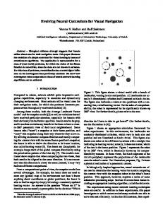
instead must discover which actions yields the most reward by trying them. Figure 1 shows the agent-environment interaction in reinforcement learning [1]. The Q-Learning algorithm proposed by Watkins, C. and Dayan, P. [2] is a widely used implementation of reinforcement learning based on dynamic programming technique and temporal difference methods [1]. The algorithm estimates the expected discounted numerical signal reward Q(s,a) by taking action a at state s. This will bring the robot to the next state, s’. The algorithm further estimates the numerical signal for the next state Q(s’,a’) assuming action a’ is taken in state s’. Then, using the results of each action, it updates the Q-values of the Q-table according to the following equation, Q(s, a ) ← Q(s, a ) + α [r + γ max a ' Q (s ' , a ') − Q(s, a )] (1)
where α is the learning rate, γ is the discount rate and r is the immediate reinforcement. The nature of the Q-learning algorithm towards problems with a discrete set of states and actions make it very suitable for the development of mobile robot navigation behavior such as obstacle avoidance and wall following.
Keywords—Reinforcement Learning, Neural QLearning, Fuzzy Logic, Obstacle Avoidance, Wall Following, Khepera II, Webots.
Agent reward rt
I. INTRODUCTION
A
S defined by Sutton, R. S. and Barto, A. G. [1], reinforcement learning is learning what to do - so as to maximize the numerical signal reward. The learner is not told which actions to take, as in most forms of machine learning, but
Velappa Ganapathy is with the School of Engineering, Monash University Sunway Campus, Jalan Lagoon Selaton, 46150 Banday Sunway (phone: +60-3-55146250; fax:+60-355146207; e-mail:
[email protected]). Wen Lik Dennis Lui., is with the School of Engineering, Monash University Clayton Campus, 3168 VIC Australia. (email:
[email protected]).
state st
action at rt+1 st+1
Environment
Fig. 1 The Agent-Environment Interaction in Reinforcement Learning
However, its original standard tabular formation used to hold Q-values would not yield an efficient system. For instance, a robot with eight sensors which has an input range of 0-1022 for each sensor with five actions to choose from will require a (1.1995 x 1024) x 5 Q-table. To
Department of Mechanical Engineering, Mepco Schlenk Engineering College, Sivakasi, India
behavior for the robot and its inputs are made up of the 8 proximity sensors. The other category of reinforcement learning controllers is the vision-based controllers. The previously discussed works are all sensor-based controllers. The most basic vision based controllers are those which directly input the captured image to the neural network. This is illustrated in the work of Iida, M. et al [9] and Shibata, K. and Iida, M. [10]. The former utilized a linear grayscale camera (1x64 pixels) and the latter utilized a CCD camera (320x240 pixels). The actor-critic architecture was utilized to enable the mobile robot to orientate itself towards an object and pushes it towards the wall. To further improve the behavior of vision based controllers, Gaskett, C. et al [11] had utilized a continuous state, continuous action reinforcement learning algorithm based on a multilayered feed-forward neural network combined with an interpolator. This interpolation scheme is known as ‘wire-fitting’. The ‘wirefitting’ function is a moving least squares interpolator which is used to increase the speed experienced during the Q-value updating process. It allows the updating process to be conducted whenever it is convenient. The simulation results show that the robot is capable of demonstrating wandering and servoing behaviors through trial and error using reinforcement learning.
efficiently update and read the Q-values from such a large table would impose a serious problem. The only was to learn anything at all on these tasks is to generalize from previously experienced states to ones that have never been seen. As such, the standard tabular formation had been replaced by function approximators such as neural networks. II. RELATED WORKS Apart from applying neural networks to Qlearning, it has also been applied onto actor-critic architectures. The types of neural network utilized for reinforcement learning algorithms are the backpropagation feed-forward neural network, recurrent neural network and the self organizing maps. Jakša, R. et al [3], Yang, G.-S. et al [4] and Huang, B.-Q. et al [5] had similarly approached the problem of mobile robot navigation through the combination of the multilayer feed-forward neural network with reinforcement learning algorithms. Jakša, R. et al [3] had utilized an actor critic architecture whereas the latter two had utilized the Q-Learning algorithm. All results obtained are verified via simulation results only. In addition, the developed reinforcement learning controllers are entirely based on the mobile robots’ sensors. The main difference between the recurrent neural networks and the backpropagation feedforward neural networks is their internal structure. The input layer of the recurrent neural network is divided into two parts; the true input units and the context units. The context units simply hold a copy of the activations of the hidden units from the previous time steps. In 1998, Onat, A. et al [6] had thoroughly discussed the architecture, learning algorithms and internal representation of recurrent neural networks for reinforcement learning and had performed comparisons across the different types of network architectures and learning algorithms through a simple problem. At the same time, Cervera, E. and del Pobil, A.P. [7] had not only applied the recurrent neural network for a sensor-based goal finding task, but the duo extended it by proposing a new method for state identification that eliminates sensor ambiguities. The implementation of self organizing maps for Q-learning was further illustrated by Sehad, S. and Touzet, C. [8]. This network learns without the requirements of supervision and it could be able to detect irregularities and correlations in the input, and adapt to that accordingly. The pair had used the self organizing maps together with Qlearning to develop an obstacle avoidance
III. SYSTEM OVERVIEW Webots [12] is a commercial mobile robot simulation software used by over 250 universities and research centers worldwide to model, program and simulate mobile robotics. The main reason for its increasing popularity is due to its ability to reduce the overall development time. Using this platform, a flexible simulation for the Khepera II was developed. Some of the notable features in the simulation are the custom maze design feature, repositioning and reorientation of the sensors, changing wall and floor textures, light intensities, etc. In addition, Webots was interfaced with the Microsoft Visual C++ .Net 2002 integrated development environment by using a combination of MC++, C++ and C programs. Furthermore, the C programs were interfaced to Matlab 7.1 through the Matlab engine. Matlab was further used to communicate to the serial port such that control commands could be sent to the real robot and vice-versa via the radio base and radio turret. The interaction of the various modules of system is shown in Fig. 2.
2
International Conference on Fascinating Advancement in Mechanical Engineering (FAME2008), 11-13, December 2008
Autodesk 3ds Max
Neural Network, Image Processing Tool Box
MC++ & C++ Supervisor MC++, C++ & C Controller
Matlab Session
Determine an action, a according to the Boltzmann Probability Distribution (during learning) or the equation a = max(Q(s,a)) (after learning). (vi) Robot takes action, a and reach a new position. Get current state. (vii) If a collision occurred, a negative numerical reward signal will be granted and the robot is reset back to its initial position. (viii) Then, generate Qtarget according to the equation:
(v)
Qt arget (st , at ) = r (st , at , st +1 ) + γ maxQ(st +1 , at +1 ) (2) at +1εA
DBots
where γ is the discount rate (0 ≤ γ ≤ 1), r (st , a t , s t +1 ) is the reward signal Cross-Compilation or Remote Connection
Simulation
Fig. 2 System Overview
The Neural Q-Learning algorithms are mostly written in C. It could be easily interchanged from one algorithm to another algorithm by using Graphical User Interface (GUI) developed for the robot controller. By treating Matlab as a background computation engine, the C programs are able to make use of the neural network toolbox in Matlab. Thus, data will be transmitted back and forth from the simulation to Matlab and vice-versa.
(ix)
(x)
assigned to action at for bringing the robot from state st to state st+1. Construct the error vector by using Qtarget for the output unit corresponding to the action taken and 0 for other output units. Repeat (iii)-(ix) until the robot is able to demonstrate the expected behavior.
To allow the mobile robot to explore the environment first and slowly converge to exploiting the learnt policy, the Boltzmann Probability Distribution was utilized. The Boltzmann probability could be denoted by the following equation,
IV. NEURAL Q-LEARNING In this work, a total of four controllers were developed. These controllers are:
prob(a k ) =
1 exp(Q (st , a k ) / Tt ) f
(3)
where (i) (ii) (iii) (iv)
Sensor-based Obstacle Avoidance Controller Sensor-based Wall Following Controller Vision-based Obstacle Avoidance Controller Obstacle Avoidance Controller based on a Combination of Sensor and Visual Inputs
A common learning algorithm applies to all these controllers. The Neural Q-Learning algorithm implemented is as follows, (i)
(ii) (iii)
(iv)
Initialize the neural network in Matlab and randomly assign the weights of the neural network. Define the initial position of the Khepera II in the simulation. Obtain the sensor readings from the infrared sensors/ visual input from the camera/combination of both. Obtain Q(s,a) for each action by substituting the current state and action into the neural network.
f = ∑ exp(Q(s t , a ) / Tt )
(4)
a
and t is the current iteration and k is the index of the action selected. The Boltzmann Probability Distribution was originally derived for physics and chemistry applications. Nevertheless, it was adopted for the use in reinforcement learning algorithms to define a policy which becomes greedier over time. The key parameter to ensure this policy is the T parameter, which is known as the temperature. It controls the randomness of the action selection by setting it high at the beginning of the learning phase and slowly decreasing on each iteration by the following equation,
Tt +1 = Tmin + β (Tt − Tmin )
(5)
Department of Mechanical Engineering, Mepco Schlenk Engineering College, Sivakasi, India
where Tmin and β (0 < β ≤ 1) are constants. Thus, as T approaches Tmin, the robot will change from exploration to exploitation of the learnt policy. The robot will have a total of 5 actions to select at any state. These actions are illustrated in Fig. 3.
B. Sensor-based Wall Following Controller This controller is basically an extension over the sensor-based obstacle avoidance RL controller. The network configurations and parameters used are the same for both controllers. The only difference between this and the previous controller is its reward function. By altering the reward function, the robot learns to refine its behavior from an obstacle avoidance behavior to a much refined wall following behavior. The reward function is designed as, Forward Motion: Turn Left: Turn Right: Rotate Left: Rotate Right:
Fig. 3 The Five Actions of the Khepera II
A. A Sensor-based Obstacle Avoidance Controller This controller is very much similar to the works of Yang, G.-S. et al [4] and Huang, B.-Q. et al [5]. However, they had only validated this in simulation only. In this work, it has been further extended to the validation of the controller on the actual robot. The input states are the 8 sensor readings. The neural network design which has successfully demonstrated the desired result is a 3 layer feed-forward backpropagation neural network. Fig. 4 shows the neural network architecture for this controller. It has 3 layers with 8 neurons on the input layer (pure linear activation function), 16 neurons on the hidden layer (tangent sigmoid activation function) and 5 neurons on the output layer (pure linear activation function). The Variable Learning Rate Backpropagation training algorithm is used to train the neural network and it has eight input which ranges from 0 to 1022 for each infra-red distance sensors. The reward function is designed as, Forward Motion: Turn Left: Turn Right: Rotate Left: Rotate Right:
+0.05 +0.00 +0.00 -0.10 -0.10
A collision is defined to take place when any one of the five front sensors reads a value exceeding 600. If so, the reward for that iteration is -10.00. However if the reading is in between 250-600, then the final reward obtained is +1.00. C. Vision-based Obstacle Avoidance Controller This controller represents its states in a totally different way if compared to the sensor-based controllers. The visual input is acquired from the K213 Linear Grayscale Camera. It provides an image with an array size of 1x64 pixels. To allow the robot to acquire an obstacle avoidance behavior through the linear grayscale input, some modifications are performed to the original environment. The surrounding wall textures will be required to be changed to black and white stripes. The number and width of these stripes changes as the robot moves toward or away from the walls. As such, this will serve as a pattern for the robot to determine whether it is close to a wall, based on the visual input. Fig. 5 shows the Khepera II with the K213 Linear Grayscale Camera Module.
+0.30 +0.15 +0.15 -0.10 -0.10
Fig. 4 Neural Network Architecture
Fig. 5 Khepera II with the K213 Linear Grayscale Camera
A collision is defined to take place when any one of the five front sensors reads in a value exceeding 600. If so, the reward for that iteration is -10.00.
Looking at the size of the input image, it suggests that if the image is to be applied directly to the neural network, the neural network will require 64 neurons on its input layer. However, via several experiments, it was found that the neural network was not able to generalize. Thus,
4
International Conference on Fascinating Advancement in Mechanical Engineering (FAME2008), 11-13, December 2008
the 64 grayscale values are divided into 8 segments, each containing 8 pixels. For each segment, the average grayscale value is calculated and fed to the neural network on each iteration. This conversion results in 8 average grayscale values for the 8 segments. Similarly, the neural network architecture shown in Fig. 4 could be applied to this controller. The reward function was designed similar to the sensor-based obstacle avoidance controller. D. Obstacle Avoidance Controller based on a Combination of Sensor and Visual Inputs This controller was proposed in order to overcome the weakness of the vision-based obstacle avoidance controller. Its weakness will be illustrated in the following section. This controller does not only avoid obstacles but it also stays away from black objects. This behavior is created by implementing a Fuzzy Logic Controller (FLC). The FLC fuzzifies the 8 sensor and 8 average grayscale values into 8 outputs. It is designed in such a way that the sensor readings take more priority over the visual input. For each input, three membership functions are specified i.e. low, medium and high. The membership functions for the sensor inputs are as illustrated in Fig. 6(a) and the membership functions for the averaged grayscale values of the linear grayscale image are as illustrated in Fig. 6(b).
(a)
(b)
Fig. 6 Membership Function for (a) Sensor Readings and (b) Averaged Grayscale Values
As there are 8 sensors and 8 averaged grayscale values, the rules are relatively easy to define. The combination of the sensor input and image segment will totally depend on its position. For example, sensor ds0 which is located on the left side of the Khepera will be combined with the averaged value of the left most segment of the grayscale image. For the last two averaged values, there are no other options but to pair it with the two rear sensors. However, this is not to worry as the two readings from the rear sensors are normally not taken into consideration as there are no backward motions. Fig. 7 shows the membership function of the FLC outputs and the rules for each pair of inputs are as follows, • If (ds0 is high) then (output1 is high) (1)
• • • • •
If (ds0 is medium) and (a0 is medium) then (output1 is medium) (1) If (ds0 is medium) and (a0 is low) then (output1 is medium) (1) If (ds0 is low) and (a0 is high) then (output1 is high) (1) If (ds0 is low) and (a0 is medium) then (output1 is medium) (1) If (ds0 is low) and (a0 is low) then (output1 is low) (1)
Fig. 7 FLC Output Membership Function
The neural network architecture implemented for this controller is a 3 layer feed-forward backpropagation neural network. Likewise, it has 8 neurons on the input layer (pure linear activation function), but 32 neurons on the hidden layer (tangent sigmoid activation function) and 5 neurons on the output layer (pure linear activation function). The Variable Learning Rate Backpropagation training algorithm was utilized and its reward function is designed as, Forward Motion: Turn Left: Turn Right: Rotate Left: Rotate Right:
+0.50 +0.15 +0.15 -0.20 -0.20
A collision is defined to take place when any one of the five front sensors reads a value exceeding 600. If so, the reward for that iteration is -10.00. Then if the total number of inputs in the current state exceeding 200 is less than the total number of inputs in the next state exceeding 200, then the original numerical reward assigned for taking that action gets an additional 0.50. V. RESULTS AND DISCUSSION Before presenting the results of the controllers, there is a need to develop certain measures to evaluate the function approximator, which is the neural network in this case. Most supervised learning seeks to minimize the mean-squared error (MSE) over some distribution, P, of the inputs. Another measure is the number of epochs it takes the neural network to acquire a behavior. However, with this algorithm, it is very hard to ensure that a better approximation at some state can be gained without the expense of worse approximation at other states. This widely known
Department of Mechanical Engineering, Mepco Schlenk Engineering College, Sivakasi, India
issue is termed as the interference problem. As such, the most effective performance measure of the neural network performance is through observation of its actual behavior. Although this does not provide an accurate measure of its performance, however, it is the best way to ensure the function approximator had successfully acquired the desired behavior. Video clips of the robot were recorded for observation purposes. However, to illustrate the results in this paper, the trajectory taken by the robot in the simulated and actual environment will be drawn.
C. Vision-based Obstacle Avoidance Controller The results shown in Fig. 10 suggest that the neural network is able to generalize when the average grayscale values are fed into the neural network. Although the robot learns how to avoid colliding onto walls through the visual input, however, its limited field of view has resulted in side collisions. Due to this, the controller was not tested on the real robot to avoid unnecessary damage.
A. Sensor-based Obstacle Avoidance Controller It could be seen in Fig. 8 that the robot has successfully demonstrated an obstacle avoidance behavior. In the simulation, more obstacles are present. This is due to the convenience of the custom maze building feature in the supervisor controller program developed in Webots. However, for the real robot, the environment is made much simpler due to mobility issues. The learning time for each neural network which has its weights randomly assigned differs significantly. Thus, the number of epochs during each learning phase does not indicate anything at all.
(a)
D. Obstacle Avoidance Controller based on a Combination of Sensor and Visual Inputs This controller incorporates two behaviors with the same goal; the obstacle avoidance behavior together with the avoidance of dark object by implementing a FLC. To test this controller, black objects are placed on strategic locations on the walls which act as a secondary guide for the robot to reach its final position. The sensor readings keep it safe from wall collisions on the side. This makes this controller more superior to the visionbased controller. Fig. 11 shows the trajectory taken by the robot in both simulated and actual environment.
(b)
(a)
(b)
Fig. 10 Vision-based Obstacle Avoidance Controller (a) Simulation 1 and (b) Simulation 2
Fig. 8 Sensor-based Obstacle Avoidance Controller (a) Simulation Results and (b) Real Robot Results
B. Sensor-based Wall Following Controller The sensor-based wall following behavior was successfully acquired by the robot and the results are illustrated in Fig. 9. As compared to the previous controller, the movement of the robot is much more refined. This is because the robot travels following the position of the walls. To achieve this behavior will only require slight modifications in the reward function.
(a)
(b)
(c) (a)
Fig. 11 Obstacle Avoidance Controller based on Combination of Sensor and Vision Inputs (a) Simulation Results, (b) Real Robot Results 1, (c) Real Robot Results 2
(b)
Fig. 9 Sensor-based Wall Following Controller (a) Simulation Results and (b) Real Robot Results
6
International Conference on Fascinating Advancement in Mechanical Engineering (FAME2008), 11-13, December 2008
E. Discussion The main advantage of reinforcement learning is its ability to allow the robot to learn through interaction. The environment can be totally unknown. It learns through the rewards it obtains for each action taken under different states. This concept is similar to how humans learn. Humans learn naturally through experience. For example, we learn not to touch a cactus after we get our fingers pricked. The pain has resulted in a negative reward. As such, through an accumulation of different experiences, humans acquire new skills and behavior. Of course, for the case of reinforcement learning controller, it will require further advances in its theory before it could reach such levels. The drawback about the learning algorithm is the large amount of unknowns. All the parameters such as the discount rate, initial temperature parameter, reward function and neural network parameters are unknowns. There are no formulas or guidelines to select an optimum set of parameters for the problem at hand. This has resulted in a major drawback when different configurations are being experimented. Performing analysis on the neural network is already complex enough but the additional parameters introduced by the learning algorithm makes the analysis even tougher. Due to large number of parameters which could be altered, it is often quite hard to identify the actual reason for the failure of the robot to learn a desired behavior. The only way to identify how these parameters influence the system is through experience. Experimental results reveal that the discount rate should always start from a lower value such that the neural network, which has its weights randomly assigned, could settle down to an equal state before the actual learning phase starts. Then, the discount rate is slowly increased as the number of iteration increases. Furthermore, it was found that the Variable Rate Learning Backpropagation training algorithm works well for the value approximation problem. Another major drawback with this algorithm is the presence of the interference problem. One approach to this problem is to adopt the SemiOnline Neural Q-Learning algorithm [13]. This network acts locally and assures that learning in one zone does not affect the learning in other zones. It uses a database of learning samples. The main goal of this database is to include a representative set of visited learning samples, which is repeatedly used to update the Neural QLearning algorithm. The immediate advantage of this is the stability of the learning process and its convergence even in difficult problems. All the samples in the database will be compared to the new ones. If the old ones are found similar to the
new ones, they will be replaced. This ensures that the database is maintained at the optimum size and no extra unnecessary training time is taken p due to duplicate samples. However, there are still issues regarding the training required for each training cycle when the database scales up. Furthermore, an efficient updating procedure is required for the database such that minimum time is required for the updating process. VI. CONCLUSION In this paper, four reinforcement learning controllers based on the Neural Q-Learning algorithm were designed and tested on the actual and simulated robot using the Webots Commercial Robot Simulation software. In addition to building a flexible simulation environment for the Khepera II, further extension was made to the work by Yang, G.-S. et al [4] and Huang, B.-Q. et al [5] by validating the sensorbased obstacle avoidance controller on the actual robot. This eventually leads to the investigation of the wall following behavior and vision based controllers with the pros and cons of the learning algorithm observed during experiments being highlighted. In conclusion, the robot was able to acquire its desired behavior through its interaction with the environment. ACKNOWLEDGMENT The authors thank Monash University Malaysia for the support of this work. REFERENCES [1] [2] [3]
[4]
[5]
[6]
[7]
Sutton, R.S. and Barto, A.G., “Reinforcement Learning: An Introduction”, MIT Press, 1998. Watkins, C. and Dayan, P., “Q-Learning”, Machine Learning, vol.8, pp.279-292, 1992. Jakša, R., Sinčák, P. and Majerník, P., “Backpropagation in Supervised and Reinforcement Learning for Mobile Robot Control”, Available: http://neuron-ai.tuke.sk/~jaksa/publication s/JaksaSincak-Majernik-ELCAS99.pdf (Accessed: 2006, April 24). Yang, G.-S., Chen, E.-K. and An, C.-W., “Mobile Robot Navigation Using Neural Q-Learning”, Proceedings of 2004 International Conference on Machine Learning and Cybernetics, vol. 1, pp. 48-52, 2004. Huang, B.-Q., Cao, G.-Y. and Guo, M., “Reinforcement Learning Neural Network to the Problem of Autonomous Mobile Robot Obstacle Avoidance”, Proceedings of 2005 International Conference on Machine Learning and Cybernetics, vol.1, pp. 85-89, 2005. Onat, A., Kita, H. and Nishikawa, Y., “Recurrent Neural Networks for Reinforcement Learning: Architecture, Learning Algorithms and Internal Representation”, 1998 IEEE International Joint Conference on Neural Networks Proceedings, vol. 3, pp. 2010-2015, 1998. Cervera, E. and del Pobil, A.P., “Eliminating Sensor Ambiguities Via Recurrent Neural Networks in SensorBased Learning”, 1998 IEEE International Conference
Department of Mechanical Engineering, Mepco Schlenk Engineering College, Sivakasi, India
[11] Gaskett, C., Fletcher, L. and Zelinsky, A., “Reinforcement Learning for a Vision Based Mobile Robot”, Available: http://users.rsise.anu.edu.au/~rsl/r sl_papers/2000iros-nomad.pdf (Accessed: 2006, May 31). [12] Webots. http://www.cyberbotics.com. Commercial Mobile Robot Simulation Software. [13] “Semi-Online Neural-Q Learning”, Available: http://www.tdx.ce sca.es/TESIS_UdG/AVAILABLE/TDX-0114104123825//tm cp3de3.pdf (2006, June 30).
on Robotics and Automation, vol. 3, pp. 2174-2179, 1998. [8] Sehad, S. and Touzet, C., “Self-Organizing Map for Reinforcement Learning: Obstacle-Avoidance with Khepera”, Proceedings from Perception to Action Conference, pp. 420-423, 1994. [9] Iida, M., Sugisaka, M. and Shibatam K., “Application of Direct-Vision-Based Reinforcement Learning to a Real Mobile Robot”, Available: http://shws.cc.oitau.ac.jp/~shibata/pub/ICONIP02-Iida.pdf (Accessed: 2006, June 24). [10] Shibata, K. and Iida, M., “Acquisition of Box Pushing by Direct-Vision-Based Reinforcement Learning”, Available: http://shws.cc.oita-u.ac.jp/~shibata/pub/SIC E03.pdf (Accessed: 2006, June 24).
8