IUCAA-14/2016 LIGO-P1600094
Transient Classification in LIGO data using Difference Boosting Neural Network N Mukund,1, a S Abraham,1, b S Kandhasamy,2, c S Mitra,1, d and N S Philip3, e
arXiv:1609.07259v3 [astro-ph.IM] 9 May 2017
1
Inter-University Centre for Astronomy and Astrophysics (IUCAA), Post Bag 4, Ganeshkhind, Pune 411 007, India 2 The University of Mississippi, University, Mississippi 38677, USA 3 Department of Physics, St. Thomas College, Kozhencherry, Kerala 689641, India (Dated: May 10, 2017) Detection and classification of transients in data from gravitational wave detectors are crucial for efficient searches for true astrophysical events and identification of noise sources. We present a hybrid method for classification of short duration transients seen in gravitational wave data using both supervised and unsupervised machine learning techniques. To train the classifiers we use the relative wavelet energy and the corresponding entropy obtained by applying one-dimensional wavelet decomposition on the data. The prediction accuracy of the trained classifier on nine simulated classes of gravitational wave transients and also LIGO’s sixth science run hardware injections are reported. Targeted searches for a couple of known classes of non-astrophysical signals in the first observational run of Advanced LIGO data are also presented. The ability to accurately identify transient classes using minimal training samples makes the proposed method a useful tool for LIGO detector characterization as well as searches for short duration gravitational wave signals.
Detection of short duration gravitational waves (GW) in LIGO data requires reliable identification and removal of noise transients produced by variety of nonastrophysical sources [1, 2]. Noise transients present in the data reduces the reliability of a GW detection by increasing its false alarm probability. Mitigation of noise transients is a major challenge in searches for GW, specially for short duration events where the signal can be easily mimicked by non-astrophysical transients of varied origin. These often have waveform morphology close to that of the targeted signal, thus making the differentiation even more difficult [3]. With the advent of big data analysis, machine learning has emerged as a useful tool to handle huge volumes of data and to interpret meaningful results from them. In the past few decades, machine learning algorithms such as Artificial Neural Network (ANN) [4, 5], Support Vector Machines [6, 7], Random Forest [8], Gaussian Mixture Model [9] etc. found many applications in astronomy and occasionally have been used for the study of noise artefacts in GW analysis. Since the visual inspection of individual events and their classification is time consuming and prone to errors, machine learning methods are more effective and reliable for the detection of hidden signatures of astrophysical GW in the data. We present a hybrid classifier that combines features from supervised and unsupervised machine learning algorithms to do the transient classification. Our classifier performs an unsupervised hierarchical clustering on the incoming data to identify possible groups and a supervised Bayesian [10] classifier to do the final classification. The classifier code uses features extracted from wavelet
a b c d e
[email protected] [email protected] [email protected] [email protected] [email protected]
analysis of the data in a fast and efficient manner using GPU and MPI parallelization techniques, whereby, making it a good candidate for real-time burst trigger classification and detector characterization. When used to predict the class labels for an input data, the classifier ranks the most likely classes each with an associated probability (confidence level) that may be used to set a threshold to discard unreliable predictions. This multiple class prediction is useful to identify borderline examples in the feature space. In our study, the classifier was first tested on simulated data consisting of astrophysical bursts along with commonly observed instrumental glitches and then on the LIGO sixth science run burst hardware injections. Targeted searches for specific glitch types seen in Advanced LIGO first observation data were also carried out and the results are reported. Recent methods like deep learning [11, 12] using convolutional neural networks require large number of training data and are computationally expensive. The fact that we are able to represent the transient classes with minimal features and fewer training data samples makes our method less susceptible to such issues and speeds up the training process, making it suitable for realtime applications.
I.
TRANSIENT EVENTS IN GW DATA
Table I lists the transients used in our analysis. Standard searches for compact binary coalescences use matched filtering as the base algorithm [13], while the burst searches primarily look for excess power in the data along with time coincidence to trigger a detection [14, 15]. Both these searches are followed by extensive sanity checks, where the auxiliary channels insensitive to astrophysical signals are inspected to rule out possible terrestrial coupling [3]. Auxiliary channels are often in thousands and their coupling with the GW strain sensitive channel is seen to fluctuate in time due to the dynamic nature of the instrument. This often makes
2 the auxiliary channel veto procedure a daunting task. Incorporating a machine learning based veto procedure to identify well known classes of non-astrophysical transients can help discern the trigger right at the strain channel and thus reduce false alarms.
II.
CLASSIFIER
Machine learning involves techniques which allow systems to automatically learn and improve prediction accuracies by exploring their past experiences on data. It mimics human decision-making ability by discovering the relationships between the variables of a system from a given set of examples that have both the variables and the observed outcomes. Here we use a hybrid classifier, a supervised Bayesian [10] one called Difference Boosting Neural Network (DBNN) [16, 17], to classify the burst signals. The DBNN can impose conditional independence on data without loss of accuracy in the posterior computations. It does this by associating a threshold window with each of the attribute values of the examples [18]. The network is designed to work with discrete value input features while GW data features are continuous. A simple method to deal with continuous feature value is to recast it into a suitable number of bins. There is no fixed criteria for the number of bins each feature may take. It might be argued that smaller the bin size, conditions can be imposed with better accuracy. However, in most practical situations, the optimal bin size is close to the square root of N, where N represents the number of discrete values present in the data for that variable. Once the bins are defined, for each feature bin and the given classes, the allowed ranges for all the remaining features are registered. The DBNN, being a supervised neural network, requires a training data to configure the network before it can be used for classification of unseen data. The learning takes place by highlighting the difference between the features in two or more classes [18] by using Bayesian probability as its central rule for decision making. The confidence in a prediction [19] is the value of the posterior Bayesian probability for a given set of input features. The working of DBNN can be divided into three units: Bayesian Probability Estimator, Gradient Descent Boosting Algorithm, and a Discriminant Function Estimator [18]. The network starts with a flat prior for all the classes P (Ck ) = 1/N , preventing the training from being biased to any specific prior distribution. The first unit in DBNN (executed by option 0 in the implementation) computes Bayesian probability and the threshold function for each of the training sample by constructing a grid for each class with columns representing the attributes and rows their respective values. The bin location for each attribute value is decided such that the full range of values can be uniformly covered by the set number of bins for that attribute across the classes. Initially the content
in attribute bins are all set to one. The training examples are taken one by one and the bin corresponding to each attribute value for it’s class is incremented by one. This sampled data is used to compute the likelihood for an attribute value to favour a class, P (Um |Ck ), as the ratio of occurrences (counts) in it’s bin for the class CK to the total counts in all k classes for the same bin number that Um holds for that attribute. The classifier also makes notes for each attribute value and it’s class, the allowed maximum and minimum values taken by the remaining attributes in the entire training sample. This information is used to negate the possibility that the value of one feature may favour multiple classes, unless all other features also have values in the same range across the classes. Though we started with a flat prior, to compute the Bayesian probability, we need to estimate the actual prior. In the Bayesian framework, prior has no special meaning. It is a weighted bias (belief) about the probable outcome of an experiment based on experiences in the past. In the second unit (executed by option 1 in the implementation), the DBNN estimates prior based on it’s experience with the given training data. The DBNN does not make any change in the prior for correctly classified examples. In the case of failed examples, it attaches an additional weight to the attributes so that, it may also get correctly classified. To avoid random fluctuations due to the introduction of arbitrary priers, this is done by modifying the flat prior incrementally by ∆Wm = α(1 − PPkk∗ ) through a set of repeated rounds on the training data until the example gets correctly classified. That is, until P (U |Ck ) = Πm P (Um |C) goes to a maximum for the true class represented by the data. Here Pk and Pk∗ respectively represent the calculated Bayesian probability for the true class and the wrongly estimated class and α is a fraction called the learning rate [19]. Since ratio of the probabilities are taken, this is much like the way humans arrive at their priers based on their cumulative experiences in the past. This process is called training, and after training, the estimated likelihoods and prior are saved for future use. The assumption during the training process is that a representative training data is available that has suitable examples to represent all the variants in the target space. The third unit (executed by option 2 and 3 in the implementation) computes the discriminant function. According to Bayesian theorem, the updated belief or the posterior is the product of the prior and the evidence normalised over all possibilities. This can be written as Q m (P (Um |Ck )Wm P (Ck |U ) = P Q (1) k m (P (Um |Ck )Wm where Wm represent the prior weight vector. DBNN has been successfully applied to many astronomical problems such as star-galaxy classification [18], classification of point sources such as quasars, stars and unresolved galaxies [20], transient classification [21] to indicate a few.
3
Normalized Amplitude
RD
1.0
0.6
0.6
0.6
0.2
0.2
0.2
0.2
0.2
SN
1.0 0.6
0.6
0.2
0.2
0.2 1.2
CSP
1.0
0.20
GA
1.0
WNB
0.8 0.4 0.0
0.2
0.2
LBM
1.0 0.6
0.8
CSG
1.0
Blip
0.6
0.6
0.05 0.00
0.00
0.4 0.0
0.4
0.5
0.6
0.7
0.3
0.4
0.5
0.6
0.7
GA
0.0
CSP
0.0
CSG
0
2
4
6
8
10 12 14
Time [sec]
BLIP
0.8
0.4
0.0
WBN
0.8 0.4
0.0 0.8
LBM
0.8
0.2
0.3
0.2
0.4
0.04
0.4
0.7
0.2
0.8
0.08
0.2 0.6
SN
0.12
0.2
0.5
0.6 0.4
0.0
0.16
0.2 0.4
RD
0.4
0.10
0.2
0.3
0.6
SG
0.15
Detailed Coefficient Wavelet Energy
SG
1.0
0.4 0
2
4
6
8
10 12 14
Wavelet Energy Levels
0.0
0
2
4
6
8
10 12 14
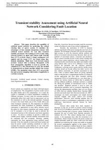
FIG. 1. Left panel depicts typical transient events (SNR set to 50 for better visualisation). Wavelet energy median distribution for simulated data (SNR varied from 8 to 100) shown in the right panel .
Hierarchical Clustering
Observed Triggers
16
14
12
Height
10
8
Time Series Whitening Simulated Triggers
Multilevel 1D Wavelet Decomposition
Detail Coefficient Energy & Wavelet Entropy Computation
Hierarchical Clustering to Identify Dominant Transients
Optimal Class Selection for Supervised Learning
6
4
DBNN Testing
DBNN Training
Real Time Input Triggers
> 2
Wavelet-DBNN Classifier
> 0
FIG. 2. Dendrogram showing hierarchical clustering of 1000 transient triggers identified in O1 Data from Hanford observatory by the Omicron algorithm [22]. The transient morphology changes progressively from left to right
As for the case of all supervised networks, the accuracy of the predictions depend on the initial class selection and quality of the training data sets. When encountering real instrument data where it is difficult to know beforehand the actual groups present, running an unsupervised classifier prior to Wavelet-DBNN classifier was seen to vastly improve the results. This step becomes more relevant for targeted searches looking for a particular transient class where unsupervised learning can yield insights into contamination from other glitch classes. Prior information about other glitches with very similar morphology can be made use of by the network to learn to differentiate between them whereby improving the accuracy.
Hierarchical Clustering of Unidentified/Rejected/Low confidence Transients
Classified Trigger List
FIG. 3. Block diagram of the proposed hybrid classifier.
We run an unsupervised classifier using Hierarchical clustering on the data to get an idea about the possible transient groups currently present in the data and their respective distribution (see Figure 2). Classifier trained this way is observed to outperform the other scenarios where class selection is done either by visual inspection or by using predefined classes. We employ a bottom up agglomerate clustering where the pairwise distance is calculated using Mahalanobis distance measure [23]. The criterion for estimating the linkage between the clusters is based on the average distance between pairs of signals among the clusters, weighted by the numbers of elements in each cluster. Cluster linkage at each level of dendrogram is calculated recursively
4 whose value for a given pair of clusters is given by
s d(r, s) =
2nr ns k˜ xr − x ˜s k2 (nr + ns )
III.
(2)
The optimal distance measure used for linkage and the original mother wavelet used for decomposition are both selected based on the value of cophenetic correlation coefficient,c [24] with value close to unity being ideal.
P
(Yij − y)(Zij − z)
i