Automatic Microstructural Characterization and Classification using ...

Automatic Microstructural Characterization and Classification using Artificial Intelligence Techniques on Ultrasound Signals Thiago M. Nunesa , Victor Hugo C. de Albuquerqueb , João P. Papac , Cleiton C. Silvad , Paulo G. Normandoa , Elineudo P. Mourad , João Manuel R. S. Tavarese a

Departamento de Engenharia de Teleinform´ atica, Universidade Federal do Cear´ a, Fortaleza, Cear´ a, Brazil. Emails: [email protected], [email protected] b Programa de P´ os-Gradua¸c˜ ao em Inform´ atica Aplicada, Universidade de Fortaleza, Fortaleza, Cear´ a, Brazil Email: [email protected] c Departamento de Ciência da Computa¸c˜ ao, Universidade Estadual Paulista, Bauru, S˜ ao Paulo, Brazil. Email: [email protected] d Departamento de Engenharia Metal´ urgica e de Materiais, Universidade Federal do Cear´ a, Fortaleza, Cear´ a, Brazil. Emails: [email protected], [email protected] e Instituto de Engenharia Mecˆ anica e Gest˜ ao Industrial, Departamento de Engenharia Mecˆ anica, Faculdade de Engenharia, Universidade do Porto, Porto, Portugal. Email: [email protected]

Abstract Secondary phases such as Laves and carbides are formed during the final solidification stages of nickel based superalloy coatings deposited during the gas tungsten arc welding cold wire process. However, when aged at high temperatures, other phases can precipitate in the microstructure, like the γ ′′ and δ phases. This work presents a new application and evaluation of artificial intelligent techniques to classify (the background echo and backscattered) ultrasound signals in order to characterize the microstructure of a Ni-based alloy thermally aged at 650 and 950 °C for 10, 100 and 200 hours. The background echo and backscattered ultrasound signals were acquired using transducers with frequencies of 4 and 5 MHz. Thus with the use of features extraction techniques, i.e., detrended fluctuation analysis and the Hurst method, the accuracy and speed in the classification of the secondary phases from ultrasound signals could be studied. The classifiers under study were the recent Optimum-Path Forest (OPF) and the more traditional Support Vector Machines and Bayesian. The experimental results revealed that the Preprint submitted to Expert Systems with Applications

October 22, 2012

OPF classifier was the fastest and most reliable. In addition, the OPF classifier revealed to be a valid and adequate tool for microstructure characterization through ultrasound signals classification due to its speed, sensitivity, accuracy and reliability. Keywords: Feature Extraction, Detrended Fluctuation Analysis and Hurst Method, Optimum-Path Forest, Support Vector Machines, and Bayesian Classifiers, Non-destructive Inspection, Nickel-based Alloy, Thermal Aging. 1. Introduction Nb-bearing nickel-based superalloys, like the Inconel 625 alloy studied here, exhibit an outstanding combination of mechanical properties and resistance to pitting, crevice and intergranular corrosion due to the stiffening effect of chromium, molybdenum and niobium in its nickel matrix. These properties make precipitation hardening treatments unnecessary [1]. The extraordinary resistance against a wide range of organic and mineral acids is due to their excellent anti-corrosive properties, mainly at high temperatures. These alloys are commonly found in the marine, aerospace, chemical and oil and gas industries [2, 3, 4]. The Inconel 625 alloy in particular has greater applicability, especially in highly corrosive environments such as the oil and gas industry, than many other Nickel (Ni) based alloys. Nowadays, this alloy is used widely in the weld overlay of the inner surface of carbon steel pipes and other equipment for the offshore industry. However, further studies of this alloy, such as this paper, are necessary to increase the overall knowledge of its properties. During welding of an Inconel 625 alloy, there is an intensive microsegregation of some elements, such as Niobium (Nb) and Molybdenum (Mo), within the interdendritic regions, causing the supersaturation of the liquid metal with these chemical elements in its final stage of solidification, which results in the precipitation of Nb-rich Laves phase and MC primary carbides of type NbC [5, 6]. This segregation and precipitation of the secondary phases can change the mechanical properties of the alloy and decrease its resistance to corrosion [7]. In addition, the Nb-rich Laves phase has a low melting point that causes an increase in the temperature solidification range, making the alloy susceptible to solidification cracking [8]. However, an adequate selection of the welding conditions can minimize the formation of the Nb-rich Laves phases and consequently, reduce its susceptibility to solidification cracking. 2

Therefore, it is also important to investigate the phase transformation process. Nowadays, researchers are evaluating the use artificial intelligence techniques to characterize microstructures. For example, Albuquerque et al. [9] quantified the porosity of synthetic materials from optical microscopic images successfully, and the solution proposed, which was based on an Artificial Neuronal Network (ANN), proved to be more reliable. Albuquerque et al. [11]characterized the microstructures in images of nodular, grey, and malleable cast irons using a Multilayer Perceptron Neuronal Network (MLP) [10], Kohonen’s self-organizing artificial neuronal network [11], and using Optimum-Path Forest (OPF) classifier [12]. To evaluate the microstructures of hypoeutectic white cast iron accurately, morphological operators together with an MLP neuronal network [13] were necessary. However, the application of this techniques are not combined with non-destructive tests (i.e, ultrasound inspection), this being one of the main innovations of this work. However, despite the above mentioned techniques, improved classification methods for microstructural characterization are still required. To the best of our knowledge, this work introduces the fast, robust and recent OPF classifier, for first time to characterize and classify the microstructure of a thermally aged Ni-based alloy and in the as-welded state. This recent graphbased classifier reduces the pattern recognition problem as an Optimum-Path Forest computation in the feature space induced by a graph, [14]. As such, the OPF classifier does not interpret the classification task as a hyperplane optimization problem as traditional classifiers, but as a polynomial combinatorial optimum-path computation from some key samples, designated as prototypes, to the remaining nodes. A detailed description of the OPF classifier will be carried out in section 2.5.1. Therefore, the main goal of this work was to evaluate the competence of the OPF classifier to monitor, thought ultrasound signal classification, the kinetics of the phase transformation of a Ni-based alloy thermally aged at 650 and 950 °C for 10, 100 and 200 hours, as well as in the as-welded state. Detrended-fluctuation analysis (DFA) and Hurst method (Rescaled range RS) were used in the feature extraction phase (i.e., preprocessing). Raw data (original) and preprocessed ultrasonic background echo and backscattered signals acquired with two types of transducers (4 and 5 MHz) were considered. For a further assessment of the OPF efficiency, the results obtained were compared with the ones achieved using the powerful classifiers, in particular the SVM and Bayesian classifiers. 3

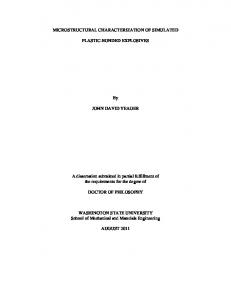
The potentiality and efficiency of ultrasonic signals combined with artificial intelligence classifiers to characterize the microstructures of a Ni-based alloy thermally aged and in the as-welded state were confirmed by the results. As far as the authors know, this is the first time that the effect of thermal aging on a Ni-based alloy has been analyzed using such classifiers on ultrasonic signals, which makes the results presented and discussed of noteworthy value. This paper is organized as follows: in the next section, the experimental procedures are described; then, in the third section, the experimental results are presented and discussed; finally, in the fourth and last section, the conclusions are pointed out. 2. Experimental Procedures This section describes the experimental work done to the temperatures 650 and 950 °C for 10, 100 and 200 hours, as well as the as-welded condition. First; the test setup is described, then the preparation of the Inconel 625 alloy samples is addressed. Afterwards, the ultrasonic signals acquired and the related fundamentals are introduced. Finally, the features extraction methods and artificial intelligence techniques used to process and classify the ultrasonic signals are presented. 2.1. Test setup Inconel 625 alloy coatings deposited on an ASTM A36 steel metal base were used in the experiments. The chemical compositions of these materials are given in [15]. For the welding a 4 mm diameter tungsten electrode doped with thorium was used, and pure argon (99.99%) was chosen as the shielding gas. An electronic multi-process power source connected to the data acquisition system monitored the current and tension during the welding. The manipulation of the torch was carried out using an industrial robot system, Figure 1(a). An automatic cold wire feed system for gas tungsten arc welding (GTAW) was used to supply the filler metal. Figure 1(b) shows the positioning unit that was used to guide the wire into the arc. This unit allows adjustments to be made to the configuration parameters and geometry of the wire feed. The weld coating was applied on an ASTM A36 steel metal base plate, resulting in a coating of 350×60×14 mm3 . The remaining welding parameters used were: 285 A of welding current (DCEN), arc voltage 4

of 20 V, travel speed equal to 21 cm/min, welding heat input of 16 kJ/cm, the wire feed speed equal to 6.0 m/min, arc length of 10 mm, 15 l/min of gas flow and arc oscillation describing a double-8 trajectory. Other minor considerations included the wire feed direction ahead of the arc weld, wire tip to pool surface was kept at a distance of 3 mm, the wire feeding angle was maintained constant and equal to 50°, and the electrode tip angle was fixed at 50°. To guarantee good overlaying with multiple passes deposited side by side, a distance equal to 2/3 of the initial weld bead width was established as an ideal step. Other arc oscillating parameters were: oscillation amplitude of 8 mm and wave length equal to 1.2 mm. To produce a 10 mm thick coating on the substrate, seven layers with eight passes were deposited under identical welding conditions.

(a)

(b)

Figure 1: Experimental setup used in the welding process: (a) robotic system, (b) GTAW guide wire feed and torch.

2.2. Samples preparation After the welding, the coating was detached from the substrate by conventional machining, as the material of interest was only the Inconel 625 alloy. Then, the coating was divided into seven samples; three samples were submitted to heat aging treatments at 650 °C, three at 950 °C and both for aging times of 10, 100 and 200 h [16], and the remaining one was kept as the as-welded state (0 h). The aged samples were water cooled with moderate agitation at room temperature. 5

Afterwards, the seven samples were subjected to metallographic preparation that included grinding, polishing and electrolytic etching using 10% chromic acid with a tension of 2 V tension for 15 seconds. Metallographic images were acquired using a scanning electron microscope (SEM) Philips XL30 (Oxford Instruments, England), and a study of the chemical composition of the secondary phases was carried out through energy dispersive spectroscopy of X-rays (EDS). After the microstructural analysis, the background echo and backscattered signals were acquired to evaluate the effect of aging on the Inconel 625 alloy samples. 2.3. Ultrasound signal acquisitions The pulse echo technique and direct contact method were used to capture the background echo and backscattered ultrasonic signals, [25]. All the signals were obtained using commercial NDT ultrasonic transducers: one of 4 MHz (Krautkramer, Germain, model MB4S) and another one of 5 MHz (Krautkramer, Germain, model MSW-QCG). The choice of these transducers was based on the authors previous experience in this kind of NDT and knowledge concerning the materials under study [17, 18, 19]. In fact, Albuquerque et al., in [15], showed that these frequencies revealed to be the most adequate to analyze the material under study, as a transducer with a frequency of 10 MHz completely attenuated the ultrasound signal, and one with a frequency of 2.25 MHz led to an adjacent echo that overlapped the signal extensively, seriously compromising the accuracy of the results. As a coupling material, SAE 15W40 lube oil was used for the longitudinal measurements. A Krautkramer ultrasound device (GE Inspection Technologies, USA, model USD15B) was used connected to a 100 MHz digital oscilloscope (Tektronix, USA, model TDS3012B), which transmitted the ultrasonic signals to a computer for processing, using a sampling rate of 1 GS/s. 2.4. Ultrasonic signal preprocessing and classification The microstructural characterization was carried out using OPF, Bayesian, SVM with Radial Basis Function (RBF), linear and polynomial kernels classifiers on the original background echo and backscattered signals. These signals were also preprocessed using feature extraction techniques based on detrended fluctuation analysis (DFA) and Rescaled method (RS), in which a better description of these methods can be found in [15]. In order to assure statistical significance, 40 signals were acquired for each sample and each 6

background echo signal had 10,000 points, i.e., a total of 400,000 points was attained, and each backscattered signal had 500 points, resulting in a total of 20,000 points for this study. After signal preprocessing using the DFA and RS techniques, the number of points of the background echo signals was reduced to 1680, i.e., a reduction of 42 times, the backscattered signals to 960 points, which means a reduction of 24 times. Albuquerque et al., in [15] did not consider echo signals without preprocessing, claiming that the large number of points made their use impracticable. However, this problem has been overcome because the classifiers used in this work are faster and more powerful, which is one of the important contributions attained with this work. 2.5. Ultrasound signals classification for the microstructural characterization In order to classify the original and preprocessed ultrasonic signal data, OPF, Bayesian, SVM RBF, SVM linear and SVM polynomial classifiers were employed and compared. For all classifiers, the training and testing phases were computed using the 10-fold cross validation approach on the same folds. For comparison purposes, the mean and standard deviation were computed on the results obtained by each classifier. 2.5.1. Optimum Path Forest classifier The OPF classifier models the problem of pattern recognition as a graph partition in a given feature space. The nodes are represented by the feature vectors and all pairs are connect by edges, defining a complete graph. This kind of representation is straightforward, given that the graph does not need to be explicitly represented, and has low memory requirements. The partition of the graph is carried out by a competition process between some key samples, known as prototypes, which offer optimum paths to the remaining nodes of the graph. Each prototype sample defines its optimum-path tree (OPT), and the collection of all OPTs defines the optimum-path forest, which gives the name to the classifier [14]. The OPF can be seen as a generalization of the well known Dijkstra’s algorithm to compute optimum paths from a source node to the remaining ones [20]. The main difference relies on the fact that OPF uses a set of source nodes, i.e., the prototypes, with any path-cost function. In case of Dijkstra’s algorithm, a function that summed the arc-weights along a path was applied. For OPF, a function that gives the maximum arc-weight along a path is used, [14]. 7

Let Z = Z1 ∪ Z2 be a dataset labeled with a function λ, in which Z1 and Z2 are, respectively, training and test sets, and let S ⊆ Z1 be a set of prototype samples. Essentially, the OPF classifier builds a discrete optimal partition of the feature space such that any sample s ∈ Z2 can be classified according to this partition. This partition is an optimum path forest (OPF) computed in ℜn by the image foresting transform (IFT) algorithm [21]. The OPF algorithm may be used with any smooth path-cost function which can group samples with similar properties [21]. This work used the path-cost function fmax , which is computed as: { 0 if s ∈ S, fmax (⟨s⟩) = +∞ otherwise. fmax (π · ⟨s, t⟩) = max{fmax (π), d(s, t)}, (1) in which d(s, t) means the distance between samples s and t, and a path π is defined as a sequence of adjacent samples. As such, fmax (π) computes the maximum distance between adjacent samples in π, when π is not a trivial path. The OPF algorithm assigns one optimum path P ∗ (s) from S to every sample s ∈ Z1 , originating an optimum path forest P (a function with no cycles which assigns to each s ∈ Z1 \S its predecessor P (s) in P ∗ (s) or a marker nil when s ∈ S. Let R(s) ∈ S be the root of P ∗ (s) that can be reached from P (s). The OPF algorithm computes for each s ∈ Z1 , the cost C(s) of P ∗ (s), the label L(s) = λ(R(s)), and the predecessor P (s). The OPF classifier is composed of two distinct phases: (i) training and (ii) classification. The former step consists, essentially, of finding the prototypes and computing the optimum-path forest, which is the union of all OPTs rooted at each prototype. After that, a sample is picked from the test sample, which is connect it to all the samples of the optimum-path forest generated in the training phase. Notice that this test sample is not permanently added to the training set, i.e., it is used only once. The next sections describe this procedure in more detail. Training. We say that S ∗ is an optimum set of prototypes when the OPF Algorithm minimizes the classification errors for every s ∈ Z1 . S ∗ can be found by exploiting the theoretical relation between the minimum-spanning tree (MST) and optimum-path tree for fmax [22]. The training essentially consists of finding S ∗ and an OPF classifier rooted at S ∗ . 8

By computing an MST in the complete graph (Z1 , A), we obtain a connected acyclic graph whose nodes are all samples of Z1 and the arcs are undirected and weighted by the distances d between adjacent samples. The optimum spanning tree is the tree that has the least sum of its arc compared to any other spanning tree in the complete graph. In the MST, every pair of samples is connected by a single path that is optimum according to fmax . That is, the minimum-spanning tree contains one optimum-path tree for any selected root node. The optimum prototypes are the closest elements of the MST with different labels in Z1 ; i.e., elements that fall in the frontier of the classes. By removing the arcs between different classes, their adjacent samples become prototypes in S ∗ and OPF can compute an optimum-path forest with minimum classification errors in Z1 . It should be noted that a given class may be represented by multiple prototypes, i.e., optimum-path trees, and there must exist at least one prototype per class. Classification. For any sample t ∈ Z2 , all arcs connecting t with samples s ∈ Z1 are addressed, as though t were part of the training graph. Considering all possible paths from S ∗ to t, the optimum path P ∗ (t) from S ∗ is found and t is labeled with the class λ(R(t)) of its most strongly connected prototype R(t) ∈ S ∗ . This path can be identified incrementally by evaluating the optimum cost C(t) as: C(t) = min{max{C(s), d(s, t)}}, ∀s ∈ Z1 .

(2)

Let the node s∗ ∈ Z1 be the one that satisfies Equation (2), i.e., the predecessor P (t) in the optimum path P ∗ (t). Given that L(s∗ ) = λ(R(t)), the classification simply assigns L(s∗ ) as the class of t. An error occurs when L(s∗ ) ̸= λ(t). 2.5.2. Bayesian classifier Let p(ωi |x) be the probability of a given pattern x ∈ ℜn to belong to class ωi , i = 1, 2, . . . , c, which can be defined by the Bayes Theorem [23]: p(ωi |x) =

p(x|ωi )P (ωi ) , p(x)

(3)

where p(x|ωi ) is the probability density function of the patterns that compose the class ωi , and P (ωi ) corresponds to the probability of the class ωi itself. 9

A Bayesian classifier decides whether a pattern x belongs to the class ωi when: p(ωi |x) > p(ωj |x), i, j = 1, 2, . . . , c, i ̸= j,

(4)

which can be rewritten as follows by using Equation (3): p(x|ωi )P (ωi ) > p(x|ωj )P (ωj ), i, j = 1, 2, . . . , x, i ̸= j.

(5)

As one can see, the Bayes classifier´s decision function di (x) = p(x|ωi )P (ωi ) of a given class ωi strongly depends on the previous knowledge of p(x|ωi ) and P (ωi ), ∀i = 1, 2, . . . , c. The probability values of P (ωi ) are straightforward and can be obtained by calculating the histogram of the classes. However, the main problem is to find the probability density function p(x|ωi ), given that the only information available is a set of patterns and its corresponding labels. A common practice is to assume that the probability density functions are Gaussian ones, and thus one can estimate their parameters using the dataset samples [24]. In the n-dimensional case, a Gaussian density of the patterns from class ωi can be calculated using: [ ] 1 1 T −1 p(x|ωi ) = exp − (x − µi ) Ci (x − µi ) , (6) (2π)n/2 | Ci |1/2 2 in which µi and Ci correspond to the mean and the covariance matrix of class ωi . These parameters can be obtained by considering each pattern x that belongs to class ωi using the following equations: 1 ∑ x, Ni x∈ω

(7)

1 ∑ (xxT − µi µTi ), Ni x∈ω

(8)

µi =

i

and Ci =

i

in which Ni means the number of samples from class ωi . 2.5.3. Support Vector Machines classifier One of the fundamental problems of the learning theory can be stated as: given two classes of known objects, assign one of them to a new unknown object. Thus, the objective in a two-class pattern recognition is to infer a function [25]: 10

f : X → {±1},

(9)

regarding the input-output of the training data. Based on the principle of structural risk minimization [26], the SVM optimization process is aimed at establishing a separating function while accomplishing the trade-off that exists between generalization and over fitting. Vapnik [26] considered the class of hyperplanes in some dot product space H, ⟨w, x⟩ + b = 0,

(10)

where w, x ∈ H, b ∈ R, corresponding to decision function: f (x) = sgn(⟨w, x⟩ + b),

(11)

and, based on the following two arguments, the author proposed the Generalized Portrait learning algorithm for problems which are separable by hyperplanes: 1. Among all hyperplanes separating the data, there exists a unique optimal hyperplane distinguished by the maximum margin of separation between any training point and the hyperplane; 2. The overfitting of the separating hyperplanes decreases with increasing margin. Thus, to construct the optimal hyperplane, it is necessary to solve: minimize w∈H,b∈R

1 τ (w) = ||w||2 , 2

(12)

subject to : yi (⟨w, xi ⟩ + b) ≥ 1 for all i = 1, ..., m,

(13)

with the constraint (13) ensuring that f (xi ) will be +1 for yi = +1 and −1 for yi = −1, and also fixing the scale of w. A detailed discussion of these arguments is provided by Schlkopf and Smola [25]. The function τ in (12) is called the objective function, while in (13) the functions are the inequality constraints. Together, they form a so-called constrained optimization problem. The separating function is then a weighted combination of elements of the training set. These elements are called Support Vectors and characterize the boundary between the two classes. 11

The replacement referred to as the kernel trick [25] is used to extend the concept of hyperplane classifiers to nonlinear support vector machines. However, even with the advantage of “kernelizing” the problem, the separating hyperplane may still not exist. In order to allow some examples to violate (13), the slack variables ξ ≥ 0 are introduced [25], which leads to the constraints: yi (⟨w, xi ⟩ + b) ≥ 1 − ξi

for all i = 1, ..., m.

(14)

A classifier that generalizes efficiently is then found by controlling both ∑ the margin (through ||w||) and the sum of the slack variables i ξi . As a result, a possible accomplishment of such a soft margin classifier is obtained by minimizing the objective function: ∑ 1 τ (w, ξ) = ||w||2 + C ξi , 2 i=1 m

(15)

subject to the constraint in (14), where the constant C > 0 determines the balance between overfitting and generalization. Due to the tuning variable C, these kinds of SVM based classifiers are normally referred to as C-Support Vector Classifiers (C-SVC) [27]. 3. Experimental Results and Discussion In this section, the experimental results are presented and discussed: first, the classification of the ultrasound signal and its correlation with the material microstructures are addressed, and then the SEM analysis of the Inconel 625 alloy aged samples are evaluated. 3.1. Ultrasound signals classification The original ultrasound background echo and backscattered signals and the corresponding preprocessed signals, acquired using 4 and 5 MHz transducers, were classified using OPF with the Euclidian and Manhattan distances, a Bayesian classifier, and also using SVM with linear, polynomial and RBF kernels. The classification efficiency and speed were compared taking into account the accuracy rates, classification times and confusion matrices. Thus, it is possible to evaluate the difficulty of the classifiers to separate the microstructural classes correctly. Then, SEM micrographies were used to evaluate the best results obtained by each classifier. The execution times 12

were computed in a personal computer with an Intel i7 at 2.8 GHZ and 4 Gb of RAM and Linux Ubuntu as the operational system. 3.1.1. Classification for thermal aging at 650 °C Tables 1 and 2 present the accuracy rate and the total processing time, respectively, obtained by each classifier for each signal configuration regarding the thermal aging at 650 °C. The best accuracy rates for 650 °C were obtained using the original backscattered signals acquired at 4 MHz, with the best rate attained by the Bayesian classifier (93.88%), followed by the OPF with Euclidean distance (91.88%) and SVM with Polynomial kernel classifier (91.88%). For these classifiers, the total processing times were 16.43, 1.40 and 10,686 milliseconds, respectively, revealing that the OPF was more than 11 times faster than the Bayesian and around 7,632 times faster than the SVM classifier, while the difference between the best accuracy rates of the OPF and Bayesian classifiers was only 2.0%. Even on the preprocessed signals, the OPF-based classifiers were faster than the Bayesian and SVM classifiers. Especially in case of the 5 MHz unprocessed background echo signals, the OPF with the Manhattan distance (0.77 ms) was about 336 times faster than Bayesian classifier(258.74 ms), and more than 323,875 times faster than the fastest SVM-based classifier (249,384 ms). The speed-up associated with OPF is due to its classification algorithm, which establishes a very efficient manner of the test sample related to nodes on the graph constructed in the training phase. This comparison is conducted in a binary heap, organized in a cost decreasing order during the training phase [28]. When the queue reaches a node, in which the distance to the test sample is higher than the predecessor cost, the algorithm stops the classification prematurely, saving time and returning the result before finishing the heap. This is done because all the remaining nodes will have a higher cost due to the cost function presented in (2), which will not be associated with the test sample. The confusion matrix for the best classifier regarding the thermal aging at 650 °C is shown in Table 3. This table reveals that there are very few classification errors. The most significant were between the 100 and 10 h classes. These findings are fully supported by the microstructural analysis that was carried out, since the time period between 0 and 100 h corresponds to the formation and partial dissolution of the Laves phases, and the time period from 100 h to 200 h corresponds to the cuboidal precipitation rich in Ti and Nb, i.e., two microstructure types were involved [15]. This was 13

14

5

Transducer frequency [M Hz] 4

5


Background echo

Backscattered

Background echo

Type of Signal Backscattered

Background echo

Backscattered

Background echo


Preprocessing Technique DFA RS DFA RS DFA RS DFA RS -

Preprocessing Technique DFA RS DFA RS DFA RS DFA RS Acc[%] 53.75 ± 7.34 41.88 ± 7.82 93.13 ± 8.56 40.00 ± 9.86 53.13 ± 10.31 68.75 ± 7.80 63.75 ± 10.94 53.75 ± 12.22 58.13 ± 12.86 40.63 ± 10.72 40.00 ± 13.24 68.75 ± 11.79

Bayesian

SVM Linear Acc[%] 56.25 ± 13.82 38.75 ± 8.74 85.00 ± 9.41 45.00 ± 7.10 50.63 ± 13.32 70.63 ± 18.41 76.25 ± 9.22 62.50 ± 7.80 73.75 ± 10.94 58.75 ± 16.46 48.13 ± 14.45 70.00 ± 12.08

OPF Euclidean Time[ms] 1.26 ± 0.49 1.49 ± 0.41 1.40 ± 0.57 1.30 ± 0.48 1.34 ± 0.65 0.75 ± 0.03 1.25 ± 0.51 0.91 ± 0.43 1.55 ± 0.27 1.30 ± 0.78 1.18 ± 0.46 0.78 ± 0.03

OPF Manhattan Time[ms] 1.43 ± 0.52 0.99 ± 0.42 1.26 ± 0.48 1.83 ± 0.45 0.87 ± 0.38 0.77 ± 0.02 1.76 ± 0.04 1.04 ± 0.46 1.26 ± 0.49 1.59 ± 0.06 1.64 ± 0.12 0.77 ± 0.02

Time[ms] 1.40 ± 0.55 1.38 ± 0.59 16.43 ± 2.52 3.20 ± 0.02 2.66 ± 0.92 259.51 ± 3.32 1.60 ± 0.58 1.57 ± 0.69 13.25 ± 0.01 3.19 ± 0.01 2.88 ± 0.99 258.74 ± 0.22

Bayesian

Table 2: Mean Classification Time - 650 °C.

OPF Manhattan Acc[%] 56.25 ± 5.89 38.13 ± 18.74 88.75 ± 9.68 38.13 ± 7.48 46.88 ± 6.75 70.63 ± 13.52 61.25 ± 8.74 49.38 ± 11.95 55.63 ± 15.44 38.75 ± 10.12 36.25 ± 12.77 72.50 ± 8.94

Table 1: Mean Accuracy - 650 °C. OPF Euclidean Acc[%] 53.13 ± 7.37 40.63 ± 7.37 91.88 ± 9.34 38.75 ± 10.54 52.50 ± 10.29 68.13 ± 8.56 64.38 ± 12.17 51.88 ± 13.19 56.88 ± 12.99 40.00 ± 11.10 38.13 ± 12.66 69.38 ± 12.31

SVM Linear Time[ms] 39906 ± 8827 15682 ± 2928 10261 ± 260 61777 ± 5495 5558 ± 360 238749 ± 3529 19247 ± 3070 8626 ± 2185 13942 ± 133 26638 ± 4416 11588 ± 1507 249384 ± 4911

SVM Polynomial Acc[%] 51.88 ± 14.45 40.63 ± 9.43 91.88 ± 8.36 51.25 ± 9.68 52.50 ± 12.57 73.13 ± 14.45 75.63 ± 9.06 62.50 ± 5.89 73.75 ± 8.74 61.88 ± 11.58 49.38 ± 12.31 65.00 ± 11.10

SVM Polynomial Time[ms] 503439 ± 173936 294363 ± 83512 10686 ± 318 553894 ± 114486 18067 ± 1716 242118 ± 3475 175681 ± 99239 63679 ± 19714 14712 ± 67 114175 ± 18633 33242 ± 5975 263056 ± 4029

SVM RBF Acc [%] 60.00 ± 15.65 50.00 ± 16.14 25.00 ± 0.00 46.88 ± 10.72 56.88 ± 14.57 25.00 ± 0.00 76.25 ± 6.45 60.00 ± 7.34 25.00 ± 0.00 59.38 ± 12.59 46.88 ± 13.58 25.00 ± 0.00

SVM RBF Time[ms] 3066 ± 80 3119 ± 60 16926 ± 24 5161 ± 130 3247 ± 38 313572 ± 2189 2176 ± 36 2482 ± 58 16923 ± 23 4113 ± 73 3570 ± 55 310338 ± 234

Table 3: Confusion matrix for the Bayesian classifier - 650 °C.

Classified as [%]

0h 0h 92.5 10h 2.5 100h 5.0 200h 0.0

True 10h 2.5 95.0 2.5 0.0

Class 100h 200h 0.0 2.5 7.5 5.0 92.5 0.0 0.0 92.5

expected, since at these stages, the laves and delta-phases are both found on the material samples, due to their incomplete dissolution confirmed by the SEM based evaluation (3.2). For 200 h, these phases were completely dissolved. 3.1.2. Classification for thermal aging at 950 °C Tables 4 and 5 show, respectively, the accuracy rate and the total processing time obtained by each classifier for each signal configuration regarding the thermal aging at 950 °C. In this case, the best accuracy rates were obtained using the original background echo signals acquired at 5 MHz, and the best classifier rates were obtained by OPF with Manhattan distance (72.5%), followed by the Bayesian classifier (71.25%), and SVM with the Polynomial kernel (64.38%). In such classifications, the total processing times were equal to 0.77, 258.74 and 269,132 milliseconds, respectively. These findings reveal more clearly the superior performance of the OPF-based classifiers in handling datasets that have a large number of features (in this case, 10,000 for each original set of background echo signals). The OPF classifier obtained the best accuracy rates and was the fastest one, being around 336 times faster than the Bayesian classifier and 349,522 times faster than the SVM classifier. The confusion matrix for the best classifier regarding the thermal aging at 950 °C is shown in Table 6. It is clear that the best classification occurred for the 0h samples, which are very distinct from the other classes, due to the cubic structures in the microstructure and lack of delta phases. Again, the worst rates refer to the misclassification of 10 and 100 h samples, in which the presence of delta-structures were evident. The classification of the signals regarding the samples aging for 200 h presented slightly better results due to the complete dissolution of the delta-phases, as confirmed by SEM evaluation (Section 3.2). 15

16

5


5


Background echo

Backscattered

Background echo


Background echo

Backscattered

Background echo


Preprocessing Technique DFA RS DFA RS DFA RS DFA RS -

Preprocessing Technique DFA RS DFA RS DFA RS DFA RS Acc[%] 55.00 ± 9.22 34.38 ± 8.96 63.13 ± 10.81 33.75 ± 12.91 58.13 ± 12.86 68.13 ± 11.20 33.13 ± 7.82 28.75 ± 12.91 40.63 ± 9.88 36.25 ± 15.81 35.00 ± 14.49 71.25 ± 8.94

Bayesian

SVM Linear Acc[%] 58.13 ± 9.79 38.75 ± 11.33 60.63 ± 6.62 49.38 ± 14.86 52.50 ± 14.19 61.88 ± 11.95 44.38 ± 13.32 37.50 ± 12.84 46.25 ± 7.34 45.63 ± 8.36 43.13 ± 12.99 58.75 ± 17.97

OPF Euclidean Time[ms] 1.16 ± 0.43 1.21 ± 0.65 1.29 ± 0.46 1.57 ± 0.90 1.03 ± 0.47 0.79 ± 0.02 1.64 ± 0.09 1.56 ± 0.09 1.10 ± 0.42 1.39 ± 0.37 1.53 ± 0.26 0.77 ± 0.03

OPF Manhattan Time[ms] 1.74 ± 0.33 1.68 ± 0.49 0.96 ± 0.37 1.61 ± 0.07 1.54 ± 0.70 0.77 ± 0.02 1.60 ± 0.05 1.56 ± 0.04 1.19 ± 0.41 1.55 ± 0.05 1.82 ± 0.39 0.77 ± 0.02

Time[ms] 1.40 ± 0.55 1.38 ± 0.59 16.43 ± 2.52 3.20 ± 0.02 2.66 ± 0.92 259.51 ± 3.32 1.60 ± 0.58 1.57 ± 0.69 13.25 ± 0.01 3.19 ± 0.01 2.88 ± 0.99 258.74 ± 0.22

Bayesian

Table 5: Mean Classification Time - 950 °C.

OPF Manhattan Acc[%] 49.38 ± 9.06 31.25 ± 11.41 65.00 ± 12.57 36.88 ± 12.31 45.00 ± 13.76 70.63 ± 12.86 33.13 ± 10.64 33.75 ± 16.19 41.25 ± 14.19 32.50 ± 12.08 43.75 ± 15.02 72.50 ± 9.41

Table 4: Mean Accuracy - 950 °C. OPF Euclidean Acc[%] 52.50 ± 9.41 35.63 ± 8.86 61.25 ± 10.12 34.38 ± 12.93 55.63 ± 12.99 68.75 ± 11.41 32.50 ± 8.23 28.13 ± 13.26 38.13 ± 11.58 36.25 ± 14.67 35.00 ± 13.24 69.38 ± 8.04

SVM Linear Time[ms] 30982 ± 8100 14578 ± 2595 13229 ± 173 66137 ± 6503 5514 ± 291 242430 ± 4442 34449 ± 11837 14422 ± 2753 15385 ± 100 34597 ± 2655 8712 ± 696 249963 ± 3673

SVM Polynomial Acc[%] 53.75 ± 11.49 39.38 ± 12.52 61.88 ± 9.06 45.00 ± 12.08 51.25 ± 13.11 62.50 ± 16.14 45.63 ± 15.04 38.75 ± 13.11 48.75 ± 9.22 50.00 ± 12.15 45.00 ± 14.37 64.38±12.52

SVM Polynomial Time[ms] 646740 ± 229442 247964 ± 63723 13867 ± 197 743301 ± 146648 16649 ± 2333 255946 ± 3377 542759 ± 194209 118797 ± 44120 15232 ± 42 185311 ± 21878 19405 ± 1882 269132 ± 3328

SVM RBF Acc [%] 55.00 ± 13.11 38.13 ± 8.56 25.00 ± 0.00 50.63 ± 8.56 52.50 ± 12.91 25.00 ± 0.00 45.00 ± 12.08 37.50 ± 12.15 25.00 ± 0.00 47.50 ± 8.44 47.50 ± 12.57 25.00 ± 0.00

SVM RBF Time[ms] 2971 ± 68 3145 ± 69 16918 ± 19 5169 ± 126 3337 ± 53 310143 ± 276 3018 ± 61 3239 ± 60 16937 ± 23 4113 ± 52 3474 ± 40 310263 ± 217

Table 6: Confusion matrix for OPF classifier regarding the thermal aging at 950 °C.

Classified as [%]

0h 0h 90.0 10h 2.5 100h 2.5 200h 5.0

True 10h 7.5 60.0 25.0 7.5

Class 100h 200h 15.0 10.0 12.5 12.5 67.5 5.0 5.0 72.5

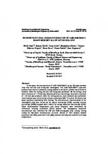
Figure 2: SEM micrographs using secondary electrons showing the Ni-fcc matrix and the secondary phases for the as-welded state - 0h.

3.2. Microstructural SEM analysis and its correlation with ultrasound signal classification The coatings of Inconel 625 alloy deposited by the welding process were submitted to metallographic analysis and SEM, which revealed the Ni-fcc matrix and an extensive amount of secondary phases precipitated (glowing dots) at the intercellular or interdendritic regions. The microstructure of the as-welded alloy condition (0 h) can be seen in Figure 2. The Figure shows an interdendritic secondary phase and some precipitates with cuboidal morphology. The microstructures revealed a Ni-fcc matrix (darkest regions in the image) with some secondary phases precipitated along the intercellular/interdendritic regions (whitest regions in the image). These minor phases were identified as Nb-rich Laves phase and a complex carbide/nitride with cubic morphology. These phases were identified as Nb-rich Laves phase and a complex carbide/nitride with cubic morphology. Figures 3(a), 3(b) and 3(c) show the micrographs of the aged samples for 10, 100 and 200 h, respectively, in which the microstructural modifications 17

(a)

(b)

(c) Figure 3: SEM micrographs using secondary electrons showing the Ni-fcc matrix and the secondary phases of alloy aged at 650°C for 10 (a), 100 (b) and 200 (c) hours.

18

can be seen clearly. Figure 3(a) shows the microstructure corresponding to the sample aged at 650 °C for 10 hours, in which one can see the presence of Laves phase and some cuboidal precipitates of carbides/nitrides. Increasing the time of the thermal exposure to 100 h (Figure 3(b)) there was a significant reduction, i.e., dissolution, in Laves phase content and dimension in the alloy microstructure relatively to the as-welded and 10 h. However, Albuquerque et al. [15] verified that the carbide/nitrides that remained seemed to be unaffected, without any sign of dissolution. As such, quantitatively, there was a larger amount of TiNb carbides/nitrides relative to the Laves phases, which was different to what was seen in the as-welded and 10 h samples [15]. A representative microstructure of the Inconel 625 alloy sample aged at 650 °C for 200 hours is shown in Figure 3(c). In this case, the microstructure indicated an almost complete dissolution of the Laves phases, as the microstructure was now almost totally constituted by the TiNb carbides/nitrides and Ni-fcc matrix. The yet incomplete Laves phase dissolution was evidenced by the residual presence of reminiscent Laves phases [15]. At the thermal aging temperature of 950 °C, a large number of delta phases were observed in samples aged for 10 h. This phase dissolved exponentially with respect to the aging time, as can be seen in Figures 4(a), 4(b) and 4(c) that show the microstructural evolution of the nickel based weld metal, aged 10, 100 and 200 hours at 950 °C, respectively. After being subjected to a thermal aging at 950 °C for 10 hours, the microstructure of the weld metal experienced a significant change. There was a new type of minor phase and the consumption of the prior secondary phase as shown in Figure 4(a). The main change was the formation of a new phase which has a needle-like morphology and is rich in Nb. According the literature, heating Nb bearing nickel alloys to high temperatures, such as 950 °C, may lead to the formation of the Ni3Nb δ-phases with needle-like morphology, which suggested that the new precipitates formed after 10 h at 950 °C were Ni3Nb δ-phases. Carrying on the microstructural study through microscopic analysis, there was a strong reduction in terms of needle-like phases for the Ni-based weld metal after 100 hours of aging. Figure 4(b) shows the microstructures associated to this aging condition and a significant decrease in the amount of the secondary phases can be seen clearly. In addition, many islands with needles-like δ-phases and some cuboidal complex carbides/nitrides rich in Nb and Ti are present. Prolonging the time of exposure to 200 hours (Figure 4(c)) there small precipitates with cubic morphology (carbides/nitrides complex) and a very thin precipitation along 19

(a)

(b)

(c) Figure 4: SEM micrographs using secondary electrons showing the Ni-fcc matrix and the secondary phases of alloy aged at 950°C for 10 (a), 100 (b) and 200 (c) hours.

the grain boundaries in the microstructure, most probably M6C and M23C6 carbides, were found [29, 30]. The literature reports that the δ-phase formation in a significant quantity can be harmful to the mechanical properties due to the precipitation of hardening Ni-based alloys [31]. Therefore, in the case of Inconel 625 alloy, which is a solid-solution strengthened alloy, the precipitation of the δ-phase is only produced after a long exposure time at high temperatures due to the solid solution supersaturated alloy. The precipitation of the δ-phase leads to a decrease in ductility [32]. Another study showed that the hardness and tensile strength decreased with the increase of aging temperature due to the precipitation and coarsening of the delta phase [33].

20

4. Conclusions This work evaluated the efficiency and accuracy of artificial intelligence techniques to classify ultrasound signals, raw data (original) and feature selection methods (preprocessing), background echo and backscattered signals acquired at frequencies of 4 and 5 MHz to characterize, to microstructural characterization the kinetics of phase transformations on a Nb-base alloy, thermally aged at 650 and 950 °C for 10, 100 and 200 hours, as well as in the as-welded condition. In regard to this work, the following conclusions can be pointed out: (1) The results revealed that ultrasonic signal classification using recent artificial intelligence techniques, mainly the OPF, Bayesian and SVM classifiers were sensitive to the microstructural changes in the Inconel 625 alloy, and efficient to identify the formation of the secondary phases during the welding process, as well as the phase transformation kinetics due to the different thermal aging times; (2) The best accuracy rates for thermal aging at 650 °C were obtained using the Bayesian classifier on the backscattered signals acquired with a 4 MHz transducer (93.13%, in 16.43 ms), followed by the OPF with Manhattan distance (91.88%, in 1.40 ms) and the SVM with polynomial kernel (91.88%, in 10,686 ms) classifiers. It is important to point out that the OPF was the fastest classifier in all experiments. For the thermal aging at 950 °C, the best results were obtained using the OPF with Manhattan distance on the background echo signals acquired with the 5 MHz transducer (72.50%, in 0.77 ms), followed by the Bayesian (71.25%, in 258.74 ms) and the SVM with Polynomial kernel (64.38%, in 269,132 ms) classifiers. Here, the OPF was much fast than the others, especially considering the large number of features; (3) The classification using the OPF classifier allows the use of the raw data signals, due to its robustness and fast processing, eliminating the need for preprocessing, and it has a very high classification accuracy. (4) It is very important note that DFA and RS feature extraction methods did not have the expected effect on the OPF results (accuracy, and train and test times), once that its performance was not superior to ultrasonic signals classification using raw data (original) signals. This is because of the robustness of the OPF classifier. However, for others classifiers, the total time was less than the time considering the raw data, and with less accuracy. Based on the results obtained in accurately classifying the ultrasound 21

signals, it is possible to evaluate the aging conditions to which the Inconel 625 alloy was submitted to. With the use artificial intelligence techniques and ultrasound non-destructive inspection, it is possible to predict the best moment to carry out maintenance services, reducing costs and maintenance time. Acknowledgments The first and second author thank National Council for Research and Development (CNPq) and Cearense Foundation for the Support of Scientific and Technological Development (FUNCAP) for providing financial support through a DCR grant #35.0053/2011.1 to UNIFOR. The third author is grateful to CNPq grant #303182/2011-3, and FAPESP grant #2009/162061. All authors are grateful for the support given by the following laboratories of the Federal University of Ceará: Welding Engineering Laboratory (ENGESOLDA), Materials Characterization Laboratory (LACAM), Center of Non-Destructive Testing (CENDE), as well as for the financial support given by the Research and Projects Financing (FINEP), Coordination for the Improvement of People with Higher Education (CAPES) and finally to Petróleo Brasileiro S.A. 5. References [1] M. D. Mathew, K. B. S. Rao, S. L. Mannan, Evaluation of mechanical properties of aged alloy 625 nickel base superalloy using nondestructive ball indentation technique, in: S. Y. Kim (Ed.), Proceedings of 15th International Conference on Structural Mechanics in Reactor Technology (SMiRT-15), Seoul, Korea, 1999. [2] C. Thomas, P. Tait, The performance of alloy 625 in long-term intermediate temperature applications, International Journal of Pressure Vessels and Piping 59 (1994) 41–49. [3] H. K. Kohla, K. Peng, Thermal stability of the superalloys inconel 625 and nimonic 86, Journal of Nuclear Materials 101 (1981) 243–250. [4] O. Boser, The behavior of inconel 625 in a silver environment, Materials Science and Engineering 41 (1979) 59–64. 22

[5] M. J. Cieslak, T. J. Headley, A. D. Romig, The welding metallurgy of Hastelloy alloys c-4, c-22 and c-276, Metallurgical and Materials Transactions A 17A (1986) 2035–2047. [6] M. J. Cieslak, The welding and solidification metallurgy of alloy 625, Welding Journal 70 (1981) 49–56. [7] J. X. Yang, Q. Zheng, X. F. Sun, H. R. Guan, Z. Q. Hu, Formation of phase during thermal exposure and its effect on the properties of k465 superalloy, Scripta Materialia 55 (2006) 331–334. [8] J. N. Dupont, S. W. Banovic, A. R. Marder, Microstructural evolution and weldability of dissimilar welds between a super austenitic stainless steel and nickel-based alloys, Welding Research 82 (2003) 125–156. [9] V. H. C. Albuquerque, P. P. R. Filho, T. S. Cavalcante, J. M. R. S. Tavares, New computational solution to quantify synthetic material porosity from optical microscopic images, Journal of Microscopy 240 (2010) 50–59. [10] V. H. C. Albuquerque, P. C. Cortez, A. R. de Alexandria, J. M. R. S. Tavares, A new solution for automatic microstructures analysis from images based on a backpropagation artificial neural network, Nondestructive Testing and Evaluation 23 (4) (2008) 273–283. [11] V. H. C. Albuquerque, A. R. de Alexandria, P. C. Cortez, J. M. R. S. Tavares, Evaluation of multilayer perceptron and self-organizing map neural network topologies applied on microstructure segmentation from metallographic images, NDT & E International 42 (7) (2009) 644–651. [12] J. P. Papa, R. Y. M. Nakamura, V. H. C. Albuquerque, A. X. Falcão, J. M. R. S. Tavares, Computer techniques towards the automatic characterization of graphite particles in metallographic images of industrial materials, Expert Systems with Applications. 40 (2) (2013) 590–597. [13] V. H. C. Albuquerque, J. M. R. Tavares, P. C. Cortez, Quantification of the microstructures of hypoeutectic white cast iron using mathematical morphology and an artificial neural network, International Journal of Microstructure and Materials Properties 5 (1) (2010) 52–64.

23

[14] J. P. Papa, A. X. Falcão, C. T. N. Suzuki, Supervised pattern classification based on optimum-path forest, International Journal of Imaging Systems and Technology 19 (2) (2009) 120–131. [15] V. H. C. Albuquerque, C. C. Silva, P. G. Normando, E. P. Moura, J. M. R. S. Tavares, Thermal aging effects on the microstructure of Nb-bearing nickel based superalloy weld overlays using ultrasound techniques, Materials & Design 36 (2012) 337–347. [16] V. Shankar, K. B. S. Rao, S. L. Mannan, Microstructural and mechanical properties of inconel 625 superalloy, Journal of Nuclear Materials 288 (2001) 222–232. [17] V. H. C. Albuquerque, E. M. Silva, J. P. Leite, E. P. Moura, V. L. A. Freitas, J. M. R. S. Tavares, Spinodal decomposition mechanism study on the duplex stainless steel UNS S31803 using ultrasonic speed measurements, Materials & Design 31 (2010) 2147–2150. [18] E. M. Silva, V. H. C. Albuquerque, J. P. Leite, A. C. G. Varela, E. P. Moura, J. M. R. S. Tavares, Phase transformations evaluation on a UNS S31803 duplex stainless steel based on nondestructive testing, Materials Science and Engineering: A 516 (2009) 126–130. [19] P. G. Normando, E. P. Moura, J. A. Souza, S. S. M. Tavares, L. R. Padovese, Ultrasound, eddy current and magnetic Barkhausen noise as tools for sigma phase detection on a UNS S31803 duplex stainless steel, Materials Science and Engineering: A 527 (2010) 2886–2891. [20] E. W. Dijkstra, A note on two problems in connexion with graphs, Numerische Mathematik 1 (1959) 269–271. [21] A. X. Falcão, J. Stolfi, R. A. Lotufo, The image foresting transform theory, algorithms, and applications, IEEE Transactions on Pattern Analysis and Machine Intelligence 26 (1) (2004) 19–29. [22] C. Allène, J. Y. Audibert, M. Couprie, J. Cousty, R. Keriven, Some links between min-cuts, optimal spanning forests and watersheds, in: Mathematical Morphology and its Applications to Image and Signal Processing (ISMM’07), MCT/INPE, 2007, pp. 253–264.

24

[23] E. T. Jaynes, Probability Theory: The Logic of Science, Cambridge University Press, 2003. [24] R. O. Duda, P. E. Hart, D. G. Stork, Pattern Classification, WileyInterscience Publication, 2000. [25] B. Schölkopf, A. J. Smola, Learning with Kernels, MIT Press, Cambridge, MA, 2002. [26] V. N. Vapnik, An Overview of Statistical Learning Theory, IEEE Transactions on Neural Networks 10 (5) (1999) 988–999. [27] C. Cortes, V. Vapnik, Support vector networks, Machine Learning 20 (3) (1995) 273–297. [28] J. P. Papa, de V. H. C. Albuquerque, A. Falcão, J. M. R. S. Tavares, Efficient supervised optimum-path forest classification for large datasets, Pattern Recognition 45 (2012) 512–520. [29] C. C. Silva, C. R. M. Afonso, H. C. Miranda, A. J. Ramirez, J. P. Farias, Microstructure of alloy 625 weld overlay, in: AWS Fabtech Conference, Chicago, IL, USA, 2011. [30] C. C. Silva, H. C. Miranda, J. P. Farias, C. R. M. Afonso, A. J. Ramirez, Carbide/nitride complex precipitation- an evaluation by analytical electron microscopy, in: 17th International Microscopy Congress, Rio de Janeiro, Brazil, 2010. [31] D. D. Krueger, The development of direct age 718 for gas turbine engine disk applications, Vol. 20 of Superalloy 718 – Metallurgy and Applications, The Minerals, Metals and Materials Society, 1989. [32] V. Shankar, M. Valsan, K. B. S. Rao, S. L. Mannan, Room temperature tensile behavior of service exposed and thermally aged service exposed alloy 625, Scripta Materialia 44 (2001) 2703–2711. [33] M. D. Mathew, K. B. S. Rao, S. L. Mannan, Creep properties of serviceexposed alloy 625 after re-solution annealing treatment, Materials Science and Engineering A 372 (2004) 327–333.

25