AUTOMATIC RAILWAY CLASSIFICATION USING SURFACE AND SUBSURFACE MEASUREMENTS George Kantor*, Herman Herman*, Sanjiv Singh*, John Tabacchi†, and William Kaufman† *The Robotics Institute, Carnegie Mellon University, Pittsburgh, PA, 15213 USA Applied Adanvced Technologies, Carnegie Mellon Research Institute, Pittsburgh, PA, 15230 USA Phone Int +(412)268-4749, Fax Int +(412)268-5895, E-mail:
[email protected]
†
Abstract: The proper assessment of railroad condition requires the consideration of a number of factors. Some factors, such as the condition of the ties, can be measured by inspecting features visible from the surface of the railway. Other factors, such as the condition of the ballast, require subsurface measurements. Extensive human resources are currently applied to the problem of evaluating railroad health. Here we present the results of a study in automatic railroad classification that combines surface and subsurface measurements to characterize the railroad condition. To obtain surface measurements, we generate a 3-D profile of the railroad surface with a vision system that employs a laser light stripe. Subsurface measurements were made using ground penetrating radar (GPR). Principal component analysis was used to reduce the dimension of the raw data. Classifiers were trained on the resulting data using both memory based and Bayesian methods. The results are presented. Keywords: pattern recognition, classification, railroad, ground penetrating radar
1 INTRODUCTION
2 PRIOR WORK
The railroad network must be continuously maintained to assure the safe and timely delivery of freight and passengers. This maintenance effort is complicated by the fact that accurate assessments of track condition are difficult and expensive to obtain. In many cases, efficient data collection tools exist, but human experts are required to analyze the data and identify sections of track that require maintenance. With thousands of miles of track, this is often impractical. In this paper, we apply pattern recognition techniques in order to automate the analysis of railroad data. In order to generate a comprehensive picture of railroad health, we combine surface and subsurface data. A laser light striping system is used to measure and assess tie surfaces for cross tie classification. Ground penetrating radar (GPR) is used to detect subsurface anomalies in the ballast, or substructure. Taken together, the surface and subsurface classifiers provide an important step towards the automated, comprehensive assessment of railroad maintenance requirements. The classification techniques used here rely on principal component analysis, memory based learning, and Bayesian pattern recognition. These techniques have been established as powerful tools in a number of domains including face identification, sonar data analysis, and speech recognition. The work presented here represents a novel application of these techniques to the problem of railroad condition assessment.
A considerable body of work has been published on the problem of applying recent technology advances to aid in the classification and management of railroad systems. Computers have been used to help automate the collection and analysis of railroad data as early as 1967 [Railway and Track Structures, 1971]. Sensing systems capable of collecting various track geometry data have been developed and applied. Systems capable of recording track geometry and strength have been developed for railroad cars [Ebersohn and Selig, 1994] and high-rail vehicles [Zarembski and McCarthy, 1995]. Computer vision systems have been applied to monitor rail wear [Magnus, 1995], measure rail width [Ryabichenko et al, 1999], and produce a database of continually scanned visual images [Sasama, 1994]. These systems facilitate the automated collection of large amounts of railroad data. However, the data must be parsed and analyzed by a human expert before it can be used to make maintenance decisions. Similar advances have been made in the measurement of ballast and subgrade condition. The primary tool for non-destructive measurement of subsurface condition is ground penetrating radar (GPR). GPR has been used to identify fouled ballast and trapped water on an experimental railroad test bed [Gallagher et al, 2000]. In [Sussmann et al, 1999] GPR was found to be particularly useful for locating drainage problems and identifying areas of similar substructure condition. Other efforts have successfully combined GPR with infrared imaging systems to detect subsurface defects in railroad track beds
[Weil, 1995]. While these results are promising, GPR data must currently be analyzed by human experts. The large amount of time and human resources required make GPR too expensive for common use. There is an extensive body of work which addresses the problem of automated analysis, pattern recognition, and classification of sensor data. We use a small subset of this work here. Our use of principal component analysis (PCA) to reduce data dimension is borrowed directly from computer vision efforts to automatically recognize faces [Sirovich and Kirby, 1987; Turk and Pentland, 1991] and three dimensional objects [Nayar et al, 1996]. We also rely on results of previous researchers to classify the resulting reduced-dimension data. Once such technique is memory based learning, in which data is efficiently stored using kd-trees and classification is achieved using local regression models [Schneider and Moore, 2000]. Another useful classification technique employs Bayes’ formula to identify the most likely class associated with a given data vector [Ahlea, 1996].
3 CLASSIFICATION METHODS The goal of this study is to automatically determine railroad class (eg. “good” or “bad”) from sensor data. This problem is known as classification. A classifier takes a data point (or “query point”) as its input and returns as an output an estimate of the class associated with the data point. Both of the classification methods addressed in this paper require training. They “learn” from a set of data that has been classified using some other method, such as evaluation by a human. For this, a large number of data points must be collected and each data point must be assigned a class or label. The data set, which consists of the data points together with their labels, is then divided into a training set and a test set. As their names imply, the training set is used to train the classifier and the test set is used to evaluate the results. The general idea of training is that training set data points are presented to the classifier, which adjusts its internal parameters to minimize some measure of the error between the estimated class and the actual label. The details vary from method to method and are described below.
3.1 Memory Based Classification In memory based classification, every data vector and associated label from the training set is stored in computer memory. A query point is then classified by finding a set of training points in the neighborhood of the query point, fitting the neighboring points and their labels to some model, and using this model to estimate the class. To implement this, we used a locally weighted learning
package named Vizier 1.0 [Schneider and Moore, 2000]. Vizier performs two main functions that make memory based classification possible. First, it employs a data structure called a kd-tree in order to efficiently organize and retrieve data the training set data. This is necessary to find, in a timely manner, training set data points which are close to a given query point. Vizier can then perform its second function, which is to create a model using locally weighted linear regression and use the model to estimate the class of the query point.
3.2 Bayesian Classification If the distributions of the data points within the possible classes are Gaussian, then Bayes' formula can be used to determine the most likely class associated with a given data point. Bayes’ formula gives p( x | wi )p( wi ) p( wi | x) = (1) p( x ) as the probability that the class wi is correct given the data vector x. The Gaussian assumption means that (x − mi )T Ci−1 (x − mi ) exp 2 (2) p( x | wi ) = n (2π ) det(Ci ) where mi is the mean and Ci is the covariance matrix associated with the ith class. For a given x, it can be shown [Ahlea, 1996] that the class that maximizes the conditional probability in Equation (1) is the same class that minimizes the expression 1 d i ( x) = log(det (Ci )) − log( p( wi ) ) 2
+
(x − mi )T Ci−1 (x − mi ) . 2
(3)
The quantity d i is known as the Bayesian metric from mi to x. The “training” of a Bayesian classifier consists of using training set data to estimate the mean, covariance matrix, and prior probability p( wi ) for each possible class. Once these parameters are known, a query point x can be classified by evaluating Equation (3) for each i and choosing the class wi associated with the smallest value. 3.3
Discussion
The primary advantage of memory based classification is its flexibility and generality. The memory based method does not assume anything about the distribution of the data, and the decision surfaces that result can take any shape. This contrasts with the Bayesian method, which assumes the data has a Gaussian distribution. This means
that the resulting decision surfaces must be quadratic. As a result, we expect memory based classification to provide more accurate results, especially when the Gaussian assumption does not hold. The main disadvantage of memory based classification is that it is memory intensive. This especially becomes a problem as the input dimension and number of training points get large. The time required to retrieve the appropriate data points can be prohibitive in these cases. The Bayesian classifier does not have this problem. All of the necessary information from the training set is stored in the mean vectors and covariance matrices for each class. The Bayesian method is also computationally simpler, especially when the dimension of the data is high. These two factors combine to make a Bayesian classifier easier to implement than its memory based equivalent.
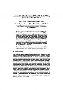
4 SENSOR OPERATION In this section we briefly describe the physical principles of operation of the sensing technologies used in this study. We use GPR to measure subsurface characteristics of the railroad bed and we use laser light striping to measure surface parameters. A modified railroad push-cart borrowed from Allegheny Valley Railroad was used as a data collection platform for both the surface (laser light stripe system) and subsurface (GPR) sensors. The cart was equipped with a small generator to provide electrical power to both systems. A diagram of the cart set-up is shown on the left side of Figure 1. Details regarding the GPR and light stripe set-up are contained in the following discussions.
4.1 Ground Penetrating Radar A brief description of GPR principles of operation is contained here. For a more detailed description the reader is referred to [Herman, 1997]. The GPR antenna sits on the surface of the ground and emits an electromagnetic pulse downward into the soil. As the pulse travels through the soil, its energy is refracted and partially reflected whenever it encounters a discontinuity in the electrical properties of the soil. The reflected energy travels back towards the surface where it is measured by the antenna. If the speed of the pulse is known, then the distance between the discontinuity and the antenna can be determined. The magnitude of the discontinuity is contained in the strength of the reflection. Discontinuities detected by GPR result from underground features such as objects, voids, water, and soil layer interfaces.
Figure 1. A sample GPR return. The vertical axis represents depth into the ground. Each column of pixels represents a single GPR scan, so plotting multiple successive scans provides an “image” of subsurface features. In a typical application, the GPR antenna is moved along the ground in a straight line at a constant speed while sending and receiving pulses at a constant rate. The result is a collection of evenly spaced GPR returns. This collection can be displayed graphically as shown in Figure 1. The vertical axis represents distance into the ground where the surface is located at the top of the figure and the maximum depth measured by the system is at the bottom. Each column of pixels represents a single GPR scan, and the leftmost column corresponds to the first scan. The horizontal scale depends on the speed and pulse rate of the GPR. For example, if the antenna was moving at a speed of 1 meter/second while reading 10 scans per second, each scan (and hence each column of pixels in Figure 2) would be 0.1 meters apart. The GPR unit we chose to use was an SIR-2000 manufactured by Geophysical Survey Systems, Inc. The unit was used with a 1 GHz dipole antenna. The antenna was mounted on a flexible polymer sheet that slid along the ground in front of the cart.
4.2 Laser Light Striping Laser light striping is a vision-based technique of generating a 3-D profile of visual scene. A line of laser light is projected onto the surface being profiled while a camera records the resulting image. The known geometry of the camera and the light stripe can then be used to triangulate the 3-D locations of the points on the surface that are illuminated by the laser.
Figure 2. This figure shows the data collection set-up and illustrates the laser light stripe preprocessing. The two diagrams on the left of the figure depict how the laser light stripe system and GPR antenna are mounted to the test cart. The figure in the middle is a sample image taken from the light stripe system’s camera. The plot on the right contains the data vector extracted from the sample image. A depiction of light striping set-up and operation is shown in Figure 2. Both light striper and camera were mounted to a cart. The camera was positioned to look straight down at the track with its field of view extending from about the middle of the tie to the rail. The light striper was mounted at an angle so that it projected its line into the field of view of the camera. The light striper was oriented so that, for flat, level ground, the projected stripe would be a line parallel to the ties.
5 SUBSURFACE MEASUREMENTS In this section we describe the procedures, algorithms, and results for automated subsurface analysis using GPR.
5.1 Data Collection The GPR unit was set to a depth of approximately 1 meter. The depth resolution was set to 510 samples per scan, which corresponds to a spatial resolution of 2mm. During data collection, the data cart was moved along the track at a uniform velocity of 1 meter per second. With a scan rate of 32 scans per second, this corresponds to a spatial scanning resolution of about 3 cm. We collected data from two non-adjacent “good” sections (denoted G1 and G2) and two nonadjacent “bad” sections (denoted B1 and B2). Data from sections G1, G2, B1, and B2 was taken in adjacent 10 meter segments. A total of 8 segments were collected from G1, these segments were labeled G11 through G18. Likewise, 5 segments were taken from G2, 4 from B1, and 2 from B2. Upon visual inspection of the GPR data, it was found that the second and fifth segments from G1 and the second segment from G2 contained strong reflections indicating the presence of some
unknown subsurface anomaly. These segments were relabeled as U12, U15, and U22. The data collected from G1, B1, and U1 formed a training set with approximately 24,000 data points. G2, B2, and U2 formed the 14,000 point test set.
5.2 Preprocessing The collected data segments were preprocessed in order to facilitate classification. First, the data were filtered horizontally to remove small disturbances as well as fluctuations due to the ties. The filter used was a simple moving average with a window size of about 2 meters. Next, the surface reflection was removed by eliminating the top 100 samples from each scan. We also removed the bottom 100 samples from each because the GPR readout contained excessive noise in this region. Finally, the DC bias of each segment was removed by subtracting the average return over the training set at each depth. For both memory based and Bayesian classifiers, PCA was used to reduce the dimensionality of the data set. In keeping with the separation between test data and classifier training, the PCA transform was found using only the training data. Figure 3 illustrates the effect of the PCA transform on a subset of the test data. PCA effectively reduced the dimension of the data set from 300 to 5.
5.3 Results Memory based and Bayesian classifiers were trained using the preprocessed GPR data. The results are shown in Table 1. The first column gives the overall performance, i.e. the percentage of correctly classified data points over the whole test set. The next three columns give the accuracy within each class.
Figure 3. This figure depicts the effect of principal component analysis on some example data. The images on the left show samples of GPR data that has been horizontally filtered, windowed, and removed of DC bias. The images on the right show the 20 most significant components of the same data sets after PCA transform. The components are plotted in order of significance from top to bottom. Note that almost all of the information is contained in the top few rows. In this example, we were able to reduce the dimension of the data set from 300 to 5. The memory based method is more accurate than the Bayesian method, especially in discriminating between “good” and “unknown”. This is because the distribution of points in the “unknown” class is not well modeled as Gaussian. Still, the Bayesian method works reasonably well, and it is so simple to implement that it is worth consideration. Table 1. Classification results for GPR data. overall
good
bad
unknown
memory
96.4%
95.8%
99.5%
84.0%
Bayesian
93.3%
92.4%
98.4%
71.9%
6 SURFACE MEASUREMENTS In this section we describe the procedures, algorithms, and results for automated cross tie analysis using laser light striping. With the ability to extract 3-D information about the surface of a tie, the light striper should be able to detect the presence of cracks and warping in ties.
6.1 Data Collection We recorded light stripe images of a number of ties for the purpose of training and testing a classifier. The images were collected using the experimental set-up described in Section 4. Data was obtained for a total of 513 ties, with a minimum of 6 images recorded for each tie. The resulting
images were “good” or “bad” according to a visual inspection of the associated ties. Of the 513 ties, 295 were labeled “good” and the remaining 218 were labeled “bad”. The data was then separated into training and test sets.
6.2 Preprocessing The main preprocessing step for the light striping system is to extract the horizontal position of the stripe for each row of pixels in the image. The ith element of the resulting data vector contains the location, in pixels, of the pixel where the light stripe intersects the ith row. If it is not possible to locate the light stripe in a given row, the corresponding element of the data vector is set to 0. The result of this extraction procedure is depicted in the right side of Figure 1. For classification purposes, we only considered the portion of the stripe which is projected onto the ties. Recall that multiple images were recorded for each tie. To obtain a single vector for a given tie we simply took the average of all of the data vectors associated with that tie. PCA was then applied to reduce the dimension. For the collected data set, PCA successfully reduced the dimension from 125 to 2.
6.3 Results Memory based and Bayesian classifiers were trained using the preprocessed light stripe data. The results are shown in Table 2. This table should be interpreted in similarly to Table 1. Both classifiers work very well, with the memory based method slightly outperforming the Bayesian classifier.
Table 2. Classification results for light stripe data. overall
good
bad
memory
97.1%
98.4%
95.5%
Bayesian
96.2%
97.7%
94.4%
7 CONCLUSION Pattern recognition techniques show promise as tools in automated railroad inspection. In this study, we have developed classifiers capable of distinguishing between good and bad ballast using GPR data. We have also developed a classifier that employs laser light striping to evaluate tie health. In both cases, the combination of a PCA dimension reduction step with memory based classification methods provides an accurate classifier with a reasonable amount of computational overhead. The generality of the results here is inherently restricted by limitations of our data set. This is particularly true for the GPR studies, where the amount of data collected was small, the data was not very diverse (i.e. there were only three classes of data), and the labeling was unreliable. Future work in this regard is to train and test a new classifier on better data set. Additional work on the sensor fusion aspect of the problem is also required. Initial efforts should futher address the merging of light stripe and GPR data. The light stripe system should provide some information about ballast health by detecting vegetation and profiling the surface of the ballast. Other data sources should also be considered for fusion. Likely candidates include infrared imaging, ultrasonic, and geometry car measurements.
REFERENCES [Ahlea, 1996] Ahlea Systems Corp., Pattern Recognition Toolbox for use with MATLAB, User’s Guide, 1996. [Ebersohn and Selig, 1994] W. Ebersohn and E.T. Selig, Use of geometry measurements for maintenance planning, Transportation Research Record No. 1470, Railroad Research Issues, pages 84-92, 1994. [Gallagher et al, 2000] G. Gallagher and Q. Leiper and M. Clark and M. Forde, Ballast evaluation using ground penetrating radar, Railway Gazette International, pages 101-102, February 2000. [Herman, 1997] H. Herman, Robotic Subsurface Mapping Using Ground Penetrating Radar, PhD thesis, Carnegie Mellon University, May 1997.
[Magnus, 1995] D.L. Magnus, Non-contact technology for track speed rail measurements (ORIAN), in Proceedings of the SPIE, Nondestructive Evaluatoin of Aging Railroads, 2458:45-51, 1995. [Nayar et al, 1996] S.K. Nayar, S.A. Nene, and H. Murase, Real-time 100 object recognition system, in Proceedings of the 1996 IEEE International Conference on Robotics and Automation, pages 2321-2325, April 1996. [Ryabichenko et al, 1999] R.B. Ryabichenko, S.B. Popov, and O.S. Smoleva, CCD photonic systems for rail width measurement, in Proceedings of the SPIE, Photonics for Transportation, 3901:37-44, 1999. [Sasama, 1994] H. Sasama, Maintenance of railway facilities by continuously scanned image inspection, Japanese Railway Engineering, 27:1-5, January 1994. [Schneider and Moore, 2000] J. Schneider and A. Moore, A locally weighted learning tutorial using Vizier 1.0, Technical Report CMU-RITR-00-18, The Robotics Institute, Carnegie Mellon University, 2000. [Sirovich and Kirby, 1987] L. Sirovich and M. Kirby, Low dimensional procedure for the characterization of human faces, Journal of Optical Society of America, 4(3):519-524, 1987. [Sussmann et al, 1999] T.R. Sussmann, F.J. Heyns, and E.T. Selig, Characterization of track substructure performance, in Recent Advances in the Characterization of Pavement Geomaterials, Geotechnical Special Publication, American Society of Civil Engineers, pages 37-48, 1999. [Turk and Pentland, 1991] M.A. Turk and A.P. Pentland, Face recognition using eigenfaces, in Proceedings of the IEEE Conference on Computer Vision and Pattern Recognition, pages 586-591, 1991. [Railway and Track Structures, 1971] Mechanized, automated, computerized, Railway and Track Structures, pages 18-21, March 1971. [Weil, 1995] G.J. Weil, Non-destructive, remote sensing technologies for locating subsurface anomalies on railroad track beds, in Proceedings of the SPIE, Nondestructive Evaluation of Aging Railroads, 2458:74-81, 1995. [Zarembski and McCarthy, 1995] A.M. Zarembski and W.T. McCarthy, Development of nonconventional tie and track structure inspection systems, Transportation Research Record No. 1489, Railroad Transportation Research, pages 26-32, 1995.