REGARDS ON TWO REGARDS BY MESSIAEN: AUTOMATIC SEGMENTATION USING THE SPIRAL ARRAY Elaine Chew University of Southern California Viterbi School of Engineering Epstein Department of Industrial and Systems Engineering Integrated Media Systems Center
[email protected] ABSTRACT Segmentation by pitch context is a fundamental process in music cognition, and applies to both tonal and atonal music. This paper introduces a real-time, O(n), algorithm for segmenting music automatically by pitch collection using the Spiral Array model. The segmentation algorithm is applied to Olivier Messiaen’s Regard de la Vierge (Regard IV) and Regard des prophètes, des bergers et des Mages (Regard XVI) from his Vingt Regards sur l’Enfant Jésus. The algorithm uses backward and forward windows at each point in time to capture local pitch context in the recent past and not-too-distant future. The content of each window is mapped to a spatial point, called the center of effect (c.e.), in the interior of the Spiral Array. The distance in the Spiral Array space between the c.e.’s of each pair of forward and backward windows measures the difference in pitch context between the future and past segments at each point in time. Segmentation boundaries then correspond to peaks in these distance values. This paper explores and analyzes the algorithm’s segmentation of post-tonal music, namely, Messiaen’s two Regards, using various window sizes. The computational results are compared to manual segmentations of the pieces. Taking into account the entire piece, the best case computed boundaries are, on average, within 0.94% (for Regard IV) and 0.11% (for Regard XVI) of their targets. 1.
INTRODUCTION
Segmentation by context is a necessary part of music processing both by humans and by machines. Efficient and accurate algorithms for performing this task are critical to computer analysis of music, to the analysis and rendering of musical performances, and to the indexing and retrieval of music using largescale datasets. Computational modeling of the segmentation process can also lead to insights on human cognition of music. This paper will focus on the problem of determining boundaries that segment a piece of music into contextually similar sections according to pitch content. In particular, the algorithm will be applied to Olivier Messiaen’s (1908-1992) Regard de la Vierge and Regard des prophètes, des bergers et des Mages, the fourth and sixteenth pieces in his Vingt Regards sur l’Enfant Jésus (1944). The O(n) segmentation method uses the Spiral Array model [1], a mathematical model that arranges musical objects in three-dimensional space so that inter-object distances mirror their perceived closeness. The Spiral Array represents tonal objects at all hierarchical levels in
the same space and uses spatial points in the model’s interior to summarize and represent segments of music. The array of pitch representations in the Spiral Array is akin to Longuet-Higgins’ Harmonic Network [7] and the tonnetz of neo-Riemannian music theory [4]. The key spirals, generated by mathematical aggregation, correspond in structure to Krumhansl’s network of key relations [5] and key representations in Lerdahl’s tonal pitch space [6], each modeled using entirely different approaches. The present segmentation algorithm, named Argus, is the latest in a series of computational analysis techniques utilizing the Spiral Array. The Spiral Array model has been used in the design of algorithms for key-finding [2] and off-line determining of key boundaries [3], among other things. The previous model for determining key boundaries is the one most relevant to this paper. This earlier algorithm requires knowledge of the entire piece and the total number of segments, and does not compute in real-time. So far, the Spiral Array has only been used in the analysis of tonal music. This paper extends the Spiral Array model’s applications to real-time segmentation and to the analysis of post-tonal music. The Argus algorithm for automatic segmentation uses only the outermost pitch spiral in the Spiral Array model and the interior space to compute a distance between the local context (captured by a pair of sliding windows) immediately before and after each point in time. The distance measure peaks at a segmentation boundary and the peaks can be used to identify such boundaries in realtime. Since the segmentation algorithm detects boundaries between sections employing distinct pitch collections, the procedure does not depend on key context and can be applied in general to both tonal and atonal music. The method is highly efficient, computing in O(n) time, and requires only one left-toright scan of the piece. The algorithm is tested on Messiaen’s Regards IV and XVI and the results presented for various window sizes. The computational results are compared to manual segmentations of the piece. Related work on finding local tonal context include Temperley’s dynamic programming approach to determining local key context [10], Shmulevich & YliHarja’s median filter approach to local key-finding [9] and Toiviainen & Krumhansl’s self-organizing map approach to determining and visualizing varying key strengths over time [11]. The focus of these methods are on determining the local key context rather than finding the segmentation boundaries. The methods center around key-finding, which applies only to tonal music.
(c) major key representations
(b) major triad representations
(a) pitch representations
Figure 1. The Spiral Array model.
The remainder of the paper presents a concise overview of the Spiral Array model followed by a description of the segmentation algorithm. Then, in Section 3, a descriptive analysis of Regard IV is followed by a detailed analysis of the computational results and comparisons between the computed and manually assigned boundaries. A similar treatment of Regard XVI is presented in Section 4, followed by discussion and conclusions in Section 5. 2.
CM(k) = w1P(k) + w2P(k+1) + w3P(k+4),
THE SPIRAL ARRAY MODEL
where w1 ≥ w 2 ≥ w 3 > 0 and
This section provides an overview of the structure of, and underlying concept (namely, the center of effect) behind, the Spiral Array model [1]. The description of the proposed segmentation algorithm follows the introduction to the Spiral Array. 2.1. The Model’s Structure The Spiral Array model represents pitches on a spiral so that spatially close pitch representations form familiar higher-level tonal structures such as triads and keys. The model represents each higher-level object as the convex combinations of its lower-level components. These weighted sums of representations of the components result in spatial points in the interior of the pitch spiral. For example, Figure 1 shows the hierarchical construction of major key representations, from pitches to triads to keys. Figure 1(a) shows the pitch spiral – adjacent pitches along the spiral are related by intervals of a Perfect Fifth; each turn of the spiral contains four pitch representations, as a result, vertical neighbors are a Major Third apart. Pitch representations can be generated by the following equation: È r sin kp 2 ˘ Í ˙ P(k) = Í r cos kp 2 ˙ Í ˙ kh ÍÎ ˙˚
( (
) )
indexed by its number of Perfect Fifths from a reference pitch. The model assumes octave equivalence so that all pitches with the same letter name map to the same spatial point. Pitches that define a triad form compact clusters. They also form the vertices of a triangle. Each triad is represented by the convex combination of its component pitches, that is to say, a point in the interior of the triangle. For example, the major triad is defined as:
(1)
where r is the radius of the spiral and h is the vertical ascent per quarter turn. Each pitch representation is †
Â
3 w i=1 i
(2)
= 1.
The sequence of major triad representations also forms a spiral, as shown by the inner spiral in Figure 1(b). Three adjacent major triads uniquely define the pitch collection for a major † key. They also form the IV, I and V chords of the key. Hence, major keys are defined as: T M(k) = w 1C(k) + w2C(k+1) + w3C(k–1), where w1 ≥ w 2 ≥ w 3 > 0 and
Â
3 w = i=1 i
(3)
1.
Again, the sequence of major key representations form a spiral. This major key spiral is shown as the innermost spiral in the illustration in Figure 1(c). Corresponding definitions exist for† the minor triad and key representations. The Spiral Array model is calibrated using mathematical constraints to reflect perceived closeness among the different entities. For example, in the definition of the major triad, the weights are constrained so that the weight on the root is no less than the weight on the fifth, which is no less than the weight on the third. Since the segmentation algorithm uses only the pitch representations, we shall concern ourselves only with parameter selection for the pitch spiral, namely, the choice of r and h. The pitch spiral is uniquely defined by its aspect ratio h/r. The goal is to constrain the parameters so that the distance between any two pitch representations correspond to their perceived closeness. Suppose the desired rank order of the interval distances is as follows: {(P5/P4), (M3/m6), (m3/M6), (M2/m7), (m2/M7), (d5/A4)}, where P denotes a perfect interval, M a major
interval, m a minor interval, d a diminished interval and A an augmented interval. Algebraic manipulation shows that the mathematical constraints on the aspect ratio, √(2/15) £ h/r £ √(2/7), produce the desired ranking of interval relations. In the remainder of the paper, h/r is always set to √(2/15), the case where major triad pitches form equilateral triangles. 2.2. The Center of Effect One of the main ideas behind the Spiral Array model is the use of points in the interior of the spiral to represent collections of pitches. More specifically, any pitch collection can generate a center of effect (c.e.), a weighted sum of the pitch representations that is a point in the model’s interior. This concept was demonstrated in the definition of the major triad and major key in the previous section. Generalizing the idea, any segment of music can also generate a center of effect. In previous algorithms for tonal induction and segmentation [2][3], the c.e. of choice was one in which each pitch position was weighted by that pitch’s proportional duration in the segment of music. The current implementation of the segmentation algorithm uses a slightly different c.e., one that measures the salience (weight) of the pitch not just by its duration, but also by the number of other pitches present at the same time. At each slice of time containing pitches of uniform duration, the average of the represented pitch positions is calculated, thus generating a c.e. for that time slice. The average of all the c.e.’s of all time slices within the given window is the c.e. for the chosen segment of music. Suppose n j is the number of active pitches in the j-th time slice, and p i,j is the Spiral Array position of the i-th pitch in the j-th time period, then the formal definition of the c.e. of the musical segment in the time interval [a,b] is:
c a ,b =
1 b - a +1
b
nj
ÂÂ j = a i =1
p i, j nj
(4)
In this definition of the c.e., all else being equal, a note of longer duration would receive a weight greater than one accorded a note of shorter duration; and, a note that sounds singly would receive a greater weight than one that sounds simultaneously with other pitches as part of a chord. Other definitions can be devised to emphasize the metric weight of the note. This duration- and independence-based definition is the one used in the current implementation of the segmentation algorithm. This is not an unreasonable choice in the case of Messiaen’s music, given the frequent metric changes in his Vingt Regards.
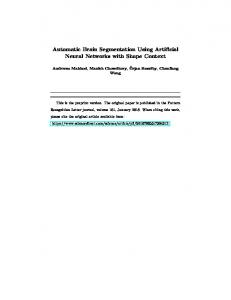
Figure 2. Idea behind the segmentation algorithm.
2.3. The Argus Segmentation Algorithm The intuition behind the segmentation algorithm is that at a boundary point, the distance between the c.e.’s of the local section immediate preceding and succeeding the boundary is at a maximum. This idea is illustrated in Figure 2. Suppose the piece consists of three sections,
(a) before the first boundary
(d) maximum at second boundary
(b) maximum at first boundary
(e) beyond the second boundary
(c) between the first and second boundaries
(f) the end
Figure 3. Progression of segmentation algorithm.
Figure 5. Manual segmentation of Messiaen’s Regard IV into component sections.
that employ distinct pitch sets, with boundaries at B1 and B2 (B0 and B3 represent the beginning and end of the piece) as shown in Figure 2. At B 1, the distance between the c.e.’s of the preceding light gray section and the succeeding dark gray section (represented by discs of the corresponding colors) is maximized. Sliding the double window across the entire piece produces a plot of d over time that contains local maxima at the boundaries as depicted schematically in Figure 3, where the scissors indicate the actual boundaries of the piece. As can be seen in the diagram, the algorithm requires only one left-to-right scan of the piece and computes in O(n) time.
the score tempo changes at the beginning of each section. A
Section A: asymmetric 6+7 motif
B
2.4. When to Take a Peak Seriously? There exist many local maxima in the graph of d over time. One question remains: how can one separate the significant peaks from the insignificant ones? One objective measure is to only select maxima that are above a given threshold, say, one standard deviation, sd, from the mean d value, md. If the distances can be approximated by a normal distribution, values more than two standard deviations above the mean have a statistical significance of approximately 97.5%. For a real-time realization of the algorithm, this threshold needs to be pre-determined. For the purposes of evaluating the algorithm in this paper, the threshold is assigned after computing all the distances. 3.
MESSIAEN’S REGARD IV
We first apply the segmentation algorithm described in the earlier part of this paper to Regard de la Vierge, the fourth piece in Olivier Messian’s (1908-1992) Vingt Regards sur l’Enfant Jésus (1944). Any discussion of the computational results first requires some ground truth to which to compare the algorithm’s outcomes. In Section 3.1, a manual analysis of the piece is presented, showing the different sections. Then, the computational results using various forward and backward window sizes are compared to this manual segmentation in Section 3.2.
Section B: fluid triplet motif and 6-chord sequence
C
Section C: rhythmic motif and stacked octaves Figure 4. Sections in the fourth Regard and their defining motifs.
The sequence of sections in the piece, ABACABAC, can be visualized using the bar in Figure 5. The numbers at the boundaries correspond to the number of sixteenth notes from the beginning of the piece. In this particular counting scheme, the sixteenth notes in the triplet motif in Section B are counted as full-valued sixteenth notes and all ornaments are grouped with the pitch set which they embellish. (a) combination of motivic material in A sections in second half of piece.
3.1. Manual Segmentation of Regard de la Vierge A manual analysis of Messiaen’s Regard de la Vierge yields three main sections with defining motifs as shown in Figure 4. The first, call it Section A, presents phrases built on an asymmetric 6+7 motif shown in Figure 4. Section B contains the fluid triplet motif and a second more angular and wide-ranging six-chord sequence. Section C is the most energetic of the three and contains a rhythmic motif whose baseline turns into a second motif with stacked octaves. The square patches on the left show the grayscale tone used to represent that section. The demarcation between sections is clear from the score. In addition to the different motivic material, the composer also writes into
(b) retrograde motif i n return of Section B.
Figure 6. Variations in the return of the sections.
Some variations occur in the return of each section in the second half of the piece. For example, the A sections in the second half of the piece combine material
from Section A (main motif) and Section C (baseline of first motif) – see Figure 6(a). In the return of Section B, the triplet motif is reversed as shown in Figure 6(b). However, the note material is still primarily the same in each case, and the sections are recognizable as being similar to their earlier counterparts. 3.2. Automatic Segmentation Messiaen’s Regard de la Vierge was encoded in text format so that at each sixteenth note instance, the names of all pitches present is known. As in the previous section, the sixteenth notes in the triplet figure in Section B’s first motif are assumed to be full-valued sixteenth notes in this encoding and all ornaments are grouped with the notes that they embellish. Note that an encoding that respects the tempo changes (one that would be closer to the performed timing) would be slightly different but produce similar results. The segmentation algorithm was implemented in Java. Recall that the algorithm requires the user to specify the forward and back window sizes shown in Figure 7. In this paper, we consider the algorithm’s results when f = b = 60, 40, 20 and 10.
Figure 7. Parameters in the algorithm: the forward and backward window sizes, f and b.
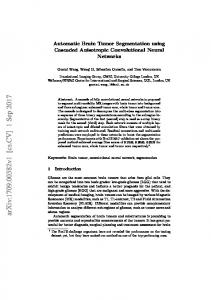
3.3. Results when f = b = 60 The segmentation boundaries are computed with forward and backward windows of size 60 (sixteenth notes). The resulting distance values are plotted over time and shown in Figure 8. The horizontal solid line cutting crossing the plot of d marks the average d value, md. The dotted lines correspond to one and two standard deviations above the mean, md, + sd and md + 2sd, respectively. Maxima above one standard deviation are marked by vertical lines in the plot. Overlaid on the top part of the chart is the manual segmentation of the piece for comparison with the computed segmentation boundaries. The average absolute discrepancy between the computed and actual boundaries is 8.43 sixteenth notes. Comparing this number with the number of sixteenth notes (893 in total), the boundaries are, on average, off by 0.94%. Most of the discrepancies are caused by bridge material that either contains pitch collections of the upcoming sections or motivic material borrowed from other sections. Two examples are given in Figure 9, where the outlined arrows indicate the computed boundaries and the solid arrows indicate the actual boundaries. Figure 9(a) explains the discrepancy between the computed boundary at 196 and the actual boundary at 208. In this case, the final chords in Section B are re-spelt enharmonically (with sharps instead of flats) to prepare for the return of Section A. Figure 9(b) explains the largest discrepancy value (corresponding to the peak at 719), which occurs where the Section C motif is appended to the end of Section B before the return of Section A.
Figure 8. Plot of d over time (in sixteenth notes), f = b = 60 [ md = 0.7418, sd = 0.5083 ]. Section C motif
(a) enharmonic spelling of chord pitches pitches in B in preparation for return of A
(b) largest discrepancy caused by motivic material from Section C appended to the end of Section B before the return of Section A.
Figure 9. Analysis of difference between computed and actual boundaries (
computed,
actual).
Figure 10. Plot of d over time, f = b = 40 [ md = 0.6821, sd = 0.5343 ].
3.4. Results when f = b = 40 Next, the algorithm is applied with forward and backward context windows that are 40 sixteenth notes wide. The results are documented in Figure 10. At f = b = 40, the plot of d over time shows some ambiguity in determining the significant peaks. The three peaks inside Section C at times 385, 423 and 451 are higher than the one for the boundary at 662. In Section C, 385 and 451 correspond approximately to the beginning to the octave motif subsections (at 386 and 448); and, 423 corresponds to another smaller boundary between subsections. Note that the similarity between the ABA sections in the first and second half of the piece are now more apparent. 3.5. Results when f = b = 20 When the window sizes are reduced to 20 sixteenth notes, the peaks at the section boundaries still exist, however, the peaks representing the local boundaries within Section C have become more pronounced (see Figure 11). In the first Section C, the highest peaks (at 385 and 447) mark the beginnings of the octave motif (exact positions in the score are at 386 and 448). The beginning of the second motif in Section B is marked by a peak at 173 and a corresponding but smaller peak
can be seen at 699. In addition to the more pronounced similarity between the two ABA sections, the repeated patterns in the more homogenous Section A are now visible as sequences of low-lying humps. 3.6. Results when f = b = 10 When the window sizes are reduced to 10 sixteenth notes, the local peaks within the large sections (especially C) dominate the picture (see Figure 12). The low-lying humps signifying repeated pitch patterns in Section A at window size 20 have now transformed into more defined patterns that indicate the number of repetitions of the main motif phrase. At window size 10, the beginning of the second motif in Section B is marked by a peak at 169 and a similar but smaller peak can be seen at 698. Section C is visibly the most segmented section of the three. In the first Section C, the other peaks {314, 331, 361, 385, 404, 423, 447, 477, 487} each correspond approximately to the appearance of a motif different from the prior one. The two dotted lines (at 834 and 851) in the final Section C mark the boundaries of the tremolo bar (in the score at 836 and 855). As can be expected, local details rather than large-scale patterns determine the distance profile of the piece for smaller window sizes.
Figure 11. Plot of d over time, f = b = 20 [ md = 0.6832, s d = 0.5753].
Figure 12. Plot of d over time, f = b = 10 [md = 0.5380, sd = 0.4930 ].
4.
MESSIAEN’S REGARD XVI
To further support the argument for the Argus segmentation algorithm, this section applies the algorithm to another example by Messiaen: the Regard des prophètes, des bergers et des Mages, the sixteenth piece in the Vingt Regards. Section 4.1 presents a manual analysis of the piece and Sections 4.2 and 4.3 the computational analyses.
with the first thirty-second note slice of the notes they embellish, and the two triplets in bars 52 and 54 are snapped to neighboring thirty-second note grids according to the proportion 3:2:3. T
4.1. Manual Segmentation of Regard des prophètes, des bergers et des Mages Unlike Regard IV, the composer did not label all section boundaries in Regard XVI. He gives a clue to its structure in the note beneath the title: Tam-tams et hautbois, concert énorme et nasillard… The piece can be subdivided into the tam-tams (T), hautbois (H) and nasal concert (C) sections. The defining motifs of these sections are shown in Figure 13 and the sections (obtained by manual analysis) are shown in Figure 14. The numbers correspond to the thirty-second note count from the beginning of the piece. The presentation of the tam-tams then the hautbois sections are followed by the enormous nasal concert made up of the Section C motif shown in Figure 13 and joined later by the hautbois theme. Bridge material border the nasal concert section. Nearing the end, the tam-tams return, followed by a re-iteration of the H and C motifs superimposed. The two motifs share many of the same pitches and are superimposed twice in the piece. The clear boxes with gray edges group the H and C motif sections. Together with the T sections, these boxes delineate the pitch-distinct sections in the piece. 4.2. Automatic Segmentation The text encoding of the piece represents note clusters at the thirty-second note level. All ornaments are grouped
Section T: tam-tams
H Section H: hautbois
C
Section C: concert énorme et nasillard… Figure 13. Sections in the sixteenth Regard and their defining motifs.
4.3. Results when f = b = 256 (32 quarter notes) When forward and backward context windows are set at 256 thirty-second notes (that is to say, 32 quarter notes), the algorithm found the two major segmentation boundaries within its search range. As shown by the chart in Figure 15, the boundaries at 336 and 1384 were approximated by the two major peaks at 336 and 1380. Considering that the entire piece is 1842 thirty-second notes long, the boundary estimates are, on average, within 0.11% of the correct boundaries.
Figure 14. Manual segmentation of Messiaen’s Regard XVI into component sections.
Figure 15. Plot of d over time, f = b = 256 [ md = 0.3122, sd = 0.1678 ].
4.4. Results when f = b = 128 (16 quarter notes) When the window sizes are reduced to 128 thirty-second notes (16 quarter notes), the main peaks above the two standard deviation line are {394, 1380 and 1714}, approximating the three boundaries at {336, 1384 and 1720}. Note that 1714 is at the rightmost edge of the search range and the actual peak could exist to the right of it. Note that because the periodicity of the repeated pitch patterns in the tam-tams section (16 thirty-second notes) is a divisor of the window size, the plot shows a flat line at zero in the central part of the tam-tams section. The span of this flat line increases as the window size gets reduced to, say, 64 or 16.
Figure 16. Plot of d over time, f = b = 128 [ md = 0.2534, sd = 0.1634 ].
5.
CONCLUSION
In this paper, I have presented a general algorithm for segmenting music according to pitch context and applied it to the automated analysis of Messiaen’s Regards IV and XVI. Large search windows identify section boundaries and small search windows find local section and pattern boundaries. In the case when a section is transposed, which did not occur in the Messiaen, the local patterns are preserved, and the relative distances within the section remain unchanged. Some work remains to determine the best statistical model for the distance time series and threshold for categorization of a peak as being significant. The use of dynamically varying window sizes may produce better results. However, a parsimonious description of the algorithm is preferred and is the one described in this paper.
The strength of the algorithm lies in its use of the interior space in a 3D model to summarize pitch information. The algorithm works well in this Messiaen example because the pitch collection in each section generates a center of effect that is quite distant from that of its neighboring sections. This is aided in part by the fact that pitch classes with the same letter name but differing by an accidental, although close in frequency, are far apart and have a distinctive span in the Spiral Array model. In general, the greater the separation of the c.e.’s of the distinct pitch sets, the better the accuracy of the Argus algorithm. The question then arises as to whether the Spiral Array space is the best one to create the separate c.e.’s. Conceivably, one could construct a model with the best pitch set separation for segmenting a specific piece of music. It is unlikely that such a model tailored to one piece would generalize to many others. Since the Spiral Array exhibits strong correspondence to models rooted in theory and psychology, one might argue that it is a reasonable one to use to model perceived distances between pitch clusters designed to sound distinct one from another. 6.
REFERENCES
[1] Chew, E. Towards a Mathematical Model of Tonality. Ph.D. dissertation. Operations Research Center, MIT, Cambridge, MA, 2000. [2] Chew, E. ''Modeling Tonality: Applications to Music Cognition'', in Johanna D. Moore & Keith Stenning (Eds.): Proceedings of the 23rd Annual Meeting of the Cognitive Science Society, Edinburgh, UK, 2001. [3] Chew, E. ''The Spiral Array: An Algorithm for Determining Key Boundaries'', in C. Anagnostopoulou, M. Ferrand, A. Smaill (Eds.): Music and Artificial Intelligence - Proceedings of the Second International Conference on Music and Artificial Intelligence, Edinburgh, Scotland, UK. Springer LNCS/LNAI #2445, 2002. [4] Cohn, R. ''Introduction to Neo-Riemannian Theory: A Survey and Historical Perspective'', Journal of Music Theory, 42(2), 1998. [5] Krumhansl, C. Cognitive Foundations of Musical Pitch, Oxford University Press, 1990. [6] Lerdahl, F. Tonal Pitch Space. Oxford University Press, 2000. [7] Longuet-Higgins, H. C., & Steedman, M. J. ''On Interpreting Bach'', Machine Intelligence, Vol. 6, 1971. [8] Messiaen, O. Vingt Regards sur l’Enfant Jésus. Durand Editions Musicales: Paris, France, 1944. [9] Shmulevich, I., Yli-Harja, O. ''Localized KeyFinding: Algorithms and Applications'', Music Perception, 17(4), 2000. [10] Temperley, D. ''What's Key for Key? The Krumhansl-Schmuckler Key-Finding Algorithm Reconsidered'', Music Perception, 17(1), 1999. [11] Toiviainen, P. & Krumhansl, C. L. ''Measuring and modeling real-time responses to music: the dynamics of tonality induction'', Perception, 32(6), 2003.