Cavity Method: Message Passing from a Physics Perspective

Cavity Method: Message Passing from a Physics Perspective

arXiv:1409.3048v1 [cond-mat.dis-nn] 10 Sep 2014

Gino Del Ferraro, KTH Royal Institute of Technology, Stockholm Chuang Wang, Institute of Theoretical Physics, Chinese Academy of Sciences, China Dani Martí, École Normale Supérieure & Inserm, France Marc Mézard, Université Paris-Sud & CNRS, France

These are the notes from the lecture by Marc Mézard given at the autumn school “Statistical Physics, Optimization, Inference, and Message-Passing Algorithms”, which took place at Les Houches, France, from September 30th to October 11th 2013. The school was organized by Florent Krzakala from UPMC & ENS Paris, Federico Ricci-Tersenghi from La Sapienza Roma, Lenka Zdeborova from CEA Saclay & CNRS, and Riccardo Zecchina from Politecnico Torino. Abstract In this three-sections lecture cavity method is introduced as heuristic framework from a Physics perspective to solve probabilistic graphical models and it is presented both at the replica symmetric (RS) and 1-step replica symmetry breaking (1RSB) level. This technique has been applied with success on a wide range of models and problems such as spin glasses, random constrain satisfaction problems (rCSP), error correcting codes etc. Firstly, the RS cavity solution for Sherrington-Kirkpatrick model—a fully connected spin glass model—is derived and its equivalence to the RS solution obtained using replicas is discussed. Then, the general cavity method for diluted graphs is illustrated both at RS and 1RSB level. The latter was a significant breakthrough in the last decade and has direct applications to rCSP. Finally, as example of an actual problem, K-SAT is investigated using belief and survey propagation.

Contents 1 Replica solution without replicas 1.1 The Sherrington-Kirkpatrick model . . . . 1.1.1 Pure states . . . . . . . . . . . . . 1.1.2 The Cavity Method in the RS case 1.1.3 Derivation of the TAP equation . .

. . . .

. . . .

. . . .

. . . .

. . . .

. . . .

. . . .

. . . .

. . . .

. . . .

. . . .

2 2 3 3 6

2 Cavity method for diluted graph models 2.1 Replica symmetry breaking and pure states . . . . . . . . . 2.2 Counting the pure states at 1RSB level . . . . . . . . . . . 2.3 Randomly diluted graphical models . . . . . . . . . . . . . . 2.4 Cavity method at the RS level, for general graphical models 2.4.1 Calculating the marginal distribution . . . . . . . . 2.4.2 The Bethe free energy . . . . . . . . . . . . . . . . . 2.5 Cavity method at 1RSB level . . . . . . . . . . . . . . . . .

. . . . . . .

. . . . . . .

. . . . . . .

. . . . . . .

. . . . . . .

. . . . . . .

. . . . . . .

. . . . . . .

. . . . . . .

. . . . . . .

7 7 8 8 9 9 11 12

3 An example: Random K-SAT problem 3.1 Cavity Method and Random K-satisfiability 3.1.1 Definitions and notation . . . . . . . 3.1.2 The Belief Propagation equations . . 3.1.3 Statistical Analysis . . . . . . . . . . 3.2 Free Entropy . . . . . . . . . . . . . . . . .

. . . . .

. . . . .

. . . . .

. . . . .

. . . . .

. . . . .

. . . . .

. . . . .

. . . . .

. . . . .

13 13 14 16 16 17

References

. . . .

. . . .

. . . . .

. . . .

. . . . .

. . . .

. . . . .

. . . .

. . . . .

. . . .

. . . . .

. . . .

. . . . .

. . . .

. . . . .

. . . .

. . . . .

. . . . .

21

1

1 1.1

Replica solution without replicas The Sherrington-Kirkpatrick model

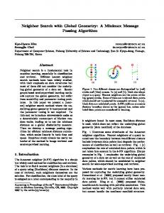
The Sherrington Kirkpatrick (SK) model (Sherrington and Kirkpatrick, 1975) is a mean-field version of the Edward-Anderson Model (Edwards and Anderson, 1975) and it is defined by a system of N Ising spins σ = (σ1 , σ2 , . . . , σN ) taking values ±1 placed on the vertices of a lattice. In the SK mean field description the model is fully connected: every spin interacts with everybody else, and the couplings Jij are chosen independent and identically distributed according to a gaussian probability distribution, such that, the probability distribution of the whole couplings reads   X Y N 2 Jij P (J) = P (Jij ) ∝ exp − . 2 i 0, or to 1 otherwise), and the SAT formula is reduced (decimated) using this individual assignment. The method is repeated until all the variables are assigned, or until the BP fails to converge. The probability that BP-guided decimation results in a SAT assignment is shown in Figure 10, for several values of α and for K = 3, 4. Note that for 3-SAT the decimation method returns a SAT assignemt almost everytime the BP iteration converges (that is, for α . 3.85). In contrast, for 4-SAT BP-guided decimation finds SAT assignments for α . 9.25, while BP converges most of the time for α . 10.3 (a value that is larger than the conjectured SAT-UNSAT threshold, αs (4) ≈ 10.93). This numerical experiment shows that something goes wrong when α is large enough. It also shows that 4-SAT is qualitatively different from 3-SATs; what makes BP fail at large α differs depending on the K we consider. For K = 3 the BP fixed point becomes unstable at around αst ≈ 3.86, which leads to errors in decimations. [short sketch on how to determine

18

K=3

K=4 1

N = 10000 N = 5000 N = 5000, dec.

probability of convergence

1

0 3.5

4.0

0

αs

9.0

clause density, α

αs

11.0

clause density, α

Figure 10. Empirical probability that the BP algorithm converges to a fixed point, as a function of the the clause density, for 3-SAT (left) and 4-SAT (right). The estimate is based on 100 instances with the number of variables indicated in the legend. Squares indicate emprirical probability that BP-guided decimation finds a SAT assignment, using 100 instances with 5000 variables each. The vertical dashed line is located at the SAT-UNSAT threshold αs . Parameters of the decimation: δ = 10−2 , tmax = 103 . Figures adapted from (Mézard and Montanari, 2009).

stability: entropic factor vs correlation decay] For K = 4, in contrast, the BP fixed point remains stable but does not lead to the correct marginals because the 1RSB condensation threshold αc is crossed.

The 1RSB cavity method We could proceed with the strategy outlined in Section , using the BP approximation in the auxiliary model in order to estimate the complexity function Σ(f ). This can be done, but it gets complicated because we need to operate on probability functions (the Bethe measures) rather than on simple real numbers. If we just want to compute the entropy to find whether or not there exist solutions, we can take a shortcut, based on the min-sum algorithm. Instead of computing the marginals of the distribution in Eq. (30), we consider the problem of minimizing the following cost (energy) function E(x) =

M X

Ea (x∂a ).

(47)

a=1

where Ea (x∂a ) = 0 if clause a is satisfied by the assignment x = (x1 , . . . , xN ), while Ea (x∂a ) = 0 otherwise. The two problems are mapped onto each other through ψa (x∂a ) = e−βEa (x∂a ) , with β > 0. The particular choice of the factor ψa as the indicator function of clause Ca , Eq. (31), corresponds to the zero temperature limit β → ∞. In this formulation, the SAT-UNSAT threshold αs (K) is identified as the value α above which the probability of having a configuration with ground state energy, E(x) = 0, vanishes. We will estimate the ground state density with the cavity method. For this we need to adapt the message-passing rules, Eqs. (32)–(33), in two steps. First we need to compute max-marginals, rather than marginals. This is a straightforward step that consists of replacing sums with maximizations, and leads to the so-called max-product update rules   Y (t) (t) m ˆ a→i (xi ) ∼ mk→a (xk ) , (48) = max ψa (x∂a ) x∂a\i

(t+1) mi→a (xi )

∼ =

Y

k∈∂a\i (t) m ˆ b→i (xi ).

(49)

b∈∂i\a

Second, we express these update rules in terms of the energy E(x), which amounts to taking the logarithm of Eqs. 48–(49). The resulting algorithm is the so-called min-sum algorithm:   X (t) (t) (t) ˆ Ea→i (xi ) = min Ea (x∂a ) + Ek→a (xk ) + Cˆa→i , (50) x∂a\i

(t+1) Ei→a (xi )

=

X

k∈∂a\i

ˆ (t) (xi ) E b→i

(t)

+ Ci→a .

b∈∂i\a

19

(51)

The fixed point of these equations are known as the energetic cavity equations. In the same way that the max-product marginals are defined up to a multiplicative constant, min-sum (t) (t) messages are defined up to an overall additive constant. We set the constants Ci→a and Cˆa→i (t+1) ˆ (t) (xi ) = 0. With this arrangement, all energies so that minxi Ei→a (xi ) = 0 and minxi E i→a are relative to the ground-state energy.

Warning Propagation The fact that the energy function, Eq. (47), counts the number of violated constraints allows us to simplify the min-sum updates given by Eqs. (50)–(51). It can be shown that, if messages ˆ (0) are either 0 or 1, the subsequent values of E ˆ (t) obtained from are initialized so that E a→i the min-sum updates will also be either 0 or 1 (see (Mézard and Montanari, 2009)). As a consequence of this property, instead of keeping track of the variable-to-node messages Ei→a (·), we will only bother to use the projections on {0, 1}, Ei→a (xi ) = min{1, Ei→a (xi )}. The update rules become   X (t) (t) ˆ (t) (xi ) = min Ea (x∂a ) + E E (x ) + Cˆa→i , a→i k→a k x∂a\i

(t+1) Ei→a (xi )

 = min 1,

(52)

k∈∂a\i

 (t) (t) ˆ Eb→i (xi ) + Ci→a .

X

(53)

b∈∂i\a

This simplified min-sum algorithm with update equations (52)–(53) is called the warning propagation algorithm. The name stems from the interpretation of Ei→a as a warning: Ei→a = 1 means that, according to the set of constraints b ∈ ∂i\a, the i-th variable should not take the value xi ; analogously, Ei→a = 0 means that, according to the set of constraints b ∈ ∂i\i, the i-th variable has green light to take the value xi . The main advantage of warning propagation is that messages are are either 0 or 1, rather than distributions. Because our problem involves binary variables and hard constraints, the messages of the 1RSB cavity equations are triples: (Qia (0), Qia (1), Qia (∗)) for variable-to-function messages ˆ ai (0), Q ˆ ai (1), Q ˆ ai (∗)) for function-to-variable messages. In the case of K-satisfiability, and (Q ˆ ai (1) is necessarily 0; if Jai = 1 these messages can be simplified further: if Jai = 0 then Q ˆ then Qai (0) must be 0. This is because a ‘0’ message mans that the constraint a forces xi to take the value 0 in order to minimize the system’s energy. In K-SAT this can happen only if Jai = 0, because xi = 0 is the value that satisfies a. An analogous argument applies for the ‘1’ message. The bottom-line is that function-to-variable messages can be parametrized by a ˆ ai (0) if Jai = 0 and Q ˆ ai (1) if Jai = 1, and single real number. We take this number to be Q ˆ denote it simply by Qai . Similarly, we can use a parametrization for the variable-to-function message Qia (·) that takes into account the value of Jai . We denote by Qia (0), Qia (∗), and Qia (1) the three possible type of messages: m(1) > m(0) = 0, m(0) = m(1) = 0, and m(0) > m(1) = 0, respectively. We then define, if Jai = 0, QSia ≡ Qia (0), Q∗ia ≡ Qia (∗), and QU ia ≡ Qia (1). Conversely, if Jai = 1, we have QSia ≡ Qia (1), Q∗ia ≡ Qia (∗), and QU ≡ Q (0). The interpretation of the ia ia new defined variables is as follows
QSia = Pr xi is forced to satisfy a by b ∈ Sia ,
QU ia = Pr xi is forced to violate a by b ∈ Uia ,
Q∗ia = Pr xi is not forced by b ∈ Sia ∪ Uia ,
ˆ ai = Pr xi is forced by clause a to satisfy a . Q At this point we could derive the explicit 1RSB equations in terms of the messages QS , ˆ Another option is to use the above interpretation of the messages to guess Q , Q∗ , and Q. the 1RSB cavity equations. Note first that clause a forces variable xi to satisfy a only when all the other variables involved in a are forced (by some other clause) not to satisfy a. This can be stated as Y ˆ ai = Q QU ja . U

j∈∂a\i

20

Let’s define ΩS and ΩU as, respectively, the subset of clauses Sia and Uia that send a warning. For concreteness, let’s pick the variable node i and assume that Jia = 0 (the opposite case leads to identical equations). In that case, Sia is the subset b ∈ ∂i\a for which Jib = 0, while Uia is the remaining set of neighbors except a for which Jib = 1. Let’s also assume that the clauses ΩS ⊆ Sia and ΩU ⊆ Uia force the variable node i to take the value xi that satisfies them. It follows that xi is forced to satisfy a if |ΩS | > |ΩU |, and it is forced to violate a if |ΩS | < |ΩU |; xi is not forced if |ΩS | = |ΩU |. The energy shift equals the number of ‘forcing’ clauses in ∂i\a that are violated when xi is set to satisfy the largest number of clauses. This leads to min(|ΩS |, |ΩU |) violated clauses. The resulting 1RSB message passing algorithm, also known as Survey Propagation equations, reads X Y Y S ∼ ˆ bi ˆ bi ), QU e−y|Ω | Q (1 − Q (54) ia = |ΩU |>|ΩS |

QSia ∼ =

b∈ΩU ∪ΩS U

X

e−y|Ω

|

|ΩS |>|ΩU |

Q∗ia ∼ =

b∈Ω / U ∪ΩS

e−y|Ω

|ΩU |=|ΩS |

|

Y b∈ΩU ∪ΩS

Y

ˆ bi Q

b∈ΩU ∪ΩS U

X

Y

ˆ bi ), (1 − Q

(55)

ˆ bi ). (1 − Q

(56)

b∈Ω / U ∪ΩS

Y

ˆ bi Q

b∈Ω / U ∪ΩS

energetic complexity, Σ

S ∗ The overall normalization is fixed by the condition QU ia + Qia + Qia = 1. These equations are not much more complicated to solve than those for BP. Like in the BP equations, we can ˆ ai , Qia } for a given instance, or, use Eqs. (54)–(56) to find the fixed point of the messages {Q rather, we can do statistical analysis. In the latter case, we can compute with population ˆ ai ) and P (QU , QS , Q∗ ). We can then compute the Bethe-free dynamics the probabilities P (Q ia ia ia energy, and then the Legendre transform of the resulting formula, from which we obtain the complexity as a function of the energy. We get Figure 11 From the figure we see that

0.02

α = 4.1 α = 4.2 α = 4.3 0

0

0.005

energy density, e

Figure 11. Energetic complexity density versus energy density for the 3-SAT problem, and for three different clause densities, indicated in the legend. α = 4.3 we get a certain number of contradictions (given by the finite energy at Σ = 0, i.e., the intersection with the abscissa). The number of contradictions decreases as we reduce α, until contradictions vanish. This happens when the value of α is such that the curve crosses the origin of the Σ vs energy curve, which is approximately α ≈ 4.2667. This is the prediction for the SAT-UNSAT threshold. An analogous derivation for the 4-SAT problem leads to the estimate α ≈ 9.667.

References Almeida, JRL De and Thouless, David J. (1978). Stability of the Sherrington-Kirkpatrick solution of a spin glass model. J. Phys. A, 11(5), 983. Edwards, Samuel Frederick and Anderson, Phil W (1975). Theory of spin glasses. J. Phys. F , 5(5), 965. Mézard, Marc and Montanari, Andrea (2009). Information, Physics, and Computation. Oxford University Press. Mézard, Marc and Mora, Thierry (2009). Constraint satisfaction problems and neural networks: A statistical physics perspective. J. Physiol.-Paris, 103(1), 107–113.

21

Mézard, Marc and Parisi, Giorgio (2001). The Bethe lattice spin glass revisited. Euro. Phys. J. B, 233, 217–233. Mézard, Marc and Parisi, Giorgio (2003). The cavity method at zero temperature. J. Stat. Phys., 111(April). Mézard, Marc, Parisi, Giorgio, and Virasoro, Miguel Ángel (1986). SK model: The replica solution without replicas. Europhys. Lett, 1(2), 77–82. Parisi, Giorgio (1979). Infinite number of order parameters for spin-glasses. Phys. Rev. Lett., 43(23), 1754. Parisi, Giorgio (1980). The order parameter for spin glasses: A function on the interval 0-1. J. Phys. A, 13(3), 1101. Sherrington, D. and Kirkpatrick, S. (1975, December). Solvable Model of a Spin-Glass. Phys. Rev. Lett., 35, 1792–1796. Thouless, DJ, Anderson, PW, and Palmer, RG (1977). Solution of ’solvable model of a spin glass’. Philos. Mag., 35(3), 593–601. Touchette, Hugo (2009). The large deviation approach to statistical mechanics. Phys. Rep., 478(1-3), 1–69.

22