The piecewise-linear Galerkin finite element method of Chapter 1 can be ... The
finite element method appeared to converge as O(h) in strain energy and O(h2).
Chapter 2 One-Dimensional Finite Element Methods 2.1 Introduction The piecewise-linear Galerkin �nite element method of Chapter 1 can be extended in several directions. The most important of these is multi-dimensional problems� however, we'll postpone this until the next chapter. Here, we'll address and answer some other questions that may be inferred from our brief encounter with the method. 1. Is the Galerkin method the best way to construct a variational principal for a partial di�erential system? 2. How do we construct variational principals for more complex problems? Speci�cally, how do we treat boundary conditions other than Dirichlet? 3. The �nite element method appeared to converge as O(h) in strain energy and O(h2) in L2 for the example of Section 1.3. Is this true more generally? 4. Can the �nite element solution be improved by using higher-degree piecewisepolynomial approximations? What are the costs and bene�ts of doing this? We'll tackle the Galerkin formulations in the next two sections, examine higher-degree piecewise polynomials in Sections 2.4 and 2.5, and conclude with a discussion of approximation errors in Section 2.6.
2.2 Galerkin's Method and Extremal Principles \For since the fabric of the universe is most perfect and the work of a most wise creator, nothing at all takes place in the universe in which some rule of maximum or minimum does not appear." 1
2
One-Dimensional Finite Element Methods - Leonhard Euler
Although the construction of variational principles from di�erential equations is an important aspect of the �nite element method it will not be our main objective. We'll explore some properties of variational principles with a goal of developing a more thorough understanding of Galerkin's method and of answering the questions raised in Section 2.1. In particular, we'll focus on boundary conditions, approximating spaces, and extremal properties of Galerkin's method. Once again, we'll use the model two-point Dirichlet problem
L�u] := ;�p(x)u ] + q(x)u = f (x)
0 0 and q � 0, we have A(v v) � 0� thus, u minimizes (2.2.3). In order to prove the converse, assume that u(x) minimizes (2.2.3) and use (2.2.4) to obtain
I �u] � I �u + �v]: For a particular choice of v(x), let us regard I �u + �v] as a function �(�), i.e., I �u + �v] := �(�) = A(u + �v u + �v) ; 2(u + �v f ): A necessary condition for a minimum to occur at � = 0 is � (0) = 0� thus, di�erentiating � (�) = 2�A(v v) + 2A(v u) ; 2(v f ) and setting � = 0 � (0) = 2�A(v u) ; (v f )] = 0: Thus, u is a solution of (2.2.2a). The following corollary veri�es that the minimizing function u is also unique. Corollary 2.2.1. The solution u of (2.2.2a) (or (2.2.3)) is unique. Proof. Suppose there are two functions u1 u2 2 H01 satisfying (2.2.2a), i.e., A(v u1) = (v f ) A(v u2) = (v f ) 8v 2 H01: 0
0
0
Subtracting
A(v u1 ; u2) = 0 8v 2 H01: Since this relation is valid for all v 2 H01, choose v = u1 ; u2 to obtain A(u1 ; u2 u1 ; u2) = 0: If q(x) > 0, x 2 (0 1), then A(u1 ; u2 u1 ; u2) is positive unless u1 = u2. Thus, it su�ces to consider cases when either (i) q(x) � 0, x 2 �0 1], or (ii) q(x) vanishes at
isolated points or subintervals of (0 1). For simplicity, let us consider the former case. The analysis of the latter case is similar. When q(x) � 0, x 2 �0 1], A(u1 ; u2 u1 ; u2) can vanish when u1 ; u2 = 0. Thus, u1 ; u2 is a constant. However, both u1 and u2 satisfy the trivial boundary conditions (2.2.1b)� thus, the constant is zero and u1 = u2. 0
0
2.2. Galerkin's Method and Extremal Principles
5
Corollary 2.2.2. If u w are smooth enough to permit integrating A(u v) by parts then
the minimizer of (2.2.3), the solution of the Galerkin problem (2.2.2a), and the solution of the two-point boundary value problem (2.2.1) are all equivalent. Proof. Integrate the di�erentiated term in (2.2.3) by parts to obtain
I �w] =
Z1
�;w(pw ) + qw2 ; 2fw]dx + wpw j10: 0
0
0
0
The last term vanishes since w 2 H01� thus, using (2.2.1a) and (2.2.2b) we have
I �w] = (w L�w]) ; 2(w f ):
(2.2.5)
Now, follow the steps used in Theorem 2.2.1 to show
A(v u) ; (v f ) = (v L�u] ; f ) = 0
8v 2 H01
and, hence, establish the result. The minimization problems (2.2.3) and (2.2.5) are equivalent when w has su�cient smoothness. However, minimizers of (2.2.3) may lack the smoothness to satisfy (2.2.5). When this occurs, the solutions with less smoothness are often the ones of physical interest.
Problems
1. Consider the \stationary value" problem: �nd functions w(x) that give stationary values (maxima, minima, or saddle points) of
I �w] =
Z1
F (x w w )dx
(2.2.6a)
0
0
when w satis�es the \essential" (Dirichlet) boundary conditions
w(0) = �
w(1) = �:
(2.2.6b)
Let w 2 HE1 , where the subscript E denotes that w satis�es (2.2.6b), and consider comparison functions of the form (2.2.4) where u 2 HE1 is the function that makes I �w] stationary and v 2 H01 is arbitrary. (Functions in H01 satisfy trivial versions of (2.2.6b), i.e., v(0) = v(1) = 0.) Using (2.2.1) as an example, we would have
F (x w w ) = p(x)(w )2 + q(x)w2 ; 2wf (x) 0
0
� = � = 0:
Smooth stationary values of (2.2.6) would be minima in this case and correspond to solutions of the di�erential equation (2.2.1a) and boundary conditions (2.2.1b).
6
One-Dimensional Finite Element Methods Di�erential equations arising from minimum principles like (2.2.3) or from stationary value principles like (2.2.6) are called Euler-Lagrange equations. Beginning with (2.2.6), follow the steps used in proving Theorem 2.2.1 to determine the Galerkin equations satis�ed by u. Also determine the Euler-Lagrange equations for smooth stationary values of (2.2.6).
2.3 Essential and Natural Boundary Conditions The analyses of Section 2.2 readily extend to problems having nontrivial Dirichlet boundary conditions of the form
u(0) = �
u(1) = �:
(2.3.1a)
In this case, functions u satisfying (2.2.2a) or w satisfying (2.2.3) must be members of H 1 and satisfy (2.3.1a). We'll indicate this by writing u w 2 HE1 , with the subscript E denoting that u and w satisfy the essential Dirichlet boundary conditions (2.3.1a). Since u and w satisfy (2.3.1a), we may use (2.2.4) or the interpretation of �v as a variation shown in Figure 2.2.1, to conclude that v should still vanish at x = 0 and 1 and, hence, belong to H01. When u is not prescribed at x = 0 and/or 1, the function v need not vanish there. Let us illustrate this when (2.2.1a) is subject to conditions
u(0) = �
p(1)u (1) = �:
(2.3.1b)
0
Thus, an essential or Dirichlet condition is speci�ed at x = 0 and a Neumann condition is speci�ed at x = 1. Let us construct a Galerkin form of the problem by again multiplying (2.2.1a) by a test function v, integrating on �0 1], and integrating the second derivative terms by parts to obtain
Z
1
v�;(pu ) + qu ; f ]dx = A(v u) ; (v f ) ; vpu j10 = 0: 0
0
0
0
(2.3.2)
With an essential boundary condition at x = 0, we specify u(0) = � and v(0) = 0� however, u(1) and v(1) remain unspeci�ed. We still classify u 2 HE1 and v 2 H01 since they satisfy, respectively, the essential and trivial essential boundary conditions speci�ed with the problem. With v(0) = 0 and p(1)u (1) = � , we use (2.3.2) to establish the Galerkin problem for (2.2.1a, 2.3.1b) as: determine u 2 HE1 satisfying 0
A(v u) = (v f ) + v(1)�
8v 2 H01:
(2.3.3)
2.3. Essential and Natural Boundary Conditions
7
Let us reiterate that the subscript E on H 1 restricts functions to satisfy Dirichlet (essential) boundary conditions, but not any Neumann conditions. The subscript 0 restricts functions to satisfy trivial versions of any Dirichlet conditions but, once again, Neumann conditions are not imposed. As with problem (2.2.1), there is a minimization problem corresponding to (2.2.3): determine w 2 HE1 that minimizes
I �w] = A(w w) ; 2(w f ) ; 2w(1)�:
(2.3.4)
Furthermore, in analogy with Theorem 2.2.1, we have an equivalence between the Galerkin (2.3.3) and minimization (2.3.4) problems.
Theorem 2.3.1. The function u 2 HE1 that minimizes (2.3.4) is the one that satis�es (2.3.3) and conversely.
Proof. The proof is so similar to that of Theorem 2.2.1 that we'll only prove that the function u that minimizes (2.3.4) also satis�es (2.3.3). (The remainder of the proof is stated as Problem 1 as the end of this section.) Again, create the comparison function
w(x) = u(x) + �v(x)�
(2.3.5)
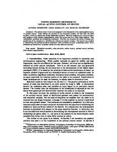
however, as shown in Figure 2.3.1, v(1) need not vanish. By hypothesis we have u, w w(x) ε v(x)
α u(x) x 0
1
Figure 2.3.1: Comparison function w(x) and variation �v(x) when Dirichlet data is prescribed at x = 0 and Neumann data is prescribed at x = 1.
I �u] � I �u + �v] = �(�) = A(u + �v u + �v) ; 2(u + �v f ) ; 2�u(1) + �v(1)]�:
8
One-Dimensional Finite Element Methods
Di�erentiating with respect to � yields the necessary condition for a minimum as � (0) = 2�A(v u) ; (v f ) ; v(1)� ] = 0� thus, u satis�es (2.3.3). 0
As expected, Theorem 2.3.1 can be extended when the minimizing function u is smooth. Corollary 2.3.1. Smooth functions u 2 HE1 satisfying (2.3.3) or minimizing (2.3.4) also satisfy (2.2.1a, 2.3.1b). Proof. Using (2.2.2c), integrate the di�erentiated term in (2.3.3) by parts to obtain
Z
1
v�;(pu ) + qu ; f ]dx + v(1)�p(1)u (1) ; � ] = 0 0
0
0
0
8v 2 H01:
(2.3.6)
Since (2.3.6) must be satis�ed for all possible test functions, it must vanish for those functions satisfying v(1) = 0. Thus, we conclude that (2.2.1a) is satis�ed. Similarly, by considering test functions v that are nonzero in just a small neighborhood of x = 1, we conclude that the boundary condition (2.3.1b) must be satis�ed. Since (2.3.6) must be satis�ed for all test functions v, the solution u must satisfy (2.2.1a) in the interior of the domain and (2.3.1b) at x = 1. Neumann boundary conditions, or other boundary conditions prescribing derivatives (cf. Problem 2 at the end of this section), are called natural boundary conditions because they follow directly from the variational principle and are not explicitly imposed. Essential boundary conditions constrain the space of functions that may be used as trial or comparison functions. Natural boundary conditions impose no constraints on the function spaces but, rather, alter the variational principle.
Problems
1. Prove the remainder of Theorem 2.3.1, i.e., show that functions that satisfy (2.3.3) also minimize (2.3.4). 2. Show that the Galerkin form (2.2.1a) with the Robin boundary conditions p(0)u (0) + �0u(0) = �0 p(1)u (1) + �1u(1) = �1 is: determine u 2 H 1 satisfying A(v u) = (v f ) + v(1)(�1 ; �1u(1)) ; v(0)(�0 ; �0u(0)) 8v 2 H 1: Also show that the function w 2 H 1 that minimizes I �w] = A(w w) ; 2(w f ) ; 2�1w(1) + �1w(1)2 + 2�0w(0) ; �0w(0)2 is u, the solution of the Galerkin problem. 0
0
2.4. Piecewise Lagrange Polynomials
9
3. Construct the Galerkin form of (2.2.1) when
p(x) = 12 ifif 01=�2 �x 0, depending on p, such that
ku ; U k0 � Cphp+1ku(p+1)k0
(2.6.18a)
ku ; U k1 � Chppku(p+1)k0:
(2.6.18b)
and where h satis�es (2.6.12c). Proof. The analysis follows the one used for linear polynomials.
Problems 1. Choose a hierarchical polynomial (2.5.3) on a canonical element �;1 1] and show how to determine the coe�cients cj , j = ;1 1 2 : : : p, to solve the interpolation problem (2.6.7).
Bibliography �1] M. Abromowitz and I.A. Stegun. Handbook of Mathematical Functions, volume 55 of Applied Mathematics Series. National Bureau of Standards, Gathersburg, 1964. �2] R.L. Burden and J.D. Faires. Numerical Analysis. PWS-Kent, Boston, �fth edition, 1993. �3] G.F. Carey and J.T. Oden. Finite Elements: A Second Course, volume II. Prentice Hall, Englewood Cli�s, 1983. �4] R. Courant and D. Hilbert. Methods of Mathematical Physics, volume 1. WileyInterscience, New York, 1953. �5] C. de Boor. A Practical Guide to Splines. Springer-Verlag, New York, 1978. �6] E. Isaacson and H.B. Keller. Analysis of Numerical Methods. John Wiley and Sons, New York, 1966. �7] B. Szab�o and I. Babuska. Finite Element Analysis. John Wiley and Sons, New York, 1991.
31