Compositional Security Modelling Structure, Economics, and Behaviour Tristan Caulfield1 , David Pym1 , and Julian Williams2 1
Department of Computer Science University College London {t.caulfield,d.pym}@ucl.ac.uk 2 Business School University of Durham
[email protected]
Abstract. Security managers face the challenge of formulating and implementing policies that deliver their desired system security postures — for example, their preferred balance of confidentiality, integrity, and availability — within budget (monetary and otherwise). In this paper, we describe a security modelling methodology, grounded in rigorous mathematical systems modelling and economics, that captures the managers’ policies and the behavioural choices of agents operating within the system. Models are executable, so allowing systematic experimental exploration of the system-policy co-design space, and compositional, so managing the complexity of large-scale systems.
1
Introduction
Security managers in all types of organizations must routinely choose policies and technologies that protect the business-critical infrastructure of their systems. These choices are constrained by both regulatory and economic circumstances and managers necessarily must make trade-offs between security and such operational constraints. When faced with analysing these trade-offs security managers currently have very limited tools to aid them in systematic decision-making. Consequently, managers must rely on their own judgement when selecting their implementation choices. While this approach does not necessarily lead to poor decision-making, it does have some inherent weaknesses. Decisions made in this fashion may or may not be optimal, but typically cannot be shown to be optimal, and their relative effectiveness and value cannot be established, because the manager has no rigorous means of comparison with other approaches. Moreover, any decisions taken by the manager cannot be shared in a meaningful way with other stakeholders, such as operations managers, finance managers, or senior strategists. Our hypothesis, supported by a body of exploratory (e.g., [1, 2]) and theoretical (e.g., [13, 14]) work, is that a specific combination of mathematical systems modelling of the structure and dynamics of organizations and their behaviour and economic modelling of their security policy design and decision-making can deliver a framework within which the consequences of security policy and technology co-design decisions
can be predicted and explored experimentally. The security systems of interest are often complex assemblies of agents, be they software or human, policies, and technology. Handling substantive system complexity is challenging for reasoning tools, as has been observed, for example, in the world of formal methods in software engineering. The lesson that has been learned is that such tools must be compositional. In Section 2, we summarize the system modelling theory, its implementation in the Julia language, and explain our use of production and utility functions to model policies and decision-making in the context of our experimental methodology. In Section 3, we describe two examples of system security policies and present a range of experimental results. Section 4 explains how our approach allows models to be composed systematically. We summarize our contribution and discuss further work in Section 5.
2 2.1
Systems and Security Modelling System Modelling
The notion of process has been explored in some detail by the semantics community. Concepts like resource and location have, however, usually been treated as second class ([18] is a partial exception). Whilst there are some good theoretical reasons to do this, in [5] we explore what can be gained by developing an approach in which the structures present in modelling languages are given a rigorous theoretical treatment as first-class citizens. We ensure that each component — location, resource, and process — is handled compositionally. In addition to the structural components of models, we consider also the environment within which a system exists: Environment: All systems exist within an external environment, which is typically treated as a source of events that are incident upon the system rather than being explicitly stated. Mathematically, environments are represented stochastically, using probability distributions that are sampled in order to provide such events [5]. The key structural components are considered, drawing upon classical distributed systems theory — see, for example, [7] — below. Location: Places are connected by (directed) links. Locations may be abstracted and refined provided the connectivity of the links and the placement of resources is respected. Mathematically, the axioms for locations [5] are satisfied by various graphical and topological structures, including simple directed graphs and hyper-graphs [5]; Resource: The notion of resource captures the components of the system that are manipulated by its processes (see below). Resources include things like computer memory, system operating staff, or system users, as well as money. Conceptually, the axioms of resources are that they can be combined and compared. We model this notion using (partial commutative) resource monoids [19, 5]: structures R = (R, v, ◦, e) with carrier set R, preorder v, and partial binary composition ◦ with unit e, and which satisfies the bifunctoriality condition: R v R0 and S v S 0 and R ◦ S is defined implies R0 ◦ S 0 is defined and R ◦ S v R0 ◦ S 0 , for all R, S, R0 , S 0 ∈ R. Process: The notion of process captures the (operational) dynamics of the system. Processes manipulate resources in order to deliver the system’s intended services. Mathematically, we use algebraic representation of processes based on the ideas in [17], integrated with the notions of resource and location [5].
Let Act be a commutative monoid of actions, with multiplication written as juxtaposition and unit 1. Let a, b ∈ Act, etc., so that their multiplication is written ab, etc.. The execution of models based on these concepts, as formulated in [5], is described by a transition system with a basic structural operational semantics judgement [17] of the a form L, R, E −→ L0 , R0 , E 0 , which is read as ‘the occurrence of the action a evolves the process E, relative to resources R at locations L, to become the process E 0 , which then evolves relative to resources R0 at locations L0 ’. The meaning of this judgement is given by a structural operational semantics [17]. The basic case, also know as ‘action prefix’, is the rule
a
L, R, a : E −→ L0 , R0 , E 0
µ(L, R, a) = (L0 , R0 ).
Here µ is a ‘modification’ function from locations, resources, and actions (assumed to form a monoid) to locations and resources that describes the evolution of the system when an action occurs. Suppressing locations for now, a partial function µ : Act × R → R is a modification if it satisfies the following conditions for all a, b, R, S: µ(1, R) = R; if R ◦ S and µ(a, R) ◦ µ(b, S) are defined, then µ(ab, R ◦ S) = µ(a, R) ◦ µ(b, S). There are also rules giving the semantics to combinators for concurrent composition, choice, and hiding — similar to restriction in SCCS and other process algebras (e.g., [17]) — as well for recursion. For example, the rule for synchronous concurrent composition of processes is a
L, R, E −→ L0 , R0 , E 0 ab
b
M, S, F −→ M 0 , S 0 , F 0
,
L · M, R ◦ S, E × F −→ L0 · M 0 , R0 ◦ S 0 , E 0 × F 0 where we presume, in addition to the evident monoidal compositions of actions and resources, a composition on locations (here written as ·). The rules for the other combinators, with suitable coherence conditions on the modification functions, follow similar patterns [5]. Note that our choice of a synchronous calculus retains the ability to model asynchrony [17, 8] (this doesn’t work the other way round). For another example, a key process construct for this paper is non-deterministic choice or sum: ai L, R, Ei −→ L0 , R0 , E 0 i = 1, 2. ai L, R, E1 + E2 −→ L0 , R0 , E 0 For example, suppressing location and resource, a process (a : E) + (b : F ) + (c : G) will evolve to become E, F , or G depending on the next action being a, b, or c. Along with the transition system described here comes, in the sense of Hennessy– Milner [11, 5], a modal logic [5] with basic judgement L, R, E |= φ, where the proposition φ expresses a property of the process E executing with respect to resources R at location L. This logic includes, in addition to the kinds of connectives and modalities usually encounter in process logics, a number of substructural connectives and modalities that are helpful in reasoning compositional about resource-bounded systems. This modal logic can also be extended to the stochastic world. An account of this logic and its extensions is beyond our present scope, but will be of interest in further work.
2.2
Representing the Concepts in Julia
As discussed in Section 2.1, our mathematical modelling framework employs the classical distributed systems concepts of location, resource, process, and environment. In this work, we represent these concepts using the Julia language [15, 3]. The language is designed for scientific and numeric computing and also has support for co-routines, making it ideal for process-based simulation. We represent the modelling concepts in Julia as follows: – Environment is handled by Julia’s ability to sample probability distributions; – Locations are instances of a type with associated links to other locations (and so are graph-like) and associated resources; – Resources are instances of a type on which algebraic operations (such as those required for a resource monoid) can be defined; – Processes are represented by co-routines that provide us with the necessary constructs for concurrent execution and choice. The modelling language Gnosis [6, 5] provides, by construction, a reference implementation for the mathematical constructs explained in Section 2.1. However, Julia provides a superior programming environment that is convenient for practical modelling. Models constructed in Julia are executed in order to explore the consequences of system- and security policy-design decisions, including representations of the behaviour of agents (see subsequent sections). Julia models are designed in layers. At the bottom, they provide functionality for constructing locations, resources, and processes, and executing the latter. On top of this is code for agents and decision-making within the model (again, see subsequent sections). Finally, there is functionality specific to security simulations. This includes a library of standard components, such as implementations of access control mechanisms, that can be configured as required for a particular model. The full code for the models presented in this paper is available at http://www. cs.ucl.ac.uk/staff/D.Pym/FTNCTC-Julia-code.pdf.
2.3
Productivity and Utility
The processes described above provide a representation for the agents that inhabit and explore a security system. As they explore the system, agents make decisions about their trajectory through the systems. Decisions are made by agents at specific locations within the system and may depend on the resources that are available at those locations. Each decision that is made involves a choice between competing alternatives that are available to the agent at its location, given the resources that are available at that location. In economics, this situation can be described using production functions [10]. A leading example is provided by the Cobb-Douglas production function (e.g., [4] for an innovative, and similar, use of production functions in economics). We show how to employ Cobb-Douglas production functions in a way that supports the composition of models (see Section 4).
In its simplest form, the (real-valued) Cobb-Douglas production function, as used in this setting,3 expresses the value D of a decision in terms of the values, X and Y , of two alternatives whose relative likelihood of occurrence is weighted by parameters α and β such that α + β = 1; that is, D = δ X α Y β , where δ is a scaling factor. Note that the parameter α (and hence β, or vice versa) may be determined stochastically (by sampling a given probability distribution). In general, a model will include a number of agents, all making a number of decisions during the execution of the model. Thus, associated with an execution of the model is a set D of (values of) decisions, written as follows: λi
λ
D = { Di = δi Xi1i1 . . . Xik k | i = 1, . . . , m }. The set D describes the space of decisions taken by agents in the model. In each decision Di , the full space of k choices, Xi1 , . . . , Xik , available is maintained, with their likelihood of being chosen being represent by the λi parameters. Associated with the system is another value; that is, the system manager’s utility. The manager determines a security policy that is intended to deliver target values for certain key attributes of the system. For example, the number of security barrier tailgates, the number of database corruptions, or the up-time of a server. During the operation of the system, the value, V , of an attribute of interest will deviate from its target value, V¯ , by amounts which depend upon the behaviour of the agents within the system, as represented by the decisions, D1 , . . . , Dm , they make, as described above. The manager assigns value to the deviation from target according to a chosen function f ; that is, f (V − V¯ ). The function f is often based on a quadratic or Linex [20] form, and, typically, will incorporate a stochastic component. Overall, the manager will be concerned with a set of such values { Vi | i = 1, . . . n }, and the manager will assign a relative Pnimportance to each deviation from target by a preference, or weighting, wi such that i=1 wi = 1. Thus, the manager’s overall expected utility for the system with the given policy — here the policy is represented by the choice of values of interest, their targets, the functional forms valuing deviation from target, and the preference weightings — is given by the following function: " n # X E[U (D1 , . . . , Dm )] = E wr fr (Vr (D1 , . . . , Dm ) − V¯r ) . r=1
Note that here we have expected utility, deriving from the presence of stochastic components in the parameters α and β and the functions fi . Note also that in this set-up a separation is maintained between the decisions made by the agents and the manager’s overall utility calculation. Moreover, the dependency 3
In a standard economic setting using such a production function, X and Y are inputs (typically capital and labour), δ is the return to scale, and α and β are the elasticities of X and Y . The constraint that α +β = 1 generally yields tractable solutions. Our use of a production function inspired by Cobb-Douglas to describe security decisions amounts to an hypothesis that security decision-making is log linear (cf. [9], in which exponential decay in losses amounts to this assumption).
of the latter on the former is such that the form of the latter can be used unchanged even if the particular choice of production functions, describing the local value of the agents’ decisions, is changed. Similarly, for a fixed model of the agents’ decisions, described by given production functions, the manager may vary the functional form of the overall utility in order to reflect changes in policy. As with production functions, this use of utility functions supports the composition of models (see Section 4), allowing managers to consider policies for one part of a system in the context of those for other parts. This use of multi-attribute utility theory (see [16] for a detailed account) has been employed as a tool for reasoning in a range of security settings; for example, [12, 14]. 2.4
A Methodology
We have explained how production functions describe the space of decisions that occur in a model and how utility functions describe the system manager’s policy and its value. In an execution of a specific model, a specific agent must make specific choices. In terms of our production functions, this amounts to specific choices of Xi s and corresponding λi s, possibly 0 or 1, with frequency determined by the associated probability distribution. These choices are determined by the agent’s maximizing its own subjective utility. This calculation will be determined by the agent’s state, including its location and execution trajectory. Here we take a maximization given by choose(D) = arg max d∈D
m Y
Xiλdi .
i=1
In terms of the underlying mathematical system model, this choice determines the aca tion a in an evolution L, R, E −→ L0 , R0 , E 0 , where the agent E evolves at location L relative to available resources R — recalling Section 2.1, think of E as a sum of processes, with each choice guarded by a possible action, determined as above. We conduct experiments to explore the co-design of systems and security policies. Specifically, we construct models that encompass the following features: the architecture of the system of interest; its security policy, as represented by the system manager’s overall utility function; and the behaviour of agents (e.g., people) when they interact with the system in the context of its security policy, as represented by the production functions used to describe agents’ decisions. Based on such a model, we explore the following experimental space: for a range of parameter values that describe the configuration of the system and the preferences of its inhabiting agents, we observe the corresponding range of consequent values for the attributes of interest to the system manager (e.g., breaches of policy and system performance) and so are able, at least in principle, to calculate his utility as a basis for refining system design and policy. In full generality, one would conduct full Monte Carlo simulations of the model for given choices of empirical data. Our experimental work, reported in the next section, relies on data collected by the ‘Productive Security’ research project funded by the UK’s GCHQ and EPSRC (grant reference EP/K006517/1) that is currently active at UCL. This project has conducted extensive empirical studies within large organizations to elicit the behaviour of staff in a range of security settings.
The data is collated as a collection of rankings, according to the preferences of subjects, of behavioural options in a range of security scenarios used as basis for semistructured interviews in the organizations.
3
Example Models
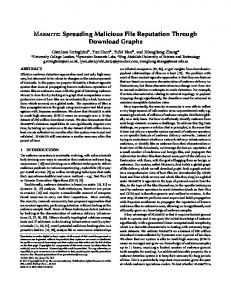
We construct models based on two scenarios: one based on tailgating through the access control to a building and one based on access control through screen locking to personal computers within a shared inner office. The former is richer and explored in much more detail than the latter, which is introduced primarily to facilitate our subsequent discussion of composition in Section 4. This first model looks at tailgating in a business setting. Tailgating is when people without authorization or without the correct credentials follow others through security controls to gain access to a restricted area. In this case, employees arriving at work need an ID badge to gain access to the main office from the foyer. Employees who forget their badges have a choice: to tailgate through security or to gain access through the reception desk. Employees who observe others tailgating also have a choice: to confront the tailgater and send them back to reception, or to ignore them. Other Room
Reception Break Room
Lobby
After Door
Office
Office
Start
Home
Fig. 1. Lobby Tailgating Model
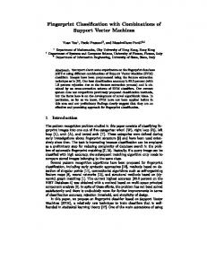
Fig. 2. Inner-office Model No
Yes
Tailgate
Confront
Office
Ignore
Yes
No
Observe Tailgating?
Confronted?
Go through door
No
Reception
Tailgate?
Forgot Card?
Yes
Start
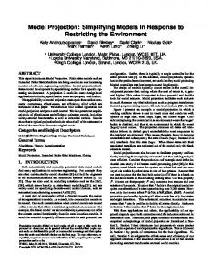
Fig. 3. Agent Processes in the Tailgating Model. Decision Points are Rounded.
Figure 1 shows the locations for the tailgate model, and Figure 3 describes the agents’ processes in this model. The two decision points are shown in rounded boxes. Agents start at home and move to the lobby at work, possibly leaving their access cards, a key resource, behind. Agents that have their access cards proceed directly through the security door. Agents that have forgotten their cards have a decision: to tailgate or to go to reception. If the agents choose to go to reception, they queue up until a receptionist is available, and then proceed through the security door. Agents that tailgate wait until the
door has opened and follow another agent through. Agents in the ‘After Door’ location possibly observe other agents tailgating. If they do, they have a decision to confront the tailgating agents, or to ignore them. Agents that are confronted are assumed to return to reception, queue, and then proceed through the security door. Eventually, agents arrive in the office. In this model, nothing happens once the agents are inside the office; they simply wait there until the end of the day and then leave for home. qLen = queue_length(receptionist) + 1 expectedWait = (qLen * mean(dist_receptionist)) / minutes #get how late we are in minutes late = get_time_of_day(now(agent.proc)) (LEAVE_FOR_WORK_TIME + mean(dist_work_arrival)) late /= minutes #get how late we’ll arrive in office if we queue reception_arrive = late + expectedWait vX_P = 0 if reception_arrive > 0 vX_P += log(reception_arrive ^ 2 + 1) end
vX_S = max(4 - vX_P, 0.0) vX_S *= agent.choice_exponents[SEC] vX_P *= agent.choice_exponents[PROD] vX_I = agent.choice_exponents[INDIV] vX_M = agent.choice_exponents[MAL] exponents = [lamS, lamP, lamI, lamM] #S P I M d_tailgate = [1.0, 3.0, 1.0, 5.0] d_reception = [3.0, 1.0, 1.5, 1.0] choose(agent, exponents, [ Choice(d_tailgate, do_tailgate), Choice(d_reception, do_reception)])
Fig. 4. Julia Code for Tailgating or Reception Decision
Figure 4 shows the Julia code for the choice between tailgating or reception. Here, how much the agent values security or productivity is dependent on whether the agent is early or late to work, and how long the expected wait is for reception. Agents in this model are considered to be individual subjective utility maximizλM ers for each decision D = XSλS XPλP XIλI XM , where the inputs to this production function are security, productivity, individual cognitive cost, and maliciousness, respectively. Here the return to scale is taken to be 1. In this paper, we do not consider the managers’ utility, deferring consideration of policy variation to another occasion. The tables below show some of the output from the (500) simulation runs. The first four columns are parameters: the average time an agent spends at reception, the number of guards present, and the means of the distributions from which agents’ attitudes towards productivity and security are drawn. The remaining columns are outputs, averaged over the simulation runs: the total length of time agents spend waiting for reception, the number of tailgating attempts, success and failures by employees, and the number of malicious tailgating attempts, success, and failures. These attributes reflect 1 1 aspects of confidentiality, integrity, and availability that are of interest to the managers and other agents. Tables 1 and 2 show the output from the tailgating model when there is no guard present and with one guard, respectively. In general, high-value attitudes towards security and low-value attitudes towards productivity result in more agents choosing to queue for reception instead of tailgate; in the opposite case, more agents choose to tailgate. When the attitudes are similar, the agents’ choices are more evenly split. In the presence of guards (Table 2), the total reception time is higher as more tailgating attempts are caught and the agents are sent back to reception. The number of successful malicious tailgating attempts is reduced slightly by a higher attitude towards security. The presence of guardsresults in a significant reduction.
rec mean 60 60 60 60 120 120 120 120
num guards prod mean sec mean rec wait tail tail succ 0 0.2 0.2 2538.14 11.0 3.92 0 0.2 0.8 2376.23 7.02 1.38 0 0.8 0.2 1224.59 12.22 8.52 0 0.8 0.8 1396.19 11.12 5.06 0 0.2 0.2 3888.02 12.56 4.0 0 0.2 0.8 4292.42 12.42 2.04 0 0.8 0.2 1450.58 15.34 9.38 0 0.8 0.8 2047.09 13.8 5.5
tail fail 7.08 5.64 3.7 6.06 8.56 10.38 5.96 8.3
mal tail 1.46 1.44 1.38 1.46 1.44 1.5 1.44 1.66
mal tail succ mal tail fail 0.3 1.16 0.02 1.42 0.7 0.68 0.5 0.96 0.42 1.02 0.18 1.32 0.76 0.68 0.52 1.14
Table 1. Results from Tailgating Model Simulations, without Guard
rec mean 60.0 60.0 60.0 60.0 120.0 120.0 120.0 120.0
num guards prod mean sec mean rec wait tail tail succ 1.0 0.2 0.2 1965.04 9.6 1.3 1.0 0.2 0.8 3331.58 8.24 0.42 1.0 0.8 0.2 995.04 12.8 4.28 1.0 0.8 0.8 1679.81 10.82 1.9 1.0 0.2 0.2 4519.47 13.58 1.54 1.0 0.2 0.8 5214.63 12.96 0.76 1.0 0.8 0.2 1842.76 14.9 3.72 1.0 0.8 0.8 2181.14 12.54 1.56
tail fail 8.3 7.82 8.52 8.92 12.04 12.2 11.18 10.98
mal tail 1.36 1.62 1.46 1.54 1.4 1.58 1.38 1.4
mal tail succ mal tail fail 0.18 1.18 0.06 1.56 0.32 1.14 0.14 1.4 0.16 1.24 0.02 1.56 0.3 1.08 0.14 1.26
Table 2. Results from Tailgating Model Simulations, with Guard
Our preliminary results illustrate that small changes in the attitudes of agents can result in substantial changes in behaviour. For example, looking at the case with no guards and the lower reception time, with strong focus on productivity and less on security, the mean number of tailgate attempts is 12.22, with 8.52 success; when the focus is on security over productivity, this drops to 7.02 attempts and just 1.38 successes. But the total time agents spend queueing for reception nearly doubles. The length of time agents have to spend at reception also impacts on the number of tailgating attempts. Managers employ additional guards in order to further protect confidentiality- and integrity-like attributes. However, the addition of a guard can be seen (Table 2) to have a detrimental effect (see rec wait) on availability-like attributes (e.g., waiting time). The second model looks at whether or not employees lock their screens when they leave their computers and how often unlocked computers are accessed. There are only three locations in this model: the start location, the office, and another room. These are shown in Figure 2. The other room represents all other locations agents might be when they are away from their computers, such as meeting rooms, break rooms, and other parts of the building. While there are fewer locations than in the tailgating model, the agents’ processes are more complicated. Upon arriving in the office, agents have a decision to work or to just walk around. Agents that choose to work find a computer — a resource, located in the office, with locked or unlocked state — wait for a while, and eventually leave to go to the other room. When they leave their computer, they have a choice: to lock the computer or to leave it unlocked. As they are walking to the other room they might encounter another computer that has been left unlocked. They then have another choice: ignore the unlocked computer, lock the computer, or access it. The agents then stay in the other room for some time, and then return to their computers, possibly observing another unlocked computer on the way back.
4
Composition
To describe and reason about complex models, it is convenient to describe them in terms of sub-models of which they are composed. That is, it is convenient, under suitable compatibility conditions, to be able to compose two models to form a more complex model. Independent models can also be considered together, with their sets of decisions and utilities simply being the unions and sums, respectively, to give the overall picture. Whilst such simple combinations of production and utility are desirable, it is necessary to understand the circumstances under which models can be combined in useful ways. This is achieved by describing the interface between two models, so defining what is required for two models to be composable at a specific point. A model can potentially have many interfaces, each with different requirements. We assume here that for each model we can enumerate the locations and their associated directed links that allow resources to be moved in and out of the model by processes. Figure 5 illustrates two models, each of which has various such locations and links. Among these, location K in Model 1 and location L in Model 2, and their associated links, allow the models to be composed at the point indicated by the interface. Model&2& U)lity&U(E1&,&…&,&En)&
K2(
K1( Decisions&D(
&
Interface&
L1(
Reception
L2(
Break Room
Model&1& U)lity&U(D1&,&…&,&Dm)& &Decisions&E(
Fig. 5. Composing Models at an Interface
Lobby
Other Room After Door
Office
Home
Fig. 6. Combined Model
But this description is not yet sufficient to determine a useful composition. For that, we must also require that the agents (processes) that move resources in and out of Model 1 via location K1 must match with the agents (processes) that move resources in and out of Model 2 via location L1 . That is, any agent that is defined in Model 1 and moves resources across the boundary of Model 1 via location K1 must also be defined in Model 2 to move the same resources across the boundary of Model 2 via location L1 . Since the links for the illustrated interface are bidirectional, this condition must hold in both directions, but an interface via locations K2 and L2 (note that their directions are compatible) would require just the one direction. Under these constraints, the detailed formulation of which is beyond the scope of λi λ this short paper, we have that if D = { Di = δi Xi1i1 . . . Xik k | i = 1, . . . , m } and E = λ
λj
{ Ej = δj Yj1j1 . . . Xjk k | j = 1, . . . , n } then the set of decisions for the composite model is simply D ∪ E. Similarly, the overall expected utility for the composite model is simply E[U (D1 , . . . , Dm )] + E[U (E1 , . . . , En )]. We can give a simple illustration of how composition works using the models describe in Section 3. Figure 1 shows the locations and links of the lobby tailgating model. Tailgating is the subject of interest in this model, and what happens once the employees have passed through security into the office is not modelled. Figure 2 shows the locations and links of the office screen-locking model. In this case, the model is designed to study behaviour that occurs within the office.
The office in Figure 1 is a dummy location. Nothing of interest to the model occurs in that location; after getting through security, employees wait there for the end of the work day and then leave. This model can naturally by composed with the office screenlocking model. The dummy office location is removed and replaced with the office location from the second model. Figure 6 shows the resulting locations and links. Tables 3 and 4 show the output from the composite model without and with a guard. These tables have an additional column: the number of times a computer in the office is accessed by a malicious agent. When agents’ attitudes towards security are high and productivity are low, they tend to lock their screens most times when they leave their desks; this results in a low number of malicious accesses. The presence of a guard again reduces the incidences of successful malicious tailgating, and thus also the number of times computers in the office are accessed. rec mean 60 60 60 60 120 120 120 120
num guards prod mean sec mean rec wait tail tail succ 0 0.2 0.2 1995.73 9.56 5.42 0 0.2 0.8 2187.24 8.03 6.93 0 0.8 0.2 929.68 11.58 5.47 0 0.8 0.8 1290.88 9.97 7.65 0 0.2 0.2 3156.48 12.78 5.20 0 0.2 0.8 3355.64 12.50 7.88 0 0.8 0.2 1517.90 14.62 6.15 0 0.8 0.8 1672.00 13.55 8.50
rec mean 60 60 60 60 120 120 120 120
num guards prod mean sec mean rec wait tail tail succ 1 0.2 0.2 1863.38 8.13 1.50 1 0.2 0.8 2677.96 7.67 2.50 1 0.8 0.2 1160.51 12.80 2.53 1 0.8 0.8 1562.94 11.00 3.52 1 0.2 0.2 4126.91 12.85 2.17 1 0.2 0.8 4370.40 12.17 3.37 1 0.8 0.2 1981.08 15.50 2.48 1 0.8 0.8 2161.73 13.37 3.85
tail fail 4.14 1.10 6.12 2.32 7.58 4.62 8.47 5.05
mal tail 1.30 1.40 1.48 1.45 1.45 1.33 1.43 1.32
mal tail succ mal tail fail access 0.52 0.78 8.76 0.65 0.75 0.00 0.40 1.08 10.48 0.65 0.80 9.08 0.57 0.88 9.05 0.67 0.67 0.00 0.50 0.93 13.63 0.82 0.50 10.87
Table 3. Results from Composite Model Simulations, without Guard tail fail 6.63 5.17 10.27 7.48 10.68 8.80 13.02 9.52
mal tail 1.48 1.35 1.53 1.38 1.43 1.43 1.42 1.62
mal tail succ mal tail fail access 0.13 1.35 3.27 0.27 1.08 0.00 0.23 1.30 6.00 0.28 1.10 3.67 0.30 1.13 5.68 0.32 1.12 0.00 0.15 1.27 4.02 0.22 1.40 2.87
Table 4. Results from Composite Model Simulations, with Guard
In the composite model, when the agents’ preferences value security over productivity, there are no times that a computer is accessed by a malicious agent, even if there were successful malicious tailgating attempts. When the preferences are reversed, there are higher numbers of successful malicious tailgating attempts and correspondingly high numbers of computer accesses. The presence of a security guard reduces these greatly: from 0.71 successful malicious attempts and 18.34 accesses, to 0.31 successful tailgating attempts and 8.12 access, in one case. Again, the managers can observe the trade-offs inherent in their policy design choices.
5
Conclusions and Further Work
We suggest that the contribution of this paper is twofold. First, we show how to integrate, compositionally, a mathematically rigorous system modelling technology with a rigorous account of decision-making grounded in utility theory. Second, our experimental results, exploring well-motivated scenarios, provide support for commonly used assumptions in security economics. Specifically, diminishing marginal returns on security investment and trade-offs between confidentiality, integrity, and availability.
We can identify clearly three further lines of work. First, we intend to explore more comprehensively a range of data-rich systems security scenarios investigated in the Productive Security project (EP/K006517/1) at UCL, including managers’ utility. Second, we can explore how security and other properties of systems can be expressed logically. As noted in Section 2.1, associated with the process algebraic semantics of our modelling framework is a substructural modal logic that includes connectives and modalities corresponding to system composition and resource-bounded process execution. Third, we can explore the relationship between the preferences and subjective utilities of the agents within models and the preferences and utility of the system manager. This will suggest strategies for promoting the alignment of their incentives, so facilitating security policies that support system productivity while delivering the necessary protection.
References 1. A. Beautement et al.. Modelling the Human and Technological Costs and Benefits of USB Memory Stick Security. In Managing Information Risk and the Economics of Security, M. Eric Johnson (editor), Springer, 2008. 141–163. 2. Y. Beres, D. Pym, and S. Shiu. Decision Support for Systems Security Investment. In Proc. Business-driven IT Management (BDIM), IEEE Xplore, 2010. 3. Jeff Bezanson, Stefan Karpinski, Viral B. Shah, and Alan Edelman. Julia: A fast dynamic language for technical computing. 2012. arXiv:1209.5145. 4. Nicholas Bloom. The impact of uncertainty shocks. Econometrica, 77(3):623–685, 2009. 5. M. Collinson, B. Monahan, and D. Pym. A Discipline of Mathematical Systems Modelling. College Publications, 2012. 6. Core Gnosis. http://www.hpl.hp.com/research/systems_security/ gnosis.html. 7. George Coulouris, Jean Dollimore, and Tim Kindberg. Distributed Systems: Concepts and Design. Addison Wesley; 3rd edition, 2000. 8. R. de Simone. Higher-level synchronising devices in Meije-SCCS. Theoretical Computer Science, 37:245–267, 1985. 9. L.A. Gordon and M.P. Loeb. The Economics of Information Security Investment. ACM Transactions on Information and Systems Security, 5(4):438–457, 2002. 10. D.F. Heathfield. Production Functions. Macmillan Press, 1971. 11. M. Hennessy and G. Plotkin. On observing nondeterminism and concurrency. LNCS 85:299309, 1980. 12. C. Ioannidis, D. Pym, and J. Williams. Investments and trade-offs in the economics of information security. Proc. FC&DS, 2009. LNCS 5628:148–166, 2009. 13. C. Ioannidis, D. Pym, and J. Williams. Information security trade-offs and optimal patching policies. European Journal of Operational Research, 216(2):434–444, 2011. 14. C. Ioannidis, D. Pym, and J. Williams. Fixed costs, investment rigidities, and risk aversion in information security: A utility-theoretic approach. In Bruce Schneier, editor, Economics of Security and Privacy III. Springer, 2012. 171–192. 15. julia. http://julialang.org. 16. R.L. Keeney and H. Raiffa. Decisions with multiple objectives. Wiley, 1976. 17. R. Milner. Calculi for synchrony and asynchrony. Theoret. Comp. Sci., 25(3):267–310, 1983. 18. R. Milner. The Space and Motion of Communicating Agents. CUP, 2009. 19. P.W. O’Hearn and D.J. Pym. The logic of bunched implications. Bulletin of Symbolic Logic, 5(2):215–244, June 1999. 20. A. Zellner. Bayesian prediction and estimation using asymmetric loss functions. Journal of the American Statistical Association, 81:446–451, 1986.