Cosserat Nets - Computer Graphics

IEEE TRANSACTIONS ON VISUALIZATION AND COMPUTER GRAPHICS

1

Cosserat Nets Jonas Spillmann and Matthias Teschner, University of Freiburg

Abstract— Cosserat nets are networks of elastic rods that are linked by elastic joints. They allow to represent a large variety of objects such as elastic rings, coarse nets, or truss structures. In this paper, we propose a novel approach to model and dynamically simulate such Cosserat nets. We first derive the static equilibrium of the elastic rod model that supports both bending and twisting deformation modes. We further propose a dynamic model that allows for the efficient simulation of elastic rods. We then focus on the simulation of the Cosserat nets by extending the elastic rod deformation model to branched and looped topologies. To round out the discussion, we evaluate our deformation model. By comparing our deformation model to a reference model, we illustrate both the physical plausibility and the conceptual advantages of the proposed approach. Index Terms— Physically-based Cosserat theory, Quaternions

modeling,

Elastic

rods,

I. I NTRODUCTION The modeling and simulation of one-dimensional flexible structures is an important problem in mechanics and computer graphics. One-dimensional structures can be used to e. g. model threads, ropes, cables or hair strands. In the following, we denote such objects as elastic rods, independent of their material properties such as scales or elasticities. Elastic rods are characterized in having large global deformations under external load, even if the local strains are small. In the past, several approaches have been proposed to model elastic rods. They differ in the way the curve is represented, and in the way the material torsion is handled. The easiest way is to model the rod using control points linked by springs. The N control points ri ∈ R3 define the configuration of the centerline. Bending springs restore a straight resting configuration [1]. Other approaches employ geometric curves such as splines to model the elastic rod [2], [3], having the advantage that geometric torsion can be taken into consideration. The geometric torsion measures the deviation of the curve to a planar configuration, and can be computed from the N control points alone. However, the consideration of the material torsion complicates the problem. This comes from the observation that the 3N degrees-of-freedom (DOFs) provided by the N control points do not suffice to describe the configuration of the rod. Instead, additional DOFs are necessary to express the orientation of the centerline of the rod. An elastic rod with an oriented centerline is termed ”Cosserat rod”. Consequently, Cosserat rods can model both bending and twisting deformation. The difficult interplay between these deformation modii, and the resulting restitution equations have first been described by the Cosserat brothers in the 19th century. Since then, many works in both mechanics and computer graphics have been proposed that model and animate Cosserat rods [4]–[6]. However, there exists a large class of objects that cannot be modeled with linear elastic rods alone. Instead, they are composed of elastic rods that are linked by elastic joints. Think e. g. of a tree: While the branches can be thought as elastic rods, we do not yet have a tool to model the joints that link the branches

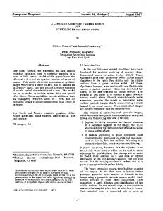
and thereby forming the tree. Further, in many cases, we would like to link an elastic rod to itself, thereby forming a ring. These rings could be further combined to large networks with complex topologies, as illustrated in Fig. 1. In this paper, we propose the Cosserat nets, a novel deformation model for the simulation of networks of elastic rods. The struts in the networks are simulated as elastic rods. We then propose a methodology to model the elastic joints. These joints have a given resting configuration. If the adjacent struts are rotated relatively to each other, then bending and twisting moments restore the reference shape. Our representation comes without additional constraint equations, and allows for an efficient local solution. In order to derive the necessary set of equations, we first discuss the deformation model C O R D E for the elastic rods that form the struts. The deformation model is based on [7]. In contrast to [7], an improved way to time-integrate the quaternions is proposed. This time-integration allows to neglect the inertia tensor since the time-integration is carried out in the local frame of each quaternion. Further, the benefits and limitations of the deformation model are thoroughly discussed. Moreover, we provide an extensive analysis of the trade-offs that have been accepted by the C O R D E model. To accomplish this, we present a constraint-free, fully dynamic reference deformation model. By comparing the static and dynamic behavior of C O R D E to this reference model, we quantify the approximation errors of C O R D E. Based on this investigation, we illustrate that C O R D E reproduces the non-linear mechanical effects that characterize elastic rods. Further, we show how to parameterize C O R D E such that the correct dynamics are plausibly approximated. Organization: After discussing the related work in Sec. II, we give a short introduction of the Cosserat representation of elastic rods in Sec. III. This should help the reader to get familiar with the terms and notation used in the paper. In Sec. IV, we describe the static simulation of elastic rods with C O R D E, which includes a discussion of the representation of the orientations. The extension to the dynamic case is detailed in Sec. V. Both sections include a comparison to the approach of [8]. The concept of Cosserat nets is introduced in Sec. VI. We evaluate our deformation model in Sec. VII. II. R ELATED WORK The Cosserat theory considers an oriented curve in space. The definition of a position and an orientation of the start and end point of the curve results in a boundary value problem (BVP). The analysis and numerical solution of the corresponding system of ordinary differential equations is discussed in, e. g., [9]. The analysis of the dynamics of inextensible rods is considered in, e. g., [10]. A comprehensive discussion of the topic is given in the book of Antman [11]. In computer graphics, we distinguish two different classes of approaches to simulate and animate elastic rods, namely approaches that consider the rod as a system of masses linked by springs, and approaches that consider the rod as a continuous curve in space. E. g. Chang et al. [12] proposed an approach


a)

b)

2

c)

d)

Fig. 1. Cosserat nets are graph-like structures that consist of elastic joints linked by elastic rods. In this paper, we propose to employ C O R D E to model such objects. Cosserat nets have a broad spectrum of applications in the field of animation. a) An animation of a chain modeled from linked elastic rings. b) Close-up of the chain. c) Animation of two heavy objects falling on two trusses. d) C O R D E is suited for simulating coarse nets.

that is focused on hair interactions, where the hair strand is modeled from clusters linked by bending springs. Brown et al. [1] published an approach to simulate knotting of ropes, including a robust collision handling scheme. They model the rope from a chain of masses and springs. However, in contrast to our deformation model, neither of these models is able to handle torsional torques. A deformable model that handles torsional torques has been presented by Wang et al. [13]. Similar to [1], they model a thread from a chain of springs. In addition, they link the segments by torsional springs. In contrast to their work, we employ an energy-based approach to compute the restoration forces. Choe et al. [14] proposed to model hair strands from rigid bodies linked by springs, where the torques are computed from the relative orientations of the rigid bodies. A similar model for the simulation of cables in virtual environments has been proposed in [15]. Recently, Hadap [16] describes a methodology based on differential algebraic equations to simulate chains of rigid bodies that includes torsional stiffness dynamics. In turn, this approach is computationally expensive and thus less suitable for interactive applications. The large stretching stiffness of elastic rods usually limits the efficiency. This problem is partially alleviated by Kubiak et al. [17] who combine the positionbased cloth-simulation approach of Mueller et al. [18] with a simple mass-spring approach to represent the rod. Similar in spirit is the approach of Selle et al. [19] that employs a concept they call ”altitude springs” to handle twisting deformation in the simulation of hair. For both approaches, material torsion is supported. However, since the twisting and bending moments are not coupled, many torsional effects cannot be reproduced. Terzopoulos [2] has been the first who considered a continuous energy formulation of the curve in space subject to geometric deformation. Later, Qin and Terzopoulos [20] proposed a physically-based deformation model of a NURBS curve. They derive continuous kinetic and deformation energies, and evolve the curve by employing Lagrangian mechanics. A finite element analysis enables the simulation of the curve at interactive rates. Similar in spirit is the approach of Remion et al. [21]. They employ successions of spline segments to model knitted cloth. In contrast to [20], they consider the control points as the degrees of freedom of the continuous object. The use of splines was also suggested by Lenoir et al. [3] and by Phillips et al. [22] in order to model threads. These approaches can also handle complex collision configurations, as recently shown by Kaldor et al. [23] in the context of the simulation of knitted cloth. Here, the authors model the yarn with one single spline, which is in contrast to [21]. These approaches have in common that material torsion can not

be represented. In contrast, our deformable model handles both bending and torsion of rods in contact. The Cosserat theory for elastic rods has first been introduced to the community by Pai in 2002 [6]. He models the statics of thin deformable structures such as catheters or sutures. He assumes the rod to be unshearable and inextensible. The configuration of the rod is obtained by solving the resulting BVP. This approach provides an efficient and physically correct way to animate continuous elastic rods. However, the model does not handle dynamics. Furthermore, self-contact and interactions require numerically sensitive shooting techniques to solve the differential equations. Recently, Bertails et al. [24] proposed an important extension of Pai’s work. They simulate hair strands as chains of helical segments. The Darboux vectors constitute the DOFs of the strand. To evolve the hair strands, they employ Lagrangian dynamics. The configuration of the hair strand is reconstructed from the generalized coordinates that conform to twist and curvature of the segments. Still, as their approach has complexity O(N 2 ) with N the number of segments, the approach is less suitable for handling contacts that require a large number of DOFs. In contrast, our scheme is linear in the number of elements, and designed to handle complex contact configurations such as knots. Further, we replace the viscous dissipation energy of [24] by a term that additionally considers internal friction without affecting the rigid body motion of the rod. Similar in spirit is the approach earlier proposed by Wakamatsu et al. [25] in the field of robotics. In contrast to Bertails et al., they employ the three Eulerian angles together with a stretch parameter as DOFs of the rod. The geometric configuration of the rod is then reconstructed by integrating the orientation field. However, it is unclear how the singularities of the Eulerian angles at the poles are handled. Moreover, the proposed model is limited to static equilibria. It is obvious to combine spline-based methods with the Cosserat approach. Theetten et al. proposed a geometrically exact, dynamic spline model which supports both geometric and material torsion [8], [26]. In contrast to Bertails and similar to us, they employ the spline control points as DOFs of the rod. Material torsion is modeled by a single roll parameter. This model is accurate, efficient, constraint-free and does not exhibit the ’ghost inertia’ problem of C O R D E (see Sec. V). However, a concept of material orientation cannot be easily handled with this formulation, as laid out in Sec. III. Moreover, their dynamic formulation is as well an approximation of the exact dynamics, as detailed in Sec. V. The research on elastic rods cumulates with a recent publication


of Bergou et al. which has considered the dynamic evolution of discrete elastic rods with torsion [27]. To represent the material torsion, they observe that the velocity of the twist waves is much larger than the velocity of the bending waves. Consequently, they do not carry the material torsion for each centerline segment. Instead, they represent the material torsion only at the boundary segments. To compute the variation in the material frames, they consider the discrete holonomy. The approaches that are most closely related to ours are the works of Grégoire et al. [28] and Loock et al. [29]. They proposed to model a cable from joined elements where each element has a position and an orientation, the latter expressed in terms of quaternions. Then they derive constraint energies and associated forces. The goal is to find static equilibria states of cables in virtual assembly simulation. We augment their work by considering the dynamics of rods, which provides unique challenges. Further, we employ finite element methods to derive discrete energies while they simulate the rod as a simple massspring system. III. C OSSERAT THEORY OF ELASTIC RODS In this section, we give a brief introduction of the Cosserat theory of elastic rods. The goal is that the reader becomes acquainted with the concepts and the notation of the configuration of elastic rods. For more information, we refer to the book of Antman [11].

3

d1 (σ2 ) d1 (σ1 )

r(σ1)

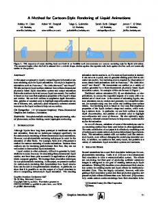
B. Representation An elastic rod can be thought as a long and thin deformable body. Since the volume of the rod is negligible compared to its length, we represent the centerline of the rod by a function r = r(σ) : [0, 1] → R3 that maps a line parameter σ to a position in the space. If we consider r to be a C 3 -differentiable function, we can derive expressions for the bending and geometric torsion by employing differential geometry. The geometric torsion measures the deviance of r from lying in a plane. E. g. a circle in space has zero torsion and constant curvature. However, with r alone, we cannot represent the material torsion, i. e. the ”roll” of the cross section around the centerline. Thus we have to introduce the concept of oriented curves: In each σ , we think of an orthonormal basis dk , k = 1, 2, 3 where the dk are called directors. We say that the directors are adapted to the curve, that means that the third director d3 (σ) is always parallel to the tangent r0 (σ) of the curve (see Fig. 2). The first and second directors d1 and d2 then indicate the orientation of the centerline. We thus denote the basis dk as the material frame of the rod. The directors dk (σ) constitute the columns of a rotation matrix R(σ) ∈ R3×3 , i. e. R = (d1 d2 d3 ). The parametrization of the rotation matrix (i. e. how to obtain the directors) is discussed in Sec. 4. To establish the stress-strain relation, we have to introduce a quantity that measures the rate of change in the position and orientation when traveling along the rod centerline. The rate

r(σ2)

d3 (σ1 ) d3 (σ2 )

d2 (σ1 )

Fig. 2. The configuration of the rod is defined by its centerline r(σ). Further, the orientation of each mass point of the rod is represented by an orthonormal basis, called the directors. d3 (σ) is constrained to be parallel to r0 (σ)

of change in the position of the centerline is a strain vector v = (v1 v2 v3 )T . As common in the treatment of elastic rods, shearing is neglected, thus v1 = v2 = 0. v3 is the stretch along the centerline, and it is measured as v3 = kr0 k

(1)

Without loss of generality, we assume the length of the unstretched rod to be 1. Consequently, v3 = 1 for the unstretched rod. Obtaining the orientational rate of change is slightly more involved. In differential geometry, this quantity is called the Darboux vector. It is a vector u0 ∈ R3 , and it is assembled from the areas that are swept by the directors when proceeding from σ to σ + ∆σ :

A. Notation Throughout this paper, scalar values are written in italic face (e. g. s), and vector values in bold face (e. g. s). If s(σ, t) is a function depending on the line parameter σ as well as the time ∂s(σ,t) t, then s0 (σ, t) denotes the spatial derivative ∂σ , and s(σ, ˙ t) ∂s(σ,t) denotes the temporal derivative ∂t .

d2 (σ2 )

u0 (σ)

=

=

3 X

lim

∆σ→0

k=1 3 X

1 2

dk (σ) × dk (σ + ∆σ) 2∆σ

(2)

dk (σ) × d0k (σ)

(3)

k=1

The Darboux vector measures the change of orientation in the reference frame. To relate the Darboux vector to bending and twist, we have to rotate it into the local frame (see Fig. 3), u = RT u0

(4)

or, written in terms of the directors dk , uk = dk · u0 ,

(5)

k = 1, 2, 3

T

with u = (u1 u2 u3 ) . When dealing with the dynamic case, j

u0 d3

RT

u

d2

d1

d1 d2

i

d3

u2 u3

u1

k

Fig. 3. To obtain the quantities uk , k = 1, 2, 3 related to bending and torsional strain, we rotate the Darboux vector u0 into the local frame, which is accomplished by multiplying u0 with RT .

quantities like velocity and angular velocity will come into play. ˙ The temporal derivative r(σ) of the centerline at σ denotes the translational velocity of the centerline. The angular velocity ωk of the directors around the k-th axis is obtained likewise as ωk = dk · ω0

(6)


with

3 1X ω0 = dk × d˙ k 2

4

(7)

k=1

C. Constitutive relations To study the static equilibria of elastic rods, we have to find a stress-strain relationship. To accomplish this, we define a scalarˆ ) with a minimum valued, convex energy function V (v3 − 1, u − u ˆ = (ˆ at (0, 0). Here, u u1 u ˆ2 u ˆ3 )T corresponds to the intrinsic bending and torsion of the rod and allows to model e. g. spirals, as illustrated in Fig. 4. The stresses (i. e. the restitution forces) are then obtained by differentiating the energy with respect to the coordinates.

Fig. 4. An elastic spiral is subject to continued torsional load. This load makes the spiral twisting around itself in order to balance the twisting and ˆ > 0. bending strains. The spiral is an elastic rod with an intrinsic curvature u

bend? The answer is that it will stay in the straight configuration: it is in an unstable equilibrium. As soon as the centerline is slightly disturbed, it will immediately pop out, striving towards a stable equilibrium between the torsion, bending and stretching strains (Fig. 5, bottom). This experiment provides a simple way to evaluate the plausibility of an (extensible) elastic rod deformation model. In Sec. VII, we show that the C O R D E model exhibits this behavior. In contrast, approaches that do not treat bending and torsion in a unified manner such as [17] cannot reproduce this behavior.

Fig. 5. A perfectly straight rod that is subject to a torsional load is in an unstable equilibrium (top). As soon as the centerline is slightly disturbed, the rod starts to bend until an equilibrium between torsion, bending and stretching strain is reached (bottom). Approaches that do not treat bending and torsion in a unified manner cannot reproduce this behavior. This experiment provides a simple way to verify the physical plausibility of an elastic rod deformation model.

V = Vs + Vb is the sum of a (translational) stretch energy Vs and a bending energy Vb . We define the stretch energy Vs to be a quadratic form in the stretch v3 Vs =

1 2

Z

1

0

Ks (v3 − 1)2 dσ

(8)

Ks is the stretching stiffness constant that is computed from a stretching Young’s modulus Es and the radius r with Ks = Es πr2 . Likewise, the bending energy Vb is a quadratic form in the strain rate vector u, Z 1 1 ˆ ) · K(u − u ˆ )dσ Vb = (u − u (9) 2 0

The matrix K = (Kkk ) ∈ R3×3 is the stiffness tensor. If we assume that the rod is a solid body with the radius r small compared to its length, then (9) can be rewritten as Vb =

1 2

Z

1

3 X

0 k=1

with K1 = K2 = E

Kk (uk − u ˆk )2 dσ

πr 2 , 4

K3 = G

πr 2 2

(10)

IV. T HE C O R D E MODEL In the previous section, we have stated the continuous deformation energies that are functions of the strain rates. In this section, we propose a discretization of the rod into control points. This part comes with a discussion on the representation of the rotation. We then derive the formulations for the deformation energies per element by employing finite element methods.

A. Discretization We discretize the centerline of the rod into N spatial control points ri ∈ R3 , i ∈ [1, N ]. Thus we have N − 1 centerline segments. To represent the orientations of these centerline segments, we additionally employ N − 1 material frames Rj ∈ R3×3 , j ∈ [1, N − 1], as illustrated in Fig. 6. In the subsequent subsection, we show how to parameterize the rotation matrices. By dk (Rj ), we denote the k-th director of the j -th material frame, which is obtained as the k-th column of the rotation matrix Rj .

(11)

with E denoting the Young’s modulus governing the bending resistance, G denoting the shear modulus governing the torsional resistance, and r denoting the radius of the rod’s cross section. Details are found in [9]. At this point, it is worth making a note on the balance of the strain rates. By minimizing V , the strain rates uk and v3 are balanced. Thus if an elastic rod suffers from torsional strain, then this strain will balance, resulting in a bending deformation. This coupling between the strain rates is responsible for the looping phenomenon of elastic rods under torsional strain (see Fig. 4). Now consider a perfectly straight rod that is subject to torsional load (Fig. 5, top). In which direction does it start to

ri+2

Rj+1

Rj+2

ri Rj ri+3 ri+1

Fig. 6. The centerline of the rod is discretized into nodes ri . We additionally consider N − 1 material frames Rj to express the orientation of the center segments.


5

The spatial derivative r0i of the centerline is related to the stretch of the centerline. Thus to compute r0i , we employ a simple springbased formulation, namely r0i =

1 (ri+1 − ri ) li

(12)

where li = kr0i+1 − r0i k is the resting length. Thus, in the unstretched case, v3 = kr0i k = 1 as demanded. B. Parametrization of the rotation matrix In this subsection, we discuss the representation of the material frames Rj . From the material frames, we can in turn compute the Darboux vectors that are related to the bending and twisting strains. From a theoretic point of view, it is possible to reconstruct Rj from the centerline segment (ri , ri+1 ) and a single roll parameter ϕi ∈ R. However, this cannot be done without considering the temporal coherence. A simple setup (Fig. 7) illustrates this problem: Consider an elastic rod whose left end point stays fixed. The first director d1 initially points towards the positive y-axis. If this rod is rotated around the z-axis, then we would intuitively end up in the first director d1 pointing towards the negative y-axis. If, in contrast, this rod is rotated around the y-axis, then the first director should intuitively keep pointing upwards. Still, in both cases, the rod has not been subject to any roll torques, thus ϕ will not have changed its value. As a consequence, the material frames cannot be computed unambiguously. Even worse, considering that the segment orientations in a deformed rod might cover the whole space SO(3), a globally coherent material direction cannot be computed. y

y d1

x

d1

z

contrast to other SO(3) representations such as Euler angles, they provide a singularity-free parametrization of Rj . The conceptual advantage of this approach is that since the material frames of the rod are now fully determined by the quaternions, we can compute the bending and twisting moments without considering the control points ri . The resulting torques accelerate the quaternions towards an energy-minimizing configuration. As a consequence, the material direction (which is given by the quaternions) is always globally coherent. In turn, this enables a straight-forward derivation of internal friction forces. C. On quaternions We consider a quaternion q to be a vector q = (q1 , q2 , q3 , q4 )T ∈ R4 with qk = ak sin(θ/2), k = 1, 2, 3, and q4 = cos(θ/2). Here, (a1 a2 a3 )T is the rotation axis, and θ is the rotation angle. Since only unit quaternions represent pure rotations, the four parameters qk are coupled by the constraint q12 + q22 + q32 + q42 = 1. The rotation matrix R is parameterized by 

q12 − q22 − q32 + q42  2(q1 q2 + q3 q4 ) 2(q1 q3 − q2 q4 )

R= 2(q1 q2 − q3 q4 ) −q12 + q22 − q32 + q42 2(q2 q3 + q1 q4 )

We approximate the spatial derivative q0j as q0j =

1 (qj+1 − qj ) lj

Fig. 7. It is not possible to compute an unambiguous material direction without considering the temporal course of the simulation. In both scenarios, the rod has not been subject to any rolling during the rotation, still, the material directions of the target states differ.

There do not exist straight-forward solutions to circumvent this problem. An approach that considers infinitesimal transformations has been proposed by Boyer et al [30]. Up to now, the approach in [8] is the only one in the field of computer graphics that employs the control points along with a roll angle as DOFs. Their approach has the advantage that the computation of the strain rates does not rely on globally coherent directors. Instead, they compute the strain rates as the sum of the geometric torsion and the spatial change of material torsion. However, in order to visualize the rods, they need to update the material frames. They propose to update the first frame of the rod by employing temporal coherence, and then to propagate the material frames along the rod. In contrast, we propose a different approach that avoids the problem of explicitly updating the material frames in a natural way: Instead of reconstructing the frames from a roll angle, we express the material frames by quaternions qj , j ∈ [1, N − 1]. In

(13)

By considering that the quaternions ’sit’ on the midpoints of the centerline segments, we approximate the step length lj of the quaternion forward difference as lj = 21 (kr0i+2 − r0i+1 k + kr0i+1 − r0i k). Computing the spatial derivative d0k (qj ) is more involved (see Appendix I). The strain rates uk governing the constitutive relations can be computed as uk = 2Bk q · q0 ,

z

 2(q1 q3 + q2 q4 )  2(q2 q3 − q1 q4 ) −q12 − q22 + q32 + q42

k = 1, 2, 3

(14)

where the Bk ∈ R4×4 are constant skew-symmetric matrices. The derivation of (14) is given in the Appendix. Up to now, we have treated the centerline ri and the orientations qj as separated entities. However, in contrast to the rigid body simulation, the positions and the orientations cannot be simulated independently. Instead, the material frames parameterized by qj and the control points ri are coupled by the constraint that the third director d3 (qj ) is parallel to the tangent r0i , i. e. r0i − d3 (qj ) = 0 kr0i k

(15)

In the past, several approaches have been proposed to handle constrained mechanical systems, e. g. by employing Lagrangian multipliers or reduced coordinates. For the sake of efficiency and simplicity, we employ the penalty method which has the further advantage that the constraints can be handled locally. We thus model the holonomic constraint (15) by a convex energy function Ep [i]

= =

Z ´ ³ r0 ´ 1 li ³ r0i i − d3 (qi ) · − d3 (qi ) dξ (16) κ 0 0 2 0 kri k kri k ´ ³ r ´ li ³ ri+1 − ri i+1 − ri κ − d3 (qi ) · − d3 (qi ) 2 kri+1 − ri k kri+1 − ri k

By differentiating this penalty energy with respect to the coordinates ri and qj , we obtain penalty forces that maintain the constraints. κ is a spring constant that should be in the same


6

order as Ks . We treat the penalty energy as an additional potential energy term. If the method of Lagrange multipliers is employed, the introduced stiffness could (at least partially) be removed. However, we would end up in solving a banded linear system, whose inversion is in turn less efficient. Moreover, it does not solve the ’ghost inertia’ problem related to the dynamic case that is discussed in the subsequent section. To enforce the quaternion unit constraint kqj k = 1, we employ the simple method of coordinate projection, i. e. we normalize the quaternions in each simulation step. Although this procedure does not conserve the energy, experiments indicate that it is a good compromise between efficiency and accuracy. D. Finite element model In the previous sections, we have discretized the rod into disjoint centerline elements i = (ri , ri+1 ) and disjoint orientation elements j = (qj , qj+1 ). The DOFs of the rod are constituted by the 3N + 4(N − 1) DOFs of these control points and quaternions. A finite element (FE) method usually solves the weak form of the static stress analysis for kinematically admissible coordinates ri and qj , ˆ) − V (v3 − 1, u − u

N X

ri · fie dσ = 0

that satisfy the given boundary conditions. fie are the external forces acting on the points, external torques are neglected. Having in mind that we finally want to solve the dynamic equilibrium of the rod, we do not discuss the static solution further. Instead, we [i] employ the FE method to compute the restitution forces ∂V ∂ri and [j] torques ∂V ∂qj per element. These forces and torques accelerate the elastic rod towards the static equilibrium. The goal now is to derive the potential energy V [i] and V [j] per centerline element i and orientation element j , respectively. By differentiating these energies with respect to the local coordinates, we obtain the forces and torques acting on the control points and material frames. To compute the per-element potential energy, we have to interpolate the unknown displacement field within the elements. For simplicity, we employ piecewise linear shape functions that interpolate the coordinates ri and qj linearly and result in constant stretch- and strain rates within the elements. They result in particularly simple expressions when integrated over the element length. Experiments indicated that higher-order shape functions do barely increase the accuracy of the model. We further employ constant shape functions to interpolate the spatial derivatives r0i and q0j , i. e. they are assumed to be constant within the elements. The stretch energy Vs [i] per centerline element i is obtained by integrating the stretch over the element length li Z 1 li Ks (kr0i k − 1)2 dξ 2 0 q 1 1 l i Ks ( (ri+1 − ri ) · (ri+1 − ri ) − 1)2 (18) 2 li

= =

Likewise, the bending energy per orientation element j is obtained by integrating over the element length lj Vb [j]

=

=

1 2

Z

lj

0

3 X

– · q0 − uˆ )2 dξ Kk (2Bk q j k j

(19)

k=1

3 lj X 1 ˆk )2 Kk (Bk (qj + qj+1 ) · (qj+1 − qj ) − u 2 lj k=1

V. T HE DYNAMIC EVOLUTION In this section, we discuss the effects that come into play when the dynamic evolution of the rod is considered. We first show how to obtain the simplified rod dynamics that avoid the solution of a system of equations. We then propose a way to compute internal friction forces that plausibly damp relative motion within the rod. Last, we discuss the artifacts that are caused by the approximative dynamic C O R D E model, and show how to reduce those artifacts.

(17)

i=1

Vs [i]

By employing FE methods to compute the restitution forces, we ensure that the static equilibria are independent from the underlying discretization (at least as long as the DOFs of the rod suffice to reproduce the deformation). This property is particularly interesting in the context of adaptive simulations, as pointed out in [31]. Summarizing, we have now computed the potential energy per element. By symbolically differentiating the sum V [i] = Vs [i] + Ep [i] with respect to ri and ri+1 , and by differentiating the sum V [j] = Vb [j] + Ep [j] with respect to qj and qj+1 , we obtain the restitution forces and torques acting on ri , ri+1 , qj and qj+1 . In the next section, we describe how we compute the trajectories of the control points and quaternions that are governed by the restitution forces.

A. Numerical time-integration The dynamic equilibrium of a mechanical system is usually obtained by feeding the Lagrange equation of motion, a variational formulation of the equations of motion. This results in a system of the form Ma − f = f e . When considering rotating mechanical systems, the mass-matrix M will be block-diagonal sparse or dense. In any case, inverting the mass-matrix requires the iterative solution of a system of equations which can be expensive. However, we can obtain an intrinsically simpler way to compute the dynamics by looking at the solution that we have presented in the previous section. We consider the rod as a chain of control points ri , and a chain of quaternions qj conforming to the material frames. These chains are loosely coupled by penalty forces that accelerate them towards a valid configuration. Still, the dynamic evolution of the mass points is decoupled from the dynamic evolution of the quaternions. As a consequence, we can time-integrate the control points as if they were mass-points in a mass-spring system, and the quaternions as if they represented the orientation of rigid bodies. We assume that the masses mi = 21 ρπr2 (li−1 + li ) are lumped in the control points ri . Here, ρ is the density of the rod, and r is its the radius. Then the numerical evolution of the mass points is governed by the equation of motion mi ¨ri − fi = f e , where fi is the sum of the internal forces on ri . To evolve the mass points, we employ a semi-implicit Euler scheme. For the evolution of the quaternions, we can stick to the wealth of literature on rigid body simulation. It is most common to express the angular velocities ωj ∈ R3 along with the quaternions qj as state variables [32]. We then obtain the state equations for the quaternions qj as ω˙ j

=

q˙ j

=

I−1 (˜ τj − ωj × Iωj ) µ ¶ ωj 1 Q 2 j 0

(20)

Here, Qj is the quaternion matrix that allows to write the quaternion multiplication consistently as a matrix-vector multiplication. Further, τ˜j ∈ R3 are the internal torques that govern


7

the restitution. We have to consider that the torques τj ∈ R4 b [j] that result from evaluating ∂V are dual to the quaternions. ∂qj The translation into the spatial torques τ˜j is accomplished by a multiplication with the transposed quaternion matrix QTj , µ

¶

τ˜j 0

1 T Q τj 2 j

=

(21)

Details can be found in [32]. I ∈ R3×3 is the inertia tensor of the rod segment. For rods, we assume it to be a diagonal matrix I = (Ikk ), k = 1, 2, 3 with I11 = I22 = 14 ρπr2 and I33 = I11 + I22 . For diagonal matrices, the coriolis force term ωj × Iωj = 0. Thus we obtain the simple quaternion state equations µ

ω˙ j 0

¶ =

1 −1 T Qj τj 2I

µ q˙ j

=

1 2 Qj

ωj 0

¶

(22)

that are numerically integrated with a semi-implicit Euler scheme. B. Modeling internal friction In order to plausibly model elastic rods, the internal friction has to be considered. Internal friction forces damp relative motion in the rod. As Baraff et al. [33] pointed out, friction forces that reduce stretch oscillations should confine itself solely to relative stretch motions, and not to any other relative motions. The same criterion applies for angular friction forces. We thus define a translational dissipation energy per element i Dt [i] =

1 2

Z

li

(rel)

γt vi

0

(rel)

· vi

dξ =

li (rel) (rel) γt vi · vi 2

(23)

where γt is the translational friction coefficient. Moreover, v(rel) is the relative velocity of the two control points constituting the centerline element, projected on the tangent r0 of the centerline, (rel)

vi

1 r0 (r˙ 0 · r0 ) kr0i k2 i i i | {z }

=

≈1

³ ´ ˙ ˙ (r − r ) ( r − r ) · (r − r ) (24) i+1 i i+1 i i+1 i 3

1

=

li

where we made the simplifying assumption that kr0i k ≈ 1, which is valid for rods with a large stretching stiffness. The angular dissipation energy derives from the spatial derivative ω 0r of the angular velocity ω r . Here, ω r = (ω1r ω2r ω3r )T is the angular velocity of the material frames expressed in the reference frame that is computed as ˙ q) = 2B0k q · q˙ ωkr (q,

(25)

It is important to consider the angular velocities in the reference frame since quantities cannot be compared in different local frames. We then obtain the angular dissipation energy per orientation element j as Dr [j]

= =

=

1 2 1 2

Z Z

lj 0

γr ω 0r (q˙ j , qj ) · ω 0r (q˙ j , qj )

3 X 1 1 ( 2B0k qj+1 q˙ j+1 − 2B0k qj q˙ j )2 dξ lj lj

lj 0

2 γr lj

(26)

γr

k=1 3 X

(B0k qj+1 q˙ j+1 − B0k qj q˙ j )2

k=1

(27)

A similar dissipation energy formulation is proposed in [25]. The damping forces are now derived by symbolically differentiating the dissipation energies with respect to the coordinates. We employ Maple v9.51 to carry out the calculations. This relatively straight-forward derivation of internal friction is enabled since the quaternions allow us to symbolically express the material direction and the angular velocity of the material in a globally coherent manner. This is in contrast to the approach of [8] that does not symbolically derive a globally coherent material direction. Thus the computation of angular friction is intrinsically more difficult. Consequently, they do not model internal friction but employ the viscous friction that is a side-effect of their implicit solver. C. Benefits, limitations and future work The proposed approach computes the dynamic evolution of the rod as a loosely coupled motion of a chain of masses and a chain of quaternions. The explicit simulation of the quaternions enables a convenient computation of the material direction, which allows a direct solve of the equations of motion, resulting in a comparably small implementation effort. Further, a consistent explicit representation of the material direction simplifies the computation of internal friction and also eases a texture-mapped visualization of the rod. However, the proposed approach comes with an artifact we denote as ’ghost inertia’. Consider a simple pendulum that conforms to an elastic rod whose one end is fixed, and whose other end is being elongated. By swinging around the vertical equilibrium position, the rod is subject to a rigid body rotation. Still, the material frames need to evolve continuously in order to adapt to the continuously changing orientation of the rod centerline. This evolution is solely governed by the parallel-constraint (16). The noticeable behavior is that the rod movement is subject to a rotational drag, i. e. a ghost inertia. This rotational drag increases with increasing weight of the material frames. The ghost drag is only noticeable if the rod is subject to rigid body rotation modes. To overcome this problem, we reconsider our primary goal, namely that the bending inertia of the rod is exclusively governed by the centerline while the torsion inertia is governed by the quaternions. This conforms to an inertia tensor I with I11 = I22 = 0. Obviously this inertia tensor is singular. However, by scaling I11 and I22 with a factor α < 1, we get a DOF that controls the amount of ghost inertia we are willing to accept: By choosing a small α < 10−2 , the ghost inertia is hardly noticeable, but the numerical integration requires a smaller time step due to the increased stiffness, which can in turn remedied with time substepping for the quaternion integration. The time step hq for the quaternion integration depends on the simulation setting. In many cases, α = 10−2 provides a fair compromise between ghost inertia and efficiency. We finish this section with a short summary on the rod dynamics in previous approaches, and an outlook to future work. Most previous approaches compute a static or a quasi-static equilibrium configuration [6], [25] and thus do not consider dynamic effects. Bergou et al. propose to consider the centerline as dynamic while treating the material torsion as quasi-static, which is a fair approximation if small rod radii are considered [27]. The dynamic approaches of Bertails et al. [24] and Chang et al. [12] have in common that the DOFs of the model are provided by the strain rates uk and v3 . They then reconstruct 1 www.maplesoft.com


the centerline, given the position of the first node of the rod. Both approaches propose to derive the dynamics with the Lagrangian formalism, and both approaches give R L the kinetic energy governing the dynamic evolution as T = 0 ρAr˙ 2 dσ . However, thereby, both approaches neglect the angular momentum of the rod crosssection. R LTheetten et al [8] approximates the kinetic energy as T = 0 (ρAr˙ 2 + I33 θ˙2 )dσ , where θ is the roll of the material cross-section. Thus this formulation considers the inertia of the torsion. Still, they neglect the bending and twisting moments of the angular cross-section. In contrast,R the correct kinetic energy is L e. g. given by Antman [11] as T = 0 (ρAr˙ 2 + ω · Iω)dσ , where the second term conforms to the rotational kinetic energy of the rod cross-section. It is not easy to quantify the error in the discrete case that is introduced by neglecting the rotational kinetic energy. To seek for an analogy, computing the kinetic energy of a discretized rigid body by summing the translational energies of the nodes provides but an approximation of the rotational energy. In order to quantify the approximation of our model, we have implemented a Cosserat rod element model recently proposed by Cao et al [5] that considers the exact kinetic energy (see Appendix II). We give the results of this comparison in Sec. VII. However, we underline that there is still room for improvement in terms of simulating the dynamics of elastic rods in an accurate and efficient way. VI. C OSSERAT NETS In this section, we describe a novel extension of the previously described approach to branched and looped structures. The motivation comes from the observation that the C O R D E model basically computes per-element forces on control points and orientations. The resulting restitution forces on the control points and material frames result from the contributions of the adjacent elements. Thus it is obvious that the last and the first control point of a rod could be merged, thereby forming a closed loop. Moreover, instead of restricting a control point to be adjacent to two centerline elements, we could allow T-junctions, i. e. that the rod branches in a control point. A. Theoretical background We define a Cosserat net to be a set of elastic joints, linked by elastic rods. The joints are elastic in the sense that the linked elastic rods are allowed to bend and twist relative to each other. The constitutive restitution is governed by given elasticity moduli. Intuitively, we demand that the static equilibrium of e. g. a Tjunction with one 180◦ and two 90◦ angles should conform to the static equilibria of rods with intrinsic curvatures of 180◦ and 90◦ , respectively. Branched elastic rods have rarely been considered in the literature. In [34], Nadler and Rubin have proposed to model threedimensional frames from elastic beams joined by Cosserat points. A Cosserat point can be understood as a deformable cuboid, where the deformation modii are decoupled into homogenous and into inhomogenous deformations. More information on the theory of Cosserat points can be found in [35]. In computer graphics, branched elastic structures such as trees have mainly been considered in the context of articulated rigid bodies, see e. g. Hadap [16] or Weinstein et al. [36]. Other works have focused on the modal analysis of the dynamics of treelike objects [37]. However, these formulations do not consider torsional deformation of the joints, which is in contrast to our approach.

8

B. Our approach We propose an intuitive approach to model these networks of elastic rods and elastic joints. In contrast to [34], the focus is on the plausible and efficient animation of such networks. We first demand that joints always coincide with control points of the discretized rods. This can be start points, end points, or arbitrary control points within the rod. Notice that this does not limit the generality of the approach because control points can be adaptively inserted without making the global deformation behavior change, as illustrated in our previous work [31]. We then assemble the Cosserat net from single elastic rods that share one or more control points. The stretch forces and the penalty forces for the parallelconstraint are computed by integration over the centerline elements. Consequently, we can compute these forces in all centerline elements of the network. The restitution forces on the control points are obtained by summing the contributions of all adjacent elements. It is easy to verify that the proposed discretization of the domain of the Cosserat net is disjoint, thus the computation of the stretch and penalty forces is physically plausible (see Fig. 8 left). Things become more difficult if we consider the bending forces, because these forces are computed by integration over the orientation elements that link two centerline elements (see Fig. 8 right). However, we cannot discretize a T-junction into disjoint orientation elements, as depicted in Fig. 8. We could, of course, omit the orientation elements in the T-junctions, but this would result in a joint that does not restore its resting configuration after deformation, which is not what we want. Instead, we propose a concept that is a straight-forward extension of the case of one-dimensional rods. In a joint, we consider all pairs of adjacent centerline segments, and treat these pairs as orientation elements. E. g. for a T-junction, we end up in having three orientation elements (Fig. 8 right), and for a star n with n adjacent segments, we obtain ( 2 ) orientation elements. Further, these orientation elements have a discontinuous, intrinsic curvature that conforms to the resting angle between the adjacent segments. To compute the restitution torques in a joint, we now integrate over all orientation elements and sum the torques per orientation node. While this concept lacks some physical accuracy, it meets the requirements in animation: an easy and fast solution that reproduces the behavior that we intuitively expect. Still, future work includes a more accurate handling of these joints. ri+4 qj+3

ri+1

ri+2

ri+3

qj+1

qj+2

qj ri

Fig. 8. Left: A T-junction always conforms to a control point of the discretized rods. A Cosserat net is then assembled from the single elastic rods that share control points. Right: We consider all pairs of adjacent segments as orientation elements, depicted as dashed lines. Thus, for a T-junction, we end up with the three orientation elements (qj , qj+1 ), (qj , qj+3 ) and (qj+1 , qj+3 ) modeling the joint.


9

VII. E VALUATION AND APPLICATION

We have proposed to model the elastic rod from control points that define the configuration of the centerline, and from quaternions that define the material frames. The twisting and bending moments are computed by minimizing the respective energies. In turn, the twisting and bending energy results from the squared Darboux vector. Thus, by minimizing the Darboux vector, we automatically couple the twisting and bending moments. Thereby, we win physical plausibility and can reproduce the interesting buckling and looping phenomena subject to elastic rods. To illustrate this property of the C O R D E model, we perform the experiment that we have already sketched in Sec. III. We consider two elastic rods, one is simulated with C O R D E, the other with the reference model. Both rods have a Young modulus E = 1MPa, a shearing modulus G = 4MPa, a stretching modulus Es = 1GPa, a radius r = 0.01m, a density ρ = 1300kg m−3 and length 10m. Since internal friction has not been implemented for the reference model, we are employing viscous friction in this experiment. Further, the penalty constant for the C O R D E rod is κ = 106 kg m s−2 , and time step of the simulation is 10−4 s. We span the two perfectly straight elastic rods between two anchors and twist the material frames around the centerlines such that the end-to-end rotation angle is 32 π . The rods are now in an unstable equilibrium. As long as the centerlines stay straight, the unstable equilibria are held. As soon as the centerlines are slightly disturbed, the rods start to buckle until stretch, bending and torsional strain are balanced. In Fig. 9, we see the comparison of the two deformation models in the unstable equilibrium (left) and after having reached a stable equilibrium that balances between the stretch and strain rates (right). The resting state of the C O R D E model is less curved than the resting state of the reference model. The reason for this asymmetry is the constraint energy that absorbs some of the total potential energy. The temporal course of the simulation is illustrated in Fig. 10. We plot the strain energy of the four deformation modes (first bending, second bending, torsion and stretch) plus the sum of those energies. The goal of this experiment is to illustrate the qualitative buckling behavior of C O R D E. In the beginning, both rods are in the unstable equilibrium and the total energies conforms to the torsion energies. If there were no external forces acting on

the centerlines, they would keep the unstable equilibrium. Thus, in order to induce the buckling, we exert a small gravitational force on the centerlines. The rods immediately pop out, striving towards stable equilibria states that balance between the four deformation modes. This is indicated in the total energies that have decreased after the rods found their equilibria. In contrast, the bending and stretching energies have increased, indicating that the centerlines are no longer straight. While the reference model accurately balances between stretch and bending modes, the C O R D E deformation model has a much lower stretch energy. This comes from the penalty method that absorbs some energy. Moreover, the two sets of curves differ in terms of the decay of the oscillations, which is due to the fact that our implementation of the reference model does not support internal friction but only viscous damping. Still, we conclude that C O R D E reproduces the buckling behavior which illustrates the physical plausibility of the proposed deformation model. Torsion simulation with CoRdE

1st bending 2nd bending Torsion

Strain energy

A. Evaluation of the static behavior

Fig. 9. Two elastic rods under torsional load are in an unstable equilibrium (left). If the centerline is disturbed, then the rods buckle in order to balance bending, torsion and stretch strains. The upper rod is simulated with C O R D E, the lower rod with the reference model. The penalty method of C O R D E absorbs energy, thus its resting state is less curved than the resting state of the reference model.

Stretch Total

0

2000

4000

6000

8000

10000

Torsion simulation with reference model

Simulation step

1st bending 2nd bending Torsion

Strain energy

In this section, we give an extensive and careful evaluation of the proposed deformation model C O R D E. We focus on two aspects: First, we evaluate the C O R D E model with respect to both the static and the dynamic equilibrium. To accomplish this, we have implemented a reference deformation model that bases on previous work in the field of mechanics [5]. The reference model bases on the FE method, is constraint-free and computes the correct dynamics in the sense of Antman [11]. Details are found in the Appendix II. The expensive assembly of the mass matrix and the numerical instabilities around the poles make the reference model of little practical interest in computer graphics. However, by comparing C O R D E to the reference model, we can show how to parameterize C O R D E such that the artifacts introduced by the approximations are minimized. In a second part, we present examples that illustrate the wide applicability of Cosserat nets. In the experiments, the collision handling has been carried out with the approach presented in [31]. All experiments have been performed on an Intel Xeon PC with 3.8GHz.

Stretch Total

0

2000

4000

6000

8000

10000

Simulation step

Fig. 10. Temporal course of the torsion experiment. The goal of this experiment is to illustrate that by minimizing the Darboux vector, C O R D E reproduces the buckling behavior, which underlines the physical plausibility of the deformation model. In fact, both deformation models reproduce the buckling behavior that exhibits in the sudden increase of the bending and stretch energy. The total deformation energy, however, has decreased after the buckling, indicating that the rods have reached a stable equilibrium. The reference model balances accurately between bending and stretch.

B. Evaluation of the dynamic behavior As illustrated in Sec. V, the C O R D E model simulates the elastic rod as a chain of mass points and a chain of quaternions. The coupling is realized with the penalty method. If now a rod is subject to a rigid body rotation, then we account twice for the moment of inertia, once by accelerating the centerline, and once


Elongation [m]

Elongation [m]

Elongation [m]

Elongation [m]

by accelerating the quaternions. This results in a visible drag or ’ghost inertia’. We proposed to overcome this limitation by scaling the first two diagonal entries of the inertia tensor (that conform to the bending moments of the quaternions) by a factor α < 1. The smaller the α-parameter, the better we approximate the optimal solution, which conforms to quaternions that have only a moment of inertia when rotated around the third axis (conforming to torsion). To illustrate this problem, we perform an experiment of a simple elastic pendulum: We attach the upper end of two vertically hanging elastic rods, and elongate the lower ends (the elastic rods have the same physical properties as in the experiment described above, except for internal damping which is γt = γr = 0). One rod is simulated with C O R D E, the other with the reference deformation model. The time step of the simulation is 10−4 s. Upon releasing the lower ends, the elastic rods swing about their vertical equilibria. In this setting, the rods are subject to rigid body rotations, thus the C O R D E rod reveals the ’ghost inertia’ phenomenon. We simulate the C O R D E rod with α = 1, α = 10−1 , α = 10−2 and α = 10−3 . In Fig. 11, we plot the elongation of the elastic rods over time. As the graphs illustrate, the smaller the α-values (i. e. the ’lighter’ the quaternions), the better is the approximation of the dynamics of the C O R D E rod. The reference model does not reveal this artifact since its dynamics are exclusively governed by its 4N DOFs (see Appendix). Notice that smaller α-values require more accurate numerical integration schemes, thus choosing an α-value is always a trade-off between efficiency and accuracy. To account for smaller α-values, we timeintegrate the quaternions at a smaller time-step hq . This technique is sometimes referred to time sub-stepping. 0.4

α = 1.0

α = 0.1 Reference model CoRdE

0 -0.2

Time α = 0.01 Reference model

0.2

CoRdE

0 -0.2

Time α = 0.001 Reference model

0.2

CoRdE

0 -0.2 -0.4

−3

10 10−3 5 · 10−4 6.6 · 10−5 6.75 · 10−6

#sub-steps =

h hq

Time [ms]

1 1 2 15 148

0.21 0.21 0.39 2.86 28.23

Fig. 12. This table summarizes the maximum possible sub-step hq for different α-values, given a constant time step h. The last column shows the time that is needed to perform the time-integration of the whole net, including the computation of the elastic forces, the time-integration of the mass-points and the time sub-stepping of the quaternions. The time measurements indicate that the effort grows linearly with the number hh of sub-stepping iterations. q

is illustrated in Fig. 15 a). The ribbon is simulated as a Cosserat net, consisting of two elastic rods linked by struts, and it is discretized in 86 points and 127 quaternions. The mass points are integrated with a constant time step h = 10−3 s. We simulate the net with different α values ranging between α = 1 and α = 10−4 . For each α, we experimentally determine the maximum sub-step hq of the quaternion time-integration such that the simulation sequence can be simulated without crashing. The values for α and hq , and the time to perform the timeintegration of the whole net are summarized in Fig. 12. This time measurement includes the computation of the elastic forces, the integration of the mass points and the sub-stepping for the timeintegration of the quaternions. Since smaller sub-steps hq require more sub-stepping iterations – notably hhq , and since in each sub-stepping iteration, the bending and constraint forces must be re-computed, the time needed for the integration increase with decreasing sub-steps hq . C. Cosserat nets

Time

0.2

-0.4 0.4

1 10−1 10−2 10−3 10−4

Sub-step hq

CoRdE

0 -0.2

-0.4 0.4

α

Reference model

0.2

-0.4 0.4

10

Time

Fig. 11. Temporal courses of the pendulum experiment. The visual drag influences the frequency of the pendulum. The smaller the α values, the better is the approximation of the correct dynamics of the reference model. In turn, small α-values require a smaller step for the numerical time-integration, which is remedied with time sub-stepping.

It is not easy to establish an analytical relationship between the scalar α and the maximum sub-step hq for the numerical timeintegration of the quaternions that results in a stable simulation. That is because the stability of the simulation of a C O R D E rod depends on many parameters such as the internal and viscous damping and the magnitude of external forces arising in the simulation. Moreover, the amount of ghost inertia that is accepted during the simulation cannot be expressed in numbers but depends on the simulation and the observer. However, to give an idea about the stability and performance of the dynamic simulation with respect to α, we perform an experiment of a ribbon falling onto the ground, thereby colliding with itself and undergoing massive deformation. The experiment

The Cosserat nets are an important extension of the C O R D E deformation model to graph-like structures. The resulting networks of elastic rods linked by elastic joints allow to model a large variety of solids. To illustrate the wide applicability of the proposed deformation model, we have performed a series of experiments. We underline that the focus is more on the animation than on the mechanical simulation of the modeled objects. For all experiments, α = 0.02 and hq = h. In contrast to previous approaches [16], [36], our representation allows to compute both forces and torques on joined elements, based on the bending and torsional shearing between adjacent segments. To illustrate that the treatment of torsional deformation results in a different behavior that cannot be reproduced by handling bending deformation alone, we have staged an experiment where two elastic trusses are attached on the left side, but allowed to freely moving elsewhere. The trusses deform under the influence of gravity, as illustrated in Fig. 14. Both trusses have a Young modulus E = 200MPa, a stretching modulus Es = 2GPa, a radius r = 0.01m, and a density ρ = 1300kg m−3 . Their planar extends are 11 × 2 meters. Since we are interested in studying the static resting states, we do not model internal friction but employ external (viscous) damping. The blue truss in the back has a shearing modulus G = 200MPa, while the green truss in front has no resistance to torsional shearing. As Fig. 14 a) illustrates, the static resting configuration of the two trusses differs significantly. While the blue truss hangs stable with only mild deformation, the green truss is flexed. This apparently different behavior comes in fact from the reduced


11

Fig. 13. We vary the end-to-end rotation of a spheroidal object that consists of four elastic rods. This experiment illustrates the rich deformations that are achieved by employing C O R D E to model such networks of joints and elastic handles.

stability of the green truss that is induced by the non-existing torsional shearing resistance. To show that the difference comes exclusively from the torsional shearing resistance, the same experiment is performed, but the trusses are rotated about their main axes. Now, the deformation in the gravity field does not induce a shearing deformation. Consequently, no torsional torques are exerted, and the resulting resting configurations of the two trusses do not differ (Fig. 14 b). a)

b)

Fig. 15. Simulation of an elastic ribbon falling onto the ground. While the blue ribbon a) has a resistance to torsional shearing, shearing deformation is not handled for the green ribbon b). Consequently, the blue ribbon coils up while the green ribbon falls in chaotic loops.

a)

b)

Fig. 14. To illustrate that torsional shearing resistance has a major influence on the simulation of Cosserat nets, we simulate two trusses in a gravity field. In contrast to the truss on the back, the front truss has no shearing resistance. Therefore, its stability is reduced, resulting in a flexed resting configuration a). To illustrate that this behavior is exclusively induced by the differing shearing resistances, the same experiment is performed with the two trusses rotated by 90 degrees. In this setting, the trusses are not subject to torsional deformation, and consequently the resulting resting configurations do not differ b).

To give another example of the dependency of the simulation on the torsional shearing, we repeat the ribbon experiment (Fig. 15) with ribbons of differing shearing resistances. Both ribbons have a Young modulus E = 0.2MPa, a stretching modulus Es = 5MPa, a radius r = 0.01m and a density ρ = 1300kg m−3 . The internal friction is γt = 20kg m3 s−1 and γr = 0.5kg m3 s−1 . The sizes of the ribbons are 24 × 1m. While the blue ribbon in Fig. 15 a) has a torsional shearing resistance G = 0.2MPa, the green ribbon in Fig. 15 b) has no shearing resistance. The blue ribbon coils up regularly, which is enabled by handling the torsional deformation. This behavior cannot be reproduced by the green ribbon, it results in chaotic loops on the ground. Since C O R D E handles both bending and twisting deformation modes, the Cosserat nets provide a high physical plausibility. To illustrate this, we perform an experiment where we vary the endto-end rotation of a spheroidal object depicted in Fig. 13. The four rods linking the two ends successively deform until an eightshaped state is reached. A net can be understood as a bundle of single threads, forming a planar two-dimensional structure. In contrast to knitted garment, the single threads are tied together in each crossing. Thus, we can model a net by employing C O R D E, where we consider a joint

in each crossing of the net. By simulating such Cosserat nets, we obtain the expected cloth-like behavior of the objects. While dense nets could also be modeled and (more efficiently) simulated by employing triangle topologies and thin shell methods, the simulation of coarse nets is enabled by employing C O R D E, as depicted in Fig. 16. The computational effort to simulate bigger nets is remarkable, especially since the complexity of the collision detection grows quadratically with the number of segments. The coarse net in Fig. 16 a) and b) is modeled from 0.8K points, 0.9K centerline elements and 1.1K orientation elements. Computing the deformation and integration takes 6.6ms, collision detection takes 62.3ms in average, and collision response is cheap with 0.3ms. The dense net in Fig. 16 c) and d) is modeled from 1.2K points, 1.5K centerline elements, and 3K orientation elements. Computing the deformation and integration takes 14.5ms, collision detection takes 224ms, and collision response takes 10.6ms. VIII. C ONCLUSION AND OUTLOOK We have introduced the Cosserat nets, a useful extension of the C O R D E deformation model to networks of elastic rods. We have started with a detailed derivation of the statics and dynamics of the C O R D E deformation model. This derivation differs from the previous work in [7] and allows for a better understanding of the theory. We have further discussed the benefits and limitations of the dynamics of C O R D E, which should encourage researchers to keep on investigating into dynamic elastic rod models. The discussion is accompanied with a careful validation of the C O R D E model by comparing it to a physically accurate FE deformation model recently presented in the field of mechanics [5]. Thereby, we have illustrated that C O R D E reproduces the important effects subject to elastic rods, such as unstable equilibrium and balance of strain rates. By linking elastic rods at control points and inserting orientation elements with intrinsic curvature at the joints, we have


a)

b)

12

c)

d)

Fig. 16. We model a net from a bundle of threads that are joined in each crossing. The deformation of the resulting objects share some similarities with cloth. However, coarse nets cannot be simulated with thin shell methods.

obtained the Cosserat nets. These structures are novel and allow to model and simulate a variety of elastic objects such as rings, nets, woven fabrics or trusses. Still, we are aware of the fact that C O R D E is just a little step towards a dynamic, physically accurate yet efficient and elegant deformation model for elastic rods. Our future investigations include to avoid the ’ghost inertia’ problem of C O R D E, to avoid the penalty method for adapting the material frame, and to enforce inextensibility of the centerline. We further work on an improvement of the reference model in order to remove the singularities at the poles, believing that this approach has great potential. R EFERENCES [1] J. Brown, J.-C. Latombe, and K. Montgomery, “Real-time knot tying simulation,” The Visual Computer, vol. 20, no. 2–3, pp. 165–179, 2004. [2] D. Terzopoulos, J. Platt, A. Barr, and K. Fleischer, “Elastically deformable models,” Computer Graphics (Proc. SIGGRAPH), vol. 21, no. 4, pp. 205–214, 1987. [3] J. Lenoir, P. Meseure, L. Grisoni, and C. Chaillou, “Surgical thread simulation,” Modelling & Simulation for Computer-aided Medicine and Surgery, pp. 102–107, 2002. [4] R. S. Manning and J. H. Maddocks, “A continuum rod model of sequence-dependent dna structure,” J. Chem. Phys. 105, pp. 5626–5646, 1996. [5] D. Q. Cao, D. Liu, and C. H.-T. Wang, “Three dimensional nonlinear dynamics of slender structures: Cosserat rod element approach,” International Journal of Solids and Structures, vol. 43, no. 3–4, pp. 760–783, 2006. [6] D. Pai, “Strands: Interactive simulation of thin solids using cosserat models,” Computer Graphics Forum (Eurographics), vol. 21, no. 3, pp. 347–352, 2002. [7] J. Spillmann and M. Teschner, “CORDE: Cosserat rod elements for the dynamic simulation of one-dimensional elastic objects,” in Proc. ACM SIGGRAPH/Eurographics Symposium on Computer Animation, 2007, pp. 63–72. [8] A. Theetten, L. Grisoni, C. Andriot, and B. Barsky, “Geometrically exact dynamic splines,” INRIA, Tech. Rep., 2007. [9] S. Kehrbaum, “Hamiltonian formulations of the equilibrium conditions governing elastic rods: Qualitative analysis and effective properties,” Ph.D. dissertation, 1997, university of Maryland. [10] D. J. Dichmann, “Hamiltonian dynamics of a spatial elastica and the stability of solitary waves,” Ph.D. dissertation, 1994, university of Maryland. [11] S. S. Antman, Nonlinear Problems of Elasticity. Springer Verlag, 1995. [12] J. T. Chang, J. Jin, and Y. Yu, “A practical model for hair mutual interactions,” in Proc. ACM SIGGRAPH/Eurographics symposium on Computer animation, 2002, pp. 73–80. [13] F. Wang, E. Burdet, A. Dhanik, T. Poston, and C. Teo, “Dynamic thread for real-time knot-tying,” in Proc. First Joint Eurohaptics Conference and Symposium on Haptic Interfaces for Virtual Environment and Teleoperator Systems, 2005, pp. 507–508. [14] B. Choe, M. G. Choi, and H.-S. Ko, “Simulating complex hair with robust collision handling,” in Proc. ACM SIGGRAPH/Eurographics symposium on Computer animation, 2005, pp. 153–160. [15] M. Servin and C. Lacoursière, “Rigid body cable for virtual environments,” IEEE Transactions on Visualization and Computer Graphics, vol. 14, no. 4, pp. 783–796, 2008.

[16] S. Hadap, “Oriented strands: dynamics of stiff multi-body system,” in Proc. ACM SIGGRAPH/Eurographics symposium on Computer animation, 2006, pp. 91–100. [17] B. Kubiak, N. Pietroni, F. Ganovelli, and M. Fratarcangeli, “A robust method for real-time thread simulation,” in Proc. ACM Symposium on Virtual reality software and technology, 2007, pp. 85–88. [18] M. Müller, B. Heidelberger, M. Hennix, and J. Ratcliff, “Position based dynamics,” Journal of Visual Communication and Image Representation, vol. 18, no. 2, pp. 109–118, 2007. [19] A. Selle, M. G. Lentine, and R. Fedkiw, “A mass spring model for hair simulation,” ACM Transaction on Graphics (Proc. SIGGGRAPH), 2008, to appear. [20] H. Qin and D. Terzopoulos, “D-NURBS: A Physics-Based Framework for Geometric Design,” IEEE Transactions on Visualization and Computer Graphics, vol. 2, no. 1, pp. 85–96, 1996. [21] Y. Remion, J.-M. Nourrit, and D. Gillard, “A dynamic animation engine for generic spline objects,” Journal of Visualization and Computer Animation, vol. 11, no. 1, pp. 17–26, 2000. [22] J. Phillips, A. Ladd, and L. E. Kavraki, “Simulated knot tying,” in Proc. IEEE International Conference on Robotics & Automation, 2002, pp. 841–846. [23] J. Kaldor, D. L. James, and S. Marschner, “Simulating knitted cloth at the yarn level,” in Proc. SIGGRAPH, 2008, to appear. [24] F. Bertails, B. Audoly, M.-P. Cani, B. Querleux, F. Leroy, and J.-L. Lévêque, “Super-helices for predicting the dynamics of natural hair,” in ACM Transactions on Graphics (Proc. SIGGRAPH), 2006, pp. 1180– 1187. [25] H. Wakamatsu and S. Hirai, “Static modeling of linear object deformation based on differential geometry.” I. J. Robotic Res., vol. 23, no. 3, pp. 293–311, 2004. [26] A. Theetten, L. Grisoni, C. Duriez, and X. Merlhiot, “Quasi-dynamic splines,” in SPM ’07: Proceedings of the 2007 ACM symposium on Solid and physical modeling, 2007, pp. 409–414. [27] M. Bergou, M. Wardetzky, S. Robinson, B. Audoly, and E. Grinspun, “Discrete Elastic Rods,” ACM Transactions on Graphics (Proc. SIGGRAPH), 2008, to appear. [28] M. Grégoire and E. Schömer, “Interactive simulation of one-dimensional flexible parts,” in Proc. ACM Symposium on Solid and physical modeling, 2006, pp. 95–103. [29] A. Loock and E. Schömer, “A virtual environment for interactive assembly simulation: From rigid bodies to deformable cables,” in Proc. 5th World Multiconference on Systemics, Cybernetics and Informatics, vol. 3, 2001, pp. 325–332. [30] F. Boyer and D. Primault, “Finite element of slender beams in finite transformations: a geometrically exact approach,” International Journal of Numerical Methods in Engineering, no. 59, pp. 669–702, 2004. [31] J. Spillmann and M. Teschner, “An Adaptive Contact Model for the Robust Simulation of Knots,” Computer Graphics Forum, vol. 27, no. 2, pp. 497–506, 2008. [32] A. L. Schwab and J. P. Meijaard, “How to draw euler angles and utilize euler parameters,” in Proc. IDETC/CIE 2006, ASME 2006 International Design Engineering Technical Conferences & Computers and Information in Engineering Conference, 2006. [33] D. Baraff and A. Witkin, “Large steps in cloth simulation,” in Proc. SIGGRAPH, 1998, pp. 43–54. [34] B. Nadler and M. B. Rubin, “Post-buckling behavior of nonlinear elastic beams and three-dimensional frames using the theory of a cosserat point,” Mathematics and Mechanics of Solids, no. 9, pp. 369–398, 2004. Kluwer [35] M. Rubin, Cosserat Theories: Shells, Rods and Points. Academic Publishers, 2000.


13

[36] R. Weinstein, J. Teran, and R. Fedkiw, “Dynamic simulation of articulated rigid bodies with contact and collision.” IEEE Transactions on Visualization and Computer Graphics, vol. 12, no. 3, pp. 365–374, 2006. [37] J. Stam, “Stochastic dynamics: Simulating the effects of turbulence on flexible structures,” Computer Graphics Forum, vol. 16, no. 4, pp. 159– 164, 1997. [38] J. Stuelpnagel, “On the parameterization of the three-dimensional rotation group,” SIAM, no. 6, pp. 422–430, 1964.

A PPENDIX I D ERIVATION OF STRAIN RATES IN TERMS OF QUATERNIONS In this section, we derive the expression (14) that relates the strain rates uk to the quaternions q. The derivation of the relation between the angular velocity ω and the quaternions q is similar. We know that there exists the Darboux vector u that is related to the directors dk by d0k = u × dk ,

k = 1, 2, 3

(28)

where the components uk of u are directly proportional to the strain rates. Since the dk define an orthonormal basis, we write u = u1 d1 + u2 d2 + u3 d3 . For d03 , we then obtain for example d03

= = =

(u1 d1 + u2 d2 + u3 d3 ) × d3 u1 d1 × d3 + u2 d2 × d3 + u3 d3 × d3 −u1 d2 + u2 d1

(29)

where we used the identities d3 = d1 × d2 and dk × dk = 0, k = 1, 2, 3. Multiplying (29) by −d2 yields −d2 · d03 = u1 d2 · d2 − u2 d1 · d2 = u1

(30)

−d3 ·d01

For u2 and u3 , we similarly obtain u2 = and u3 = −d1 ·d02 . The relation between the directors dk and the quaternion q is given in (13). To compute d0k , we note that d0k is a function of q and q is a function of the curve parameter σ: d0k = d0k (q(σ)) =

∂dk (q(σ)) ∂dk ∂q = = Jk q0 ∂σ ∂q ∂σ

(31)

where we employed the chain rule of partial differentiation. Jk is the k Jacobi matrix Jk = ∂d that is obtained by symbolic differentiation. ∂q For u1 , we now write u1 = −d2 · J3 q0 = −JT3 d2 · q0

(32)

which results from applying basic linear algebra identities. Similar expressions are obtained for u2 and u3 . To bring (32) to the desired form (14), we symbolically evaluate the product JT3 d2 to obtain JT3 d2 =

2 ( q4 kqk2

q3

−q2

with the skew-symmetric matrix B1  0 0 0  0 B1 =  0 −1 −1 0

−q1 )T =

0 1 0 0

2 B1 q kqk2

(33)

 1 0  0  0

The strain rate u1 can then be obtained by combining (32) and (33). The matrices B2 and B3 are obtained in a similar manner as     0 1 0 0 0 0 −1 0 0 0  0 0 1   −1 0  0 , B3 =  B2 =  0 0 0 1  1 0 0 0  0 0 −1 0 0 −1 0 0 The skew-symmetric matrices Bk and the resulting vectors Bk q have several important properties that are discussed in [10]. A similar analysis [10] can be done to obtain the angular velocities ωk0 with respect to the reference frame, resulting in matrices B0k :     0 0 1 0 0 0 0 1 0 0 1  0 −1 0   0  0 , B02 =  B01 =  −1 0 0 0  0 1 0 0  0 −1 0 0 −1 0 0 0

and



0  1 0 B3 =  0 0

−1 0 0 0

0 0 0 −1

 0 0  1  0

A PPENDIX II R EFERENCE MODEL In order to validate the statics and dynamics of the C O R D E deformation model, we have implemented a physically-based finite element deformation model for elastic rods. The deformation model is inspired by a recent publication of Cao et al. [5]. In contrast to C O R D E, this deformation model employs the minimum number of DOFs to describe the configuration of an elastic rod, notably 3N DOFs for the centerline plus N − 1 DOFs to describe the material torsion. This results in a constraints-free representation of the rod where the material frame is always adapted to the centerline. While this deformation model reproduces both the statics and the dynamics accurately, it has three striking drawbacks which make it of minor practical interest in animation: First, since the material frame is not iteratively updated during the course of the simulation, it suffers from the problem sketched in Sec. IV. As a consequence, a globally coherent material direction cannot be computed, which in turn disables intrinsic curvatures and coarse discretizations. Second, it suffers from a singularity around the poles, which results in numerical instability if the orientation of the rod segments approaches these poles. Third, the computation of both the restitution forces and the entries of the (configuration-dependent) mass matrix is extremely expensive, which in turn forbids interactive applications. Despite of these limitations, it models elastic rods accurately and allows us to compare and evaluate C O R D E with respect to the statics and dynamics. In this appendix section, we shortly describe the reference deformation model. For an extensive discussion, we refer to [5]. We proceed as follows: We discretize the centerline of the rod into nodes ri . The ’roll’ of the centerline segment (ri , ri+1 ) is expressed by a scalar DOF ϕi . Given the nodes ri and the roll angles ϕi , we can derive the material frame dk , k = 1, 2, 3. By plugging the resulting expressions into the Lagrangian equation of motion, we obtain the force expressions and the mass matrix.

A. Parametrization of the rotation matrix The most difficult thing is to obtain the directors. Let 1

(ν1 , ν2 , ν3 )T = ((ri+1 − ri ) · (ri+1 − ri ))− 2 (ri+1 − ri ) = d3 (34) be the components of d3 . Following [5], we first rotate the directors e1 and e2 about e3 with the roll angle ϕ to obtain the directors ˜ 1, d ˜ 2 and e3 (Fig. 17 b)). Let the corresponding rotation matrix be d Ra (ϕ). Now we construct a rotation vector Φ that rotates e3 to d3 ,

d1

e2 ˜2 d

˜1 d

ϕ

d3 d2

e1 e3

ν2

ν3

ν1

e3

Φ

a)

b)

c)

Fig. 17. To obtain the directors dk from a line segment (ν1 , ν2 , ν3 )T and a roll angle ϕ, we first rotate the directors ek about e3 by an angle ϕ. Afterwards, we rotate the resulting frame about the rotation axis Φ by an angle |Φ|, resulting in the material frame dk .

i. e. Φ is a vector whose direction corresponds to the axis of rotation, and whose length corresponds to the rotation angle. Consequently, Φ is perpendicular to the plane spanned by e3 and d3 (Fig. 17 c)) and therefore parallel to the vector −ν2 e1 + ν1 e2 . Further, the rotation


angle is |Φ| = arcsin c). Together,

p

14

ν12 + ν22 , as can easily be verified in Fig. 17

p arcsin ν12 + ν22 p Φ= (−ν2 e1 + ν1 e2 ) ν12 + ν22

(35)

The corresponding rotation matrix Rb (ν1 , ν2 , ν3 ) is now obtained by employing Rodrigues’ formula [38] and some algebraic transformations,   ν12 ν3 +ν22 ν1 ν2 (ν3 −1) ν 1 2 2 2 2 ν1 +ν2 ν1 +ν2    ν22 ν3 +ν12 Rb =  (36) ν2   ν1 ν2 (ν3 −1) ν12 +ν22

ν12 +ν22

−ν1

−ν2

ν3

The material frame R = (d1 , d2 , d3 ) is then obtained by composing the two rotations, R(ν1 , ν2 , ν3 , ϕ) = Rb (ν1 , ν2 , ν3 )Ra (ϕ)

(37)

Consequently, the i-th directors dk,i depend on the 7 DOFs of the two control points ri , ri+1 and the roll angle ϕi . The singularity around the vertical poles reveals in the divisor ν12 +ν22 in (36). Still, notice that we can rotate the whole rod in order to avoid the vertical poles. This allowed us to simulate the vertical pendulum in Sec. VII. Unfortunately, an element-wise rotation in the spirit of co-rotational finite elements is not possible due to the orientation-dependent material frames.

B. Finite element model In order to discretize the rod into disjoint finite elements, we have to consider that the bending and torsion strain rates ui depend on the nodes ri , ri+1 and ri+2 . Consequently, we propose to let the orientation element j start at 12 (ri +ri+1 ) and end at 12 (ri+1 +ri+2 ). The centerline elements i = (ri , ri+1 ) are employed to compute the stretch strains and the mass matrices. To derive the equations of motion for the reference model, we employ the Lagrangian formalism. The Lagrangian formalism is a variational formulation of the dynamic equilibrium of the rod that is governed by the differential equation ∂V d ∂T + = fe dt ∂ g˙ i ∂gi | {z } |{z} →M,b

(38)

the directors dk are functions of the time-dependent control points r(t) and roll angels ϕ(t). By assembling the mass matrix from the mass matrices of each element, and collecting the force contributions per nodes ri and roll angles ϕi , we arrive at a matrix-vector equation ˙ + b(g, g) ˙ M(g)¨ g = f (g, g)

(41)

M is a symmetric banded (but not positive definite) matrix of size ˙ are the restitution forces, 4N − 1 with a bandwidth of 13, f (g, g) ˙ are the coriolis terms. Since the mass matrix depends and b(g, g) on the control points and roll angles, it must be re-computed in each simulation step. We employ the WildMagic library2 to solve ¨ . We then integrate the equations of motion by for the accelerations g employing a semi-implicit Euler scheme.

C. Implementation notes To assemble the mass matrices and the force terms, the directors and the derived quantities have to be symbolically differentiated with respect to the coordinates. Since the directors are rather complicated terms (consider that already the νk have a square root divisor), a computer algebra software must be employed to carry out the symbolic differentiation. E. g. the resulting coriolis force term for the first component of ri consists of 204K multiplications, 26K divisions and 22K calls to trigonometric functions. By employing Maple’s codegen package with the tryhard option, we can simplify the term to 355 multiplications, 5 divisions, 3 calls to trigonometric functions and 289 temporary variables. However, it is needless to say that the simulation of an elastic rod discretized into more than about 50 mass points can hardly be realized at interactive rates.

Jonas Spillmann was born in 1978. He received his diploma degree in Computer Science from the Swiss Federal Institute of Technology in 2004. Currently, he is a PhD candidate and member of Computer Graphics at the University of Freiburg under the supervision of Prof. Dr. Teschner. His research interests are physically-based simulation and contact handling.

→f

PN −1

[i] is the total kinetic energy of the rod and V = i=1 T P N −2 V [i] + s i=1 j=1 Vb [j] is its total potential energy. Further the T gi ∈ (r1 , ϕ1 , · · · , ϕN −1 , rTN ) are the DOFs of the rod that are collected in a vector g = (g1 · · · g4N −1 )T . The time-differentiated contribution of the kinetic energy yields the mass matrix M and the coriolis force vector b. The differentiation of the potential energy with respect to the coordinates yields the restitution force vector f . The stretching energy Vs [i] follows from (8). The bending energy follows from integrating the bending and twisting strain densities over the orientation element length lj , Z lj Vb [j] = uj · Kuj dσ (39)

T = P N −1

0

where the strains uj are obtained from (5). In contrast to [5], we do not employ a first-order approximation of the directors but plug in the exact formulations (37). Following Antman [11], the kinetic energy density of a rod element sums from the translational kinetic energy density of the centerline and from the rotational kinetic energy density of the centerline’s cross-section. The kinetic energy is then obtained by integrating the kinetic energy densities over the element length li , Z 1 li T [i] = (ρAr˙ i · r˙ i + ωi · Iωi )dσ (40) 2 0 where the angular velocities ωi are obtained from plugging (7) in (6). To compute the temporal derivatives d˙ k , one must consider that

Matthias Teschner is professor of Computer Science and head of the Computer Graphics group at the University of Freiburg. He received the PhD degree in Electrical Engineering from the University of ErlangenNuremberg in 2000. From 2001 to 2004, he was research associate at Stanford University and at the ETH Zurich. His research interests comprise real-time rendering, scientific computing, physical simulation, computer animation, computational geometry, collision handling, and human perception of motion with applications in entertainment technology and medical simulation. He has served on program committees of major graphics conferences including Eurographics, IEEE Vis, and ACM Siggraph/Eurographics SCA.

2 www.geometrictools.com

Cosserat Nets - Computer Graphics

Cosserat Nets - Computer Graphics

Suggest Documents

Computer Graphics

Computer Graphics

Computer Graphics

Computer Graphics

Computer Graphics

Computer Graphics

Computer Graphics

Computer Graphics

Computer Graphics

Computer Graphics

Computer Science 4751 Computer Graphics

IEEE Computer Graphics and Applications - Computer Graphics Bonn

Computer graphics. Book: computer Graphics Author: Donald Heam M ...

Computer graphics. Book: computer Graphics Author: Donald Heam M ...

COMPUTER GRAPHICS Graphics input - output devices ... - yimg.com

Download Paper - Computer Graphics

3D computer graphics

computer graphics - Google Groups

SE 313 – Computer Graphics

CS535: Interactive Computer Graphics

Paper - Computer Graphics Bremen

Where are computer graphics?

JaGrLib - Computer Graphics Group

CMSC 427 Computer Graphics