Con dence and Rejection in Automatic Speech Recognition - CiteSeerX

Con dence and Rejection in Automatic Speech Recognition

Larry Don Colton B.S., Brigham Young University, 1976 M.B.A., Brigham Young University, 1978

A dissertation submitted to the faculty of the Oregon Graduate Institute of Science and Technology in partial ful llment of the requirements for the degree Doctor of Philosophy in Computer Science and Engineering August 1997

c Copyright 1997 by Larry Don Colton All Rights Reserved

ii

The dissertation \Con dence and Rejection in Automatic Speech Recognition" by Larry Don Colton has been examined and approved by the following Examination Committee:

Mark Fanty Research Associate Professor Thesis Research Advisor

Ronald A. Cole Professor

Misha Pavel Professor

Wayne H. Ward, Research Professor Carnegie Mellon University iii

Dedication

To my family: My wife, Lois, who gracefully endured the move to Portland and nancial stress of my studenthood. My children, Larissa, Joseph, Benjamin, Daniel, Stacia, and Isaac, who insisted that life go on anyway. My father, Lawrence B. Colton, who set many ne examples. My mother, Jean Colton, who rst suggested that I should teach. To my teachers, advisors, and fellow students: Mark Fanty, Ron Cole, Misha Pavel, Hynek Hermansky, Etienne Barnard, and many others at Oregon Graduate Institute, who patiently reached down and lifted me up. But most of all, to my God, who granted me with understanding and excited me to this pursuit. I agree with the ancient prophet: \Yea, I know that I am nothing; as to my strength I am weak; therefore I will not boast of myself, but I will boast of my God, for in his strength I can do all things." | Alma 26:12

iv

Acknowledgements

My time at OGI was supported by a Graduate Research Fellowship grant from the National Science Foundation, and by U S West, Texas Instruments, and the Center for Spoken Language Understanding. This research was supported in part by a National Science Foundation Graduate Fellowship. The views and conclusions contained in this document are those of the author and should not be interpreted as representing the ocial policies, either expressed or implied, of the NSF or the U. S. Government.

v

Contents Dedication : : : : : : : : : : : : : : : : : : : : : : : : : : : : : : : : : : : : : : : : : iv Acknowledgements : : : : : : : : : : : : : : : : : : : : : : : : : : : : : : : : : : : v Abstract : : : : : : : : : : : : : : : : : : : : : : : : : : : : : : : : : : : : : : : : : : xiii 1 Introduction : : : : : : : : : : : : : : : : : : : : : : : : : : : : : : : : : : : : : 1 Research Goals : : : : : : : : : : : : : : : : : : : : : Male/Female Versus Last Names : : : : : : : : : : : Scaling Up: 58 Phrases : : : : : : : : : : : : : : : : : Vocabulary Independence : : : : : : : : : : : : : : : Thesis Overview : : : : : : : : : : : : : : : : : : : : Tutorial on Automatic Speech Recognition : : : : : : 1.6.1 A Setting for Automatic Speech Recognition 1.6.2 Overview of Speech Recognition : : : : : : : 1.6.3 Arti cial Neural Network : : : : : : : : : : : 1.6.4 Context-Dependent Modeling : : : : : : : : : 1.6.5 Viterbi Search Example : : : : : : : : : : : : 1.6.6 What Can Go Wrong? : : : : : : : : : : : : : 1.6.7 Wanted: Absolute Probabilities : : : : : : : : 1.7 De nitions Used in This Thesis : : : : : : : : : : : : 1.7.1 Speech Recognition : : : : : : : : : : : : : : : 1.7.2 Con dence Measurement : : : : : : : : : : : 1.7.3 Algorithm Names : : : : : : : : : : : : : : : : 1.7.4 Miscellaneous Terms : : : : : : : : : : : : : :

1.1 1.2 1.3 1.4 1.5 1.6

: : : : : : : : : : : : : : : : : :

: : : : : : : : : : : : : : : : : :

: : : : : : : : : : : : : : : : : :

: : : : : : : : : : : : : : : : : :

: : : : : : : : : : : : : : : : : :

: : : : : : : : : : : : : : : : : :

: : : : : : : : : : : : : : : : : :

: : : : : : : : : : : : : : : : : :

: : : : : : : : : : : : : : : : : :

: : : : : : : : : : : : : : : : : :

: : : : : : : : : : : : : : : : : :

: : : : : : : : : : : : : : : : : :

: : : : : : : : : : : : : : : : : :

1 2 4 5 6 7 7 8 12 13 14 17 18 19 19 23 25 26

2 Prior Research : : : : : : : : : : : : : : : : : : : : : : : : : : : : : : : : : : : : 29 2.1 Major Sources of Research Literature : 2.2 Scope of Interest : : : : : : : : : : : : 2.2.1 Vocabulary Independence : : : 2.2.2 Discriminative Training : : : : vi

: : : :

: : : :

: : : :

: : : :

: : : :

: : : :

: : : :

: : : :

: : : :

: : : :

: : : :

: : : :

: : : :

: : : :

: : : :

: : : :

: : : :

: : : :

: : : :

: : : :

: : : :

29 29 30 30

2.3 Research Results of Interest : : : : : : : : : : : : 2.3.1 Logarithmic Averaging : : : : : : : : : : : 2.3.2 Hierarchical Averaging : : : : : : : : : : : 2.3.3 Filler Normalizing : : : : : : : : : : : : : 2.3.4 Rank-Based Schemes : : : : : : : : : : : : 2.3.5 Creative Averaging : : : : : : : : : : : : : 2.3.6 Role of Perplexity : : : : : : : : : : : : : 2.3.7 Creation of Probabilities : : : : : : : : : : 2.4 Con dence Work at Other Institutions : : : : : : 2.4.1 Con dence Work at AT&T and Lucent : 2.4.2 Con dence Work at Verbmobil and CMU 2.4.3 Con dence Work at SRI : : : : : : : : : : 2.5 Conclusions : : : : : : : : : : : : : : : : : : : : :

: : : : : : : : : : : : :

: : : : : : : : : : : : :

: : : : : : : : : : : : :

: : : : : : : : : : : : :

: : : : : : : : : : : : :

: : : : : : : : : : : : :

: : : : : : : : : : : : :

: : : : : : : : : : : : :

: : : : : : : : : : : : :

: : : : : : : : : : : : :

: : : : : : : : : : : : :

: : : : : : : : : : : : :

: : : : : : : : : : : : :

: : : : : : : : : : : : :

: : : : : : : : : : : : :

30 31 31 32 33 33 33 33 34 34 34 35 35

3 Vocabulary-Dependent Experiments : : : : : : : : : : : : : : : : : : : : : : 36 3.1 Introduction : : : : : : : : : : : : : : : : : : : 3.2 The Frame-Based Classi er : : : : : : : : : : 3.3 Male/Female: Out-of-Vocabulary Rejection : 3.3.1 Baseline System : : : : : : : : : : : : 3.3.2 Second Pass Rejection : : : : : : : : : 3.3.3 Results : : : : : : : : : : : : : : : : : 3.4 58 Phrases: Improved Closed-Set Recognition 3.4.1 Baseline System : : : : : : : : : : : : 3.4.2 Second Pass Rescoring : : : : : : : : : 3.4.3 Results : : : : : : : : : : : : : : : : : 3.5 Conclusions : : : : : : : : : : : : : : : : : : :

: : : : : : : : : : :

: : : : : : : : : : :

: : : : : : : : : : :

: : : : : : : : : : :

: : : : : : : : : : :

: : : : : : : : : : :

: : : : : : : : : : :

: : : : : : : : : : :

: : : : : : : : : : :

: : : : : : : : : : :

: : : : : : : : : : :

: : : : : : : : : : :

: : : : : : : : : : :

: : : : : : : : : : :

: : : : : : : : : : :

: : : : : : : : : : :

: : : : : : : : : : :

36 38 39 39 40 41 42 43 43 44 44

4 Vocabulary-Independent Methodology : : : : : : : : : : : : : : : : : : : : : 45 4.1 ANN-based Recognizers : : : : : : : : : : : : : : 4.1.1 Phonetic Units : : : : : : : : : : : : : : : 4.1.2 Oct96: Oct 1996 MFCC-based recognizer 4.1.3 May96: May 1996 PLP-based recognizer : 4.2 Performing One Experiment : : : : : : : : : : : : 4.2.1 pr : raw probabilities : : : : : : : : : : : : 4.2.2 Hypothesis : : : : : : : : : : : : : : : : : 4.3 Design : : : : : : : : : : : : : : : : : : : : : : : : 4.3.1 Scenario : : : : : : : : : : : : : : : : : : : 4.3.2 Algorithm : : : : : : : : : : : : : : : : : : vii

: : : : : : : : : :

: : : : : : : : : :

: : : : : : : : : :

: : : : : : : : : :

: : : : : : : : : :

: : : : : : : : : :

: : : : : : : : : :

: : : : : : : : : :

: : : : : : : : : :

: : : : : : : : : :

: : : : : : : : : :

: : : : : : : : : :

: : : : : : : : : :

: : : : : : : : : :

: : : : : : : : : :

45 46 46 48 49 49 50 50 50 51

4.4 Experiments and Trials : : : : : : : : : : : : : : : : : : : : : : : : : 4.4.1 Density Function for Trues : : : : : : : : : : : : : : : : : : : 4.4.2 Density Function for Impostors : : : : : : : : : : : : : : : : : 4.4.3 Comparison to OOV Rejection : : : : : : : : : : : : : : : : : 4.4.4 Implications of Random Vocabulary : : : : : : : : : : : : : : 4.4.5 Summary : : : : : : : : : : : : : : : : : : : : : : : : : : : : : 4.5 Corpora : : : : : : : : : : : : : : : : : : : : : : : : : : : : : : : : : : 4.5.1 Names: OGI Names corpus : : : : : : : : : : : : : : : : : : : 4.5.2 PhoneBook: NYNEX PhoneBook corpus : : : : : : : : : : : 4.5.3 Corrections : : : : : : : : : : : : : : : : : : : : : : : : : : : : 4.6 Pronunciation and Word Modeling : : : : : : : : : : : : : : : : : : : 4.6.1 Worldbet Symbols : : : : : : : : : : : : : : : : : : : : : : : : 4.6.2 Orator: word models from Orator TTS : : : : : : : : : : : : 4.6.3 CMU: word models from CMU dictionary : : : : : : : : : : : 4.6.4 Wordspotting Grammars : : : : : : : : : : : : : : : : : : : : 4.7 Results: Raw Score Histogram : : : : : : : : : : : : : : : : : : : : : 4.7.1 Total Veri cation Error : : : : : : : : : : : : : : : : : : : : : 4.7.2 EER Statistics : : : : : : : : : : : : : : : : : : : : : : : : : : 4.8 Comparing Several Experiments : : : : : : : : : : : : : : : : : : : : 4.8.1 Hypothesis : : : : : : : : : : : : : : : : : : : : : : : : : : : : 4.8.2 pn : normalized probabilities : : : : : : : : : : : : : : : : : : : 4.8.3 pn =(1 ? pn ): likelihood ratio (odds) : : : : : : : : : : : : : : : 4.8.4 Mean, Standard Deviation, and Con dence Intervals : : : : : 4.8.5 Distance Chart : : : : : : : : : : : : : : : : : : : : : : : : : : 4.8.6 EER Across Algorithms : : : : : : : : : : : : : : : : : : : : : 4.9 Impostors and Perplexity : : : : : : : : : : : : : : : : : : : : : : : : 4.9.1 True Words : : : : : : : : : : : : : : : : : : : : : : : : : : : : 4.9.2 Impostors : : : : : : : : : : : : : : : : : : : : : : : : : : : : : 4.9.3 Perplexity : : : : : : : : : : : : : : : : : : : : : : : : : : : : : 4.10 Recognition by Viterbi Alignment : : : : : : : : : : : : : : : : : : : 4.10.1 Frames and Words : : : : : : : : : : : : : : : : : : : : : : : : 4.10.2 ANN Probability Pro les : : : : : : : : : : : : : : : : : : : : 4.11 Statistical Issues : : : : : : : : : : : : : : : : : : : : : : : : : : : : : 4.11.1 Sampling and Trials : : : : : : : : : : : : : : : : : : : : : : : 4.11.2 Controlling Recognizer Error : : : : : : : : : : : : : : : : : : 4.11.3 Out-of-Vocabulary versus In-Vocabulary Recognition Errors : 4.11.4 Out-of-Vocabulary versus In-Vocabulary Recognition Errors : viii

: : : : : : : : : : : : : : : : : : : : : : : : : : : : : : : : : : : : :

: : : : : : : : : : : : : : : : : : : : : : : : : : : : : : : : : : : : :

: : : : : : : : : : : : : : : : : : : : : : : : : : : : : : : : : : : : :

: : : : : : : : : : : : : : : : : : : : : : : : : : : : : : : : : : : : :

51 52 53 53 54 55 55 57 58 60 61 62 63 63 63 64 65 67 69 70 70 71 72 72 73 74 74 74 75 76 76 76 77 77 77 79 80

4.11.5 4.11.6 4.11.7 4.11.8

Histogram Creation : : : : : : : : : : The ROC Curve : : : : : : : : : : : : Alternatives to EER: MVE and FOM Bootstrap Parameter Estimation : : :

: : : :

: : : :

: : : :

: : : :

: : : :

: : : :

: : : :

: : : :

: : : :

: : : :

: : : :

: : : :

: : : :

: : : :

: : : :

: : : :

: : : :

80 81 82 83

5 Baseline Vocabulary-Independent Experiments : : : : : : : : : : : : : : : 85 5.1 Dierent Corpora : : : : : : : : : : : : : : : 5.1.1 An Easier Corpus : : : : : : : : : : 5.1.2 An Averaged Corpus : : : : : : : : : 5.1.3 Conclusions : : : : : : : : : : : : : : 5.2 On-Line Garbage Modeling : : : : : : : : : 5.2.1 Estimating the Target Median Rank 5.2.2 Initial Knot-point Experiments : : : 5.2.3 Dramatically Fewer Knot Points : : 5.2.4 Conclusions : : : : : : : : : : : : : : 5.3 Log Averages : : : : : : : : : : : : : : : : : 5.4 Segmental Averaging : : : : : : : : : : : : : 5.5 On-Line Garbage Improved : : : : : : : : : 5.5.1 Initial Experiments : : : : : : : : : : 5.5.2 High Ranks : : : : : : : : : : : : : : 5.5.3 Averages of High Ranks : : : : : : : 5.5.4 Wider Averages : : : : : : : : : : : : 5.5.5 Experimental Details : : : : : : : : : 5.5.6 Discussion and Conclusions : : : : :

: : : : : : : : : : : : : : : : : :

: : : : : : : : : : : : : : : : : :

: : : : : : : : : : : : : : : : : :

: : : : : : : : : : : : : : : : : :

: : : : : : : : : : : : : : : : : :

: : : : : : : : : : : : : : : : : :

: : : : : : : : : : : : : : : : : :

: : : : : : : : : : : : : : : : : :

: : : : : : : : : : : : : : : : : :

: : : : : : : : : : : : : : : : : :

: : : : : : : : : : : : : : : : : :

: : : : : : : : : : : : : : : : : :

: : : : : : : : : : : : : : : : : :

: : : : : : : : : : : : : : : : : :

: : : : : : : : : : : : : : : : : :

: : : : : : : : : : : : : : : : : :

: : : : : : : : : : : : : : : : : :

: 85 : 86 : 87 : 88 : 89 : 90 : 92 : 93 : 95 : 96 : 98 : 105 : 106 : 106 : 107 : 107 : 108 : 109

6 Vocabulary-Independent Rank-Based Algorithms : : : : : : : : : : : : : : 110 6.1 Estimating Probability Three Ways : : : : : : 6.1.1 p(true), p(false) : : : : : : : : : : : : : 6.1.2 Cubic Polynomial Smoothing : : : : : 6.1.3 Likelihood Ratio : : : : : : : : : : : : 6.1.4 Simple Probability : : : : : : : : : : : 6.1.5 Cumulative Probability : : : : : : : : 6.1.6 Estimating Simple Probability : : : : 6.2 Probability Training Corpus Selection : : : : 6.3 Weighted Alternatives to Mean Accumulation 6.3.1 Mean Averaging : : : : : : : : : : : : 6.3.2 Triangular Averaging : : : : : : : : : 6.3.3 Trapezoidal Averaging : : : : : : : : : ix

: : : : : : : : : : : :

: : : : : : : : : : : :

: : : : : : : : : : : :

: : : : : : : : : : : :

: : : : : : : : : : : :

: : : : : : : : : : : :

: : : : : : : : : : : :

: : : : : : : : : : : :

: : : : : : : : : : : :

: : : : : : : : : : : :

: : : : : : : : : : : :

: : : : : : : : : : : :

: : : : : : : : : : : :

: : : : : : : : : : : :

: : : : : : : : : : : :

: : : : : : : : : : : :

: 111 : 111 : 115 : 116 : 116 : 116 : 117 : 117 : 119 : 119 : 119 : 120

6.4 6.5 6.6 6.7

6.3.4 Parabolic Averaging : : : : : : 6.3.5 Usage : : : : : : : : : : : : : : Averaging Ranks : : : : : : : : : : : : Averaging Probabilities : : : : : : : : Conclusions : : : : : : : : : : : : : : : Vocabulary-Independent Final Results

: : : : : :

: : : : : :

: : : : : :

: : : : : :

: : : : : :

: : : : : :

: : : : : :

: : : : : :

: : : : : :

: : : : : :

: : : : : :

: : : : : :

: : : : : :

: : : : : :

: : : : : :

: : : : : :

: : : : : :

: : : : : :

: : : : : :

: : : : : :

: 120 : 120 : 121 : 121 : 122 : 123

7 Con dence : : : : : : : : : : : : : : : : : : : : : : : : : : : : : : : : : : : : : : 125 7.1 Continuous Versus Discrete : : : : : : : 7.1.1 Accept, Verify, or Try Again : : 7.2 True Con dence : : : : : : : : : : : : : 7.2.1 Estimating p(Impostor) : : : : : 7.2.2 Estimating p(True) : : : : : : : : 7.2.3 Estimating the Likelihood Ratio 7.3 Application to a Real-World Problem :

: : : : : : :

: : : : : : :

: : : : : : :

: : : : : : :

: : : : : : :

: : : : : : :

: : : : : : :

: : : : : : :

: : : : : : :

: : : : : : :

: : : : : : :

: : : : : : :

: : : : : : :

: : : : : : :

: : : : : : :

: : : : : : :

: : : : : : :

: : : : : : :

: : : : : : :

: 125 : 125 : 126 : 127 : 128 : 130 : 130

8 Conclusions : : : : : : : : : : : : : : : : : : : : : : : : : : : : : : : : : : : : : : 133

8.1 General Conclusions : : : : : : : : : : : : : : : : : : : : : : : : : : : : : : : 133 8.2 Noteworthy Points : : : : : : : : : : : : : : : : : : : : : : : : : : : : : : : : 135 8.3 Future Work : : : : : : : : : : : : : : : : : : : : : : : : : : : : : : : : : : : 135

Bibliography : : : : : : : : : : : : : : : : : : : : : : : : : : : : : : : : : : : : : : : 137 Index : : : : : : : : : : : : : : : : : : : : : : : : : : : : : : : : : : : : : : : : : : : : 142 Biographical Note : : : : : : : : : : : : : : : : : : : : : : : : : : : : : : : : : : : : 146

x

List of Tables 3.1 Utterance Veri cation Accuracy for 6 Feature Sets : : : : : : : : : : : : : : 42 4.1 4.2 4.3 4.4 4.5 4.6 4.7

Oct 1996 MFCC-based recognizer ANN Outputs : : : : : : : May 1996 PLP-based recognizer ANN Outputs : : : : : : : : Worldbet Symbols : : : : : : : : : : : : : : : : : : : : : : : : Mean, Std Dev, and Con dence Interval for the pr Algorithm Mean, Std Dev, and Con dence Intervals for the pr Family : Distance Chart for Algorithms in the pr Family : : : : : : : : Dierences Across Selected Algorithms in the pr Family : : :

: : : : : : :

: : : : : : :

: : : : : : :

: : : : : : :

: : : : : : :

5.1 5.2 5.3 5.4 5.5 5.6 5.7 5.8 5.9

Dierences Across Corpora for Algorithms in the pr Family : : : : : Corpus Dierences Change Algorithm Rankings in the pr Family : : Mean, Std Dev, and Con dence Intervals for the g(a,b,c...) Family : Distance Chart for Algorithms in the g(a,b,c...) Family : : : : : : : : Distance Chart for Algorithms in the log(pr ) Family : : : : : : : : : Accumulation methods pairwise comparison : : : : : : : : : : : : : : Distance Chart comparing accumulation methods : : : : : : : : : : : Distance Chart for the log(pr =g (low)) and log(pr =g (high)) Families : Distance Chart for Algorithms in the log(pr =g (few)) Family : : : : :

: : : : : : : : :

: : : : : : : : :

: : : : : : : : :

: 86 : 88 : 93 : 95 : 97 : 102 : 103 : 107 : 108

6.1 6.2 6.3 6.4 6.5 6.6

Distance Chart for Algorithms in the f P (R) Family : Distance Chart for Algorithms in the f M (R) Family : Distance Chart for Algorithms in the f (R) Family : : Distance Chart for Algorithms in the f (av (R)) Family Distance Chart for Algorithms in the av (f (R)) Family Distance Chart for the Top Algorithms : : : : : : : : :

: : : : : :

: : : : : :

: : : : : :

: 117 : 118 : 118 : 121 : 122 : 124

xi

: : : : : :

: : : : : :

: : : : : :

: : : : : :

: : : : : : :

: : : : : :

: : : : : : :

: : : : : :

: : : : : : :

: : : : : :

: : : : : :

47 48 62 67 71 72 73

List of Figures 1.1 1.2 1.3 1.4 1.5 1.6 1.7

A Setting for Automatic Speech Recognition Overview of Speech Recognition : : : : : : : : Arti cial Neural Network : : : : : : : : : : : Context-Dependent Modeling : : : : : : : : : Viterbi Search Example : : : : : : : : : : : : Outdid outdid Midafternoon : : : : : : : : : : Wanted: Absolute Probabilities : : : : : : : :

: : : : : : :

: : : : : : :

: : : : : : :

: : : : : : :

: : : : : : :

: : : : : : :

: : : : : : :

: : : : : : :

: : : : : : :

: : : : : : :

: : : : : : :

: : : : : : :

: : : : : : :

: : : : : : :

: : : : : : :

: : : : : : :

: : : : : : :

8 9 12 14 15 17 18

4.1 4.2 4.3 4.4 4.5

Illustration of Experimental Design : Histogram for pr : : : : : : : : : : : Various Error Rates for pr : : : : : : Annotated ROC Curve : : : : : : : : Bootstrap EER distribution for pr :

: : : : :

: : : : :

: : : : :

: : : : :

: : : : :

: : : : :

: : : : :

: : : : :

: : : : :

: : : : :

: : : : :

: : : : :

: : : : :

: : : : :

: : : : :

: : : : :

: : : : :

52 65 66 82 84

5.1 5.2 5.3 5.4 5.5 5.6

Distribution Variation across corpora : : : : : : : : : : : : : : : : : : : : Histogram of Algorithms, 1: g(0,2,4,8...); 2: g(0,10,20...); 3: g(0,2,4,6...) Histogram of Algorithms, 1: g(4,16); 2: g(0,4,16); 3: g(0,10) : : : : : : : Distribution Variation for the log(pr ) Family : : : : : : : : : : : : : : : Hierarchical Averaging : : : : : : : : : : : : : : : : : : : : : : : : : : : : Histogram variation across accumulation methods : : : : : : : : : : : : :

: : : : : :

: 87 : 92 : 94 : 98 : 99 : 101

: : : : :

: : : : :

: : : : :

: : : : :

: : : : :

6.1 Cumulative Probabilities for Phoneme 21 : : : : : : : : : : : : : : : : : : : 112 6.2 Variation Among Phonemes in Probability per Rank : : : : : : : : : : : : : 113 6.3 Likelihood Ratios for Phoneme 21 : : : : : : : : : : : : : : : : : : : : : : : 115 7.1 7.2 7.3 7.4

Log-Scale Histograms at Various Perplexities Histograms at Various Perplexities : : : : : : True Histograms at Various Perplexities : : : Probabilities from Likelihood Ratios : : : : :

xii

: : : :

: : : :

: : : :

: : : :

: : : :

: : : :

: : : :

: : : :

: : : :

: : : :

: : : :

: : : :

: : : :

: : : :

: : : :

: : : :

: 128 : 129 : 130 : 131

Abstract Con dence and Rejection in Automatic Speech Recognition Larry Don Colton Supervising Professor: Mark Fanty Automatic speech recognition (ASR) is performed imperfectly by computers. For some designated part (e.g., word or phrase) of the ASR output, rejection is deciding (yes or no) whether it is correct, and con dence is the probability (0.0 to 1.0) of it being correct. This thesis presents new methods of rejecting errors and estimating con dence for telephone speech. These are also called word or utterance veri cation and can be used in wordspotting or voice-response systems. Open-set or out-of-vocabulary situations are a primary focus. Language models are not considered. In vocabulary-dependent rejection all words in the target vocabulary are known in advance and a strategy can be developed for con rming each word. A word-speci c arti cial neural network (ANN) is shown to discriminate well, and scores from such ANNs are shown on a closed-set recognition task to reorder the N-best hypothesis list (N=3) for improved recognition performance. Segment-based duration and perceptual linear prediction (PLP) features are shown to perform well for such ANNs. The majority of the thesis concerns vocabulary- and task-independent con dence and rejection based on phonetic word models. These can be computed for words even when no training examples of those words have been seen. xiii

New techniques are developed using phoneme ranks instead of probabilities in each frame. These are shown to perform as well as the best other methods examined despite the data reduction involved. Certain new weighted averaging schemes are studied but found to give no performance bene t. Hierarchical averaging is shown to improve performance signi cantly: frame scores combine to make segment (phoneme state) scores, which combine to make phoneme scores, which combine to make word scores. Use of intermediate syllable scores is shown to not aect performance. Normalizing frame scores by an average of the top probabilities in each frame is shown to improve performance signi cantly. Perplexity of the wrong-word set is shown to be an important factor in computing the impostor probability used in the likelihood ratio. Bootstrap parameter estimation techniques are used to assess the signi cance of performance dierences.

xiv

Chapter 1 Introduction Automatic speech recognition (ASR) is the activity of taking in utterances, processing them by computer, and correctly identifying (recognizing) what words were said. Ideally, of course, ASR would do a perfect job of identifying those words. But ASR is not perfect. Since it falls short of perfection, it would be useful to know when the recognition was likely correct and when it was not. This capability is called \rejection." Unfortunately even rejection cannot be done reliably. It would be useful to know how likely it is that a given recognition event is correct. This capability is called \con dence." In the design and implementation of ASR projects, the availability of an accurate con dence and rejection process would be very useful. Consider the example of a telephonebased system that asks, \Will you accept a collect call from (insert name here)?" and waits for a \yes" or \no." Because the ASR system is not perfect, one can never be absolutely certain that it has correctly identi ed the response. But if the system could report that there is 95% certainty that the answer is \yes," the telephone company's statisticians and business analysts could decide whether to go along with the answer or not. A \breakeven" threshold could be determined in advance, allowing the ASR system to perform useful work despite the uncertainty that remains.

1.1 Research Goals The goal of this research is to develop new methods of estimating con dence in order to reject errors. Two major areas are explored in this thesis. The rst area is vocabulary-dependent 1

1.2 Male/Female Versus Last Names

2

rejection, where all words in the target vocabulary are known in advance (such as the \yes" and \no" example given above) and a strategy can be developed for con rming each word. The second area is vocabulary- and task-independent open-set rejection, where the words in the vocabulary may be speci ed at recognition time, and may include new words for which phonetic models exist, but no training examples have previously been seen. One major challenge is the selection of features used for discrimination between correct recognitions and incorrect ones. There are a number of subsidiary issues (including corpus selection) that are also involved. These are presented in detail later in the thesis. As an introduction to this thesis the next several sections of the chapter present examples of the research problem, the vocabulary used to discuss it, and some methodological issues.

1.2 Male/Female Versus Last Names The rst task in this con dence and rejection research is a simple problem. It involves the two-word vocabulary \male" and \female." This vocabulary comes up in the context of census-taking. The task is to discriminate between the true words and other words falsely recognized. In particular, the question would be put: \What is your sex, male or female?" When answered with either of those two words, the recognizer has an accuracy of 98.8%. However in an actual census study (Cole, Novick, Fanty, Vermeulen, Sutton, Burnett, and Schalkwyk 1994) 1.6% of the utterances did not contain either target word. The goal is to reject such non-target utterances. This is open-set out-of-voacbulary rejection. Although a careful explanation of the recognition process is presented in section 1.6, it is useful to brie y introduce it here. The recognizer operates by comparing the actual utterance (digitally recorded) with a computer model of the target word. This comparison results in a score that represents the similarity between utterance and word model. This recognition score (also called the Viterbi score) is computed for each of the word models, and the model with the best score is selected. Note that this approach fails to account for out-of-vocabulary (OOV) pronouncements. Two speech corpora were used in this research. The gender corpus is a collection of

1.2 Male/Female Versus Last Names

3

several thousand actual, valid responses collected in the census study. Because there were few invalid utterances in the gender corpus, another corpus was used to provide impostors. (Informally, this is like a police lineup where the criminal must be identi ed from a eld that includes random people who happened to be available.) The impostor corpus is a collection of persons' surnames (family names). Each utterance from either corpus was forced to be recognized as \male" or \female." Each utterance from the gender corpus was assumed to be correctly recognized. Each utterance from the impostor corpus was considered to be an out-of-vocabulary utterance that had been forced to be (incorrectly) recognized as either \male" or \female." Wordspotting (explained in section 4.6.4) was used to allow recognition within simple embeddings such as \I'm male." These embeddings occurred in 1.4% of the gender responses. Some errors were expected but believed to be so uncommon as to not need attention. These include the 1.2% of gender responses that are incorrectly recognized but treated as though they were correct, and the occasional last name (such as \Mailer") that embeds something recognizable as one of the key words but which would be treated as though they were incorrect. I hypothesized that two word-speci c arti cial neural networks, each trained to accept or reject a recognition event, could be used to separate true recognitions from false or out-of-vocabulary ones. The two outputs of each arti cial neural network are \con rm" and \deny." Each network is called a \veri er." Various feature sets were tested, including phoneme1 duration alone, phoneme center energy alone, PLP coecients equally spaced through the word, PLP taken at phoneme centers, and PLP from before and after the word. Phoneme centers were especially interesting because I expected that at the central frame the phoneme would be at its most reliable (i.e., recognizable) point. In each case an arti cial neural network was trained for the word, yielding con rm/deny outputs. The most accurate results came from phoneme durations with PLP taken at phoneme centers and 50 msec before and after the word. This achieved a 95.2% accuracy rate when equal numbers of true words and falsely recognized words were evaluated. This 1 See section 1.7 for de nitions of this and other terms

1.3 Scaling Up: 58 Phrases

4

con rmed the hypothesis that word-speci c neural networks could be used to separate true recognitions from false or out-of-vocabulary ones. The male/female experiments and results are presented in section 3.3.

1.3 Scaling Up: 58 Phrases The second research task is to improve the recognition rate on a larger but closed set of words and phrases. Closed-set veri cation ignores the possibility of out-of-vocabulary utterances. The chosen words and phrases are related to the telephone services industry and include \cancel call forwarding," \help," \no," and 55 others. As before, the recognizer matches the utterance against various word models and develops a score for each. The highest score becomes the putative recognition. For this task, when the top-scoring recognition was wrong, the true answer was often among the next few choices. The engineering goal was to improve the existing 93.5% recognition rate on 58 words and phrases. This was to be done by selecting the correct answer from among the top three choices returned by the recognizer. The research goal is to evaluate the male/female approach of training a separate veri er for each word, not just against the out-of-vocabulary option, but as an indicator of relative con dence in each recognition. I hypothesized that word-speci c neural networks, each trained to accept or reject a recognition event, can be used to evaluate the relative con dence of in-vocabulary alternatives better than the original Viterbi recognition scores do. To explain why this might be, it is useful to brie y introduce a few more aspects of the recognition process. Recognition scores are computed with an equal contribution from each \frame" of the utterance. For recognition each utterance is divided into frames of xed duration and each frame is recognized separately. Then the recognition results for the frames are strung together to match the target word model. Although this method is ecient and gives good results, it can be fooled in various ways and I thought that taking a more careful look at each of the top contenders might give a more accurate ranking. Building on the previous research, 58 individual arti cial neural networks (one per

1.4 Vocabulary Independence

5

word or phrase) were constructed, each giving con rm/deny outputs. As before, each arti cial neural network took as input the phoneme durations and PLP taken at phoneme centers and  50 msec from the word based on the recognizer output. The top three contenders were each evaluated by their individual arti cial neural networks, and a winner declared based on the original ranking and the newly computed scores. The recognition rate improved to 95.5%, which is a 30% reduction in the error rate (from 6.5% to 4.5%). This con rmed the hypothesis that word-speci c arti cial neural networks could be used to measure relative con dence of in-vocabulary recognition alternatives. The 58-phrase experiments and results are presented in section 3.4.

1.4 Vocabulary Independence The two-word and fty-eight-phrase experiments provide background leading up to the major research task, which is to study con dence and rejection on the set of all possible words. Creating word-speci c arti cial neural networks is not feasible, so an alternative was sought. The hypothesis is that con dence and rejection can be based on the set of phonemes from which word models have been de ned and on which recognition itself is based. The advantage of dealing with all possible words is that new words can be added to an \active vocabulary" (those words potentially recognizable at a point in time) without extra training. (Vocabulary-dependent systems generally require special training on each individual word of the vocabulary. This results in higher accuracy rates than a vocabularyindependent system can achieve, but does not easily accommodate previously unknown words. For speaker-independent systems, such training can require many samples of each utterance from a variety of talkers.) It becomes possible to create, for example, a robotic telephone attendant for an automatic voice-response-based switchboard that can connect incoming calls to a person based on an utterance of the person's name. That is, the caller would say the name rather than spelling it on the touch-tone pad. This can be made to work even for calls to the new persons that have recently joined the sta of the organization and may have been unknown in the system a day before. To minimize the

1.5 Thesis Overview

6

number of wrong connections in such a system it is necessary to have a con dence measure for each recognition and a dialogue manager that con rms or re-prompts in the case of low-con dence recognitions. The present research is primarily an out-of-vocabulary or open-set rejection study. Random-vocabulary systems such as those used in this research ignore a large amount of vocabulary dependence present in many authentic recognition settings. Language modeling has long been known to provide a substantial improvement to recognizer performance. Vocabulary-independence restricts the availability of any language modeling bene ts. Further performance improvements can be expected in vocabulary- and task-dependent situations. My previous research also took advantage of phonemes by looking at characteristics at the center of each phoneme, and the duration of each phoneme. This new research broadens the scope to treat transitional parts of phonemes (i.e., states within phonemes) as separate entities. That is, in the word \fox" the rst part of the /ah/ sound is \colored" by the fact it is following an /f/. It diers from rst part of /ah/ as seen in \cox." By identifying up to eight dierent transitions into and out of each phoneme, the total number of phonological segment types used in these experiments comes to 544.

1.5 Thesis Overview The experiments summarized above provide a general sense of the content and direction of the thesis. The following sections in this chapter give a tutorial introduction to automatic speech recognition, and de nitions of terms used throughout the thesis. Chapter 2 reviews prior research that is related to con dence and rejection. Chapter 3 examines vocabulary-dependent utterance veri cation, and reports the experiments with vocabularies of two and fty-eight words. In chapter 4 the scope is broadened to examine vocabulary-independent measures of con dence and rejection. It covers general and methodological information, such as the overall experimental design and a description of the corpora that are used. Each section of chapter 5 studies a technique known in the research literature, pushing it to peak

1.6 Tutorial on Automatic Speech Recognition

7

performance for comparative purposes. For each experiment it tells the motivation and results and provides some discussion and conclusions. Totally new research is reported in chapter 6, which examines the area of rank-based probability estimation. Chapter 7 completes the discussion of rejection by developing an actual con dence score that can be used to guide higher-level decisions about dialogue processing. Chapter 8 presents overall results, discussion, and conclusions.

1.6 Tutorial on Automatic Speech Recognition For the bene t of the reader who is less familiar with speech recognition as well as the reader who may be familiar with dierent terminology than is used in this thesis, it is useful to present a tutorial introduction to speech recognition. This section does not give a rigorous and carefully referenced treatment. Such a textbook presentation is beyond the scope of this thesis, and the interested reader is referred to Rabiner and Juang (1993), Deller, Proakis, and Hansen (1993), or other ne textbooks. The purpose of this presentation is simply to establish and illustrate the methodology of speech recognition, since it is helpful to have a concrete and moderately detailed understanding of the process, even when those details go beyond what would be required to understand the rest of the thesis. Accordingly the presentation is approximately true; less important details may be overlooked and simpli cations are made in the interest of giving a good rst approximation to the speech recognition process. Figures 1.2, 1.3, 1.4, and 1.5 were created by John-Paul Hosom and are used by his kind permission. They are part of a tutorial on the WWW.2

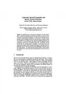
1.6.1 A Setting for Automatic Speech Recognition Figure 1.1 illustrates automatic speech recognition as a process involving several parts. First there is the talker or speaker who is producing the utterance. In this illustration, the utterance is captured by a telephone handset. Next there is the speech recognition system that is connected to the telephone system and is recording the utterance. It performs 2 At http://www.cse.ogi.edu/CSLU/toolkit/documentation/recog/recog.html, as of July 1997.

1.6 Tutorial on Automatic Speech Recognition

8

Typical Automatic Speech Recognition

Talker Utterance

Speech Recog System

Yes No ...

-396 -412 ...

Word Models

Model Decision Scores

Winner

Figure 1.1: A Setting for Automatic Speech Recognition an analysis of the utterance and compares it to the various word models in its active vocabulary. There may be other words and word models that are known by the ASR system which are not included in the active vocabulary because they do not represent expected inputs at this point in time. The word models are indicated by the words \Yes" and \No." The full model includes an actual string of phonemes (a pronunciation) that must be present in the utterance for recognition to occur. For each of these word models a score is computed that re ects the goodness of the match between the utterance and the word model. The method for calculating the score is given below. All word models, even wrong models, will create some score. Finally a decision is made and the model that achieves the highest score is \recognized" as the (putative) winner. The following gures illustrate these steps in greater detail.

1.6.2 Overview of Speech Recognition Figure 1.2 gives an overview of automatic speech recognition.

Upper Left: The utterance is transformed by the telephone (or microphone) into an

electric signal. The waveform of the utterance \two" shows the electrical signal from the

1.6 Tutorial on Automatic Speech Recognition

9

Oregon Graduate Institute of Science and Technology

Overview classify this frame

spectral

context

analysis

window

Viterbi u search

phoneme

t$sil

oU>$sil

trained on: OGI Numbers, Yes/No, Apple, and Stories corpora, and NYNEX PhoneBook corpus. Center for Spoken Language Understanding (CSLU)

Figure 1.3: Arti cial Neural Network. Used by permission.

1.6.3 Arti cial Neural Network Figure 1.3 illustrates the arti cial neural network that is used in the recognition process. For each frame of input, a 5-frame context window is used, with frames oset -6, -3, 0, 3, and 6 from the current frame. The features include MFCC features and delta ( rst-order dierence) MFCC features at the rate of 26 per frame. The rst 12 are mfcc coecients for that frame of speech, and with those is one energy coecient indicating the amount of energy in the signal at that frame. Energy is the RMS (root mean squared) value for the samples in the frame. It is computed by squaring all the sample values, summing the result, and taking the square root. The other 13 numbers are called delta coecients and give the dierence between the mfcc and energy in this frame versus the previous frame. That is, the delta values tell

1.6 Tutorial on Automatic Speech Recognition

13

how much the coecients have changed. The particular input features used will possibly dier from recognizer to recognizer. This totals 130 inputs (plus one hard-wired to a constant value of 1.0). The neural network has 200 hidden nodes and 544 outputs. Table 4.1 on page 47 lists the outputs. Five frames of feature values are used in building a 130-number feature vector for input to the neural network. With each frame occupying 10 msec of the input speech, the total window is 130 msec, about 1/7 of a second. Half of that is involved in look-ahead. That is, the ANN does not make a decision about the current frame until it has seen the next six frames after it. The conversion of input features into phoneme probabilities progresses on a frameby-frame basis. On the top of the diagram the input features are indicated. Each input value is a real-valued number. Conceptually it is loaded into a node in the top row. To compute the value for a node in the center row, each top-row value is multiplied by a weight. The results are added together and then run through a sigmoid function to limit the values to the range -1 through 1. The weights correspond to the lines that connect the nodes. If there are n inputs and m hidden nodes, there will be n  m weights between those two layers in a fully-connected neural net architecture. In this way the values of all the nodes in the hidden layer are computed. Then the bottom row is computed from the hidden-layer values and the next set of intervening weights. The values in the nal layer are outputs. In this gure there are only three layers. Each output corresponds to a single phoneme or to a single phoneme state (half or a third of a phoneme). Taking the rst output, /pau/, for example, the value there might be .34. This would indicate that the inputs provided have about a 34% chance of representing the /pau/ (pause or silence) phoneme. A chart showing the phoneme set appears on page 62.

1.6.4 Context-Dependent Modeling Figure 1.4 examines context-dependent modeling. Each context-dependent phoneme is divided into one, two, or three parts. For example, the word \yes" is given as three phonemes: /j E s/. (/j/ is the Worldbet symbol for the \y" sound. See Table 4.3 on page 62

1.6 Tutorial on Automatic Speech Recognition

14

Oregon Graduate Institute of Science and Technology

Context-Dependent Modeling (vocabulary independent) divide each phoneme into 1, 2, or 3 parts. example: "yes" /y E s/: $sil$fric /E/ model

current phoneme

/E/ left

/E/

/E/

middle right

8 broad contexts

$mid$sil

next phoneme front mid back sil nasal retro fric other

8 broad contexts

17 categories per 3-part phoneme Center for Spoken Language Understanding (CSLU)

Figure 1.4: Context-Dependent Modeling. Used by permission. for a presentation of those symbols.) The /j/ phoneme is divided into two parts: j-aftersilence and j-before-mid-vowel. The /E/ phoneme is divided into three parts: E-afterfront-vowel, central-E, and E-before-fricative. The /s/ phoneme is divided into two parts: s-after-mid-vowel and s-before-silence. Including mid-vowel, front-vowel, and fricative, there are eight broad contexts with which to identify the previous phoneme and the next phoneme. This list of contexts can vary by phoneme for maximum usefulness.

1.6.5 Viterbi Search Example Figure 1.5 illustrates two search paths created by Viterbi search. In this example, the search paths for \yes" and \no" are shown, on a eld of thirteen ANN outputs and twenty speech frames. In each cell, the darkness indicates the probability contribution from that cell. The Viterbi algorithm searches through the cells to nd the path with the highest

1.6 Tutorial on Automatic Speech Recognition

15

Oregon Graduate Institute of Science and Technology

Viterbi Search Example search paths for "yes" and "no"

neural network output matrix

$sil$mid $mid$sil n>$back oU>$sil $sili|^|@|E|ei|I|i:)3 are designated to be proto-syllables. Diphthongs are not divided because they already represent a single phoneme. Adjacent vowels in dierent phonemes are established as separate syllable nuclei. 2. Zero or one liquids (j|9r|w|l) that occur immediately before proto-syllables are merged in, making those proto-syllables larger. 3. Zero or one (b|d|g|ph|th|kh|tS|dZ|f|S|T|D|v|z|h|d_(|j|m|n) that occur immediately before proto-syllables are merged in next. 4. Zero or one (s) that occur immediately before proto-syllables are merged in next. 3 For a de nition of the phonemes, please see Table 4.3.

5.4 Segmental Averaging

104

5. Zero or one (S) that occur immediately before (m|n) in proto-syllables are merged in next. These occur in words like Schneider. 6. All unused (b|d|g|ph|th|kh|tS|dZ|s|f|S|T|D|v|z|h|d_(|j|9r|w|l|m|n) that occur immediately after proto-syllables are merged in. At this point all phonemes have been merged into proto-syllables, which can now be called syllables. 7. Occurrences of (9r l) are split into separate syllables. These occur in words like girl, charles(ton), and carl. This is a dialect-speci c issue and could be done with or without a syllable boundary in these contexts. This seemed a good place to start. This overall algorithm as stated seems to work well with word models from Orator TTS and word models from CMU dictionary, which are used with the Names and PhoneBook corpora respectively. It was spot-tested on a number of words and seemed to have a high accuracy rate. This suggests that it would give a performance indicative of its full value had greater care been taken. The algorithm was not extensively tested. Table 5.6 shows that fspsw results are about 1% worse than fspw ( = .1252) which is not a signi cant dierence. This performance did not seem to justify additional careful study of syllable clustering algorithms at this time.

Conclusions: Table 5.7 shows that for the ? log(pr ) algorithm any type of sub-word

averaging is clearly a big win in comparison to fw averaging. This is believed to be due to the presence of insertion-type errors which have been observed during review of impostor segmentations. The review is not dramatically conclusive and is not presented in this thesis but suggests that impostor segmentations often contain short phonemes with very bad scores amid much longer phonemes that are largely correct. By averaging across phonemes each phoneme or segment is treated equally so the longer ones no longer overpower the short ones. By extension this conjecture would imply that averaging across sub-word units will help if the units are of substantially varying length. (With units of roughly equal length averaging will have no eect.) This seems to be borne out by the good performance of fspw which continues to be unsurpassed among the results yet to be reported in this thesis. It merges a widely varying number of frames into each segment, and merges from one to

5.5 On-Line Garbage Improved

105

three segments into a phoneme. However it is disappointing that the fspsw method with syllables of greatly varying length does not make a further improvement. This could be due to an incorrect approach to identifying syllable boundaries, or an inappropriate choice of test corpora. In any event, the dierence is not signi cant nor is it large. Based on these conclusions performance using fspw is presented hereafter for

comparison among algorithms.

The frame/segment/phoneme/word averaging performance of ? log(pr ) (.1233.0013) is better than its frame-to-word averaging performance (.1639.0012). The use of segmental accumulation strategies accounts for this improvement. The performance even surpasses the whole-utterance on-line garbage scoring performance of g(4,16) (.1554.0013), the top whole-word on-line garbage model. It seems possible that segmental accumulation coupled with -based normalization might create a further improvement. This is examined in section 5.5.

5.5 On-Line Garbage Improved The concept here is to normalize each frame score pr by some identi able score or group of scores in the frame. This is like comparing to the whole-word garbage score at an estimated rank (section 5.2), but diers in several respects. First, the normalization occurs on a frame by frame basis rather than a whole word (or whole utterance) at a time. The use of frame-based normalization makes it possible to average within segments, which has been shown in section 5.4 to improve performance. Second, the equivalent rank is not computed, but rather by how much the frame score diers from some speci ed score. Third, the modeled portions of the utterance are not included in the calculation, thus removing any noise they may have been contributing. Normalization in this way bears a resemblance to acoustic normalization required by Bayes rule: p(W jA) = p(AjW )p(W )=p(A). In this formulation p(AjW ) is normally provided by an HMM and is often called a likelihood. p(W ) is the (a priori ) probability of occurrence for word W and is often provided by a language model. The probability

5.5 On-Line Garbage Improved

106

p(A) of the observed acoustics A is often neglected in choosing the best word hypothesis because it is the same for all word hypotheses for that utterance (i.e., the acoustics are the same no matter what words are hypothesized). In theory p(A) can be computed by summing all the p(AjW )p(W ) since the total probability is 1.0 by de nition. In practice there are too many words W to be considered. If phonemes or sub-phonetic units are used instead of words it becomes possible to sum them all. p(A) might also be estimated (modulo an unknown constant multiplier) by the methods of this section. Because of restrictions in the training of the ANNs used as recognizers in this thesis (see section 4.1.2), it is possible that the a posteriori probabilities generated by the ANN are not fully a posteriori at all, but could still bene t from such a normalization as this. If on the other hand they are true a posteriori probabilities, the value p(A) estimated by the methods of this section should be approximately constant and will therefore have little or no eect on performance.

5.5.1 Initial Experiments The rst experiments were performed normalizing against scores at median 10, 20, and 50 (ranks 6, 11, and 26 respectively). Low4 median values were chosen because they were expected to be more stable, and thus better normalization factors. Part A of Table 5.8 shows that the EER varies across these experiments and that log(pr =g (R6)) performed the best of the three at .1138.0013.

5.5.2 High Ranks Because the highest rank seemed to perform better, additional experiments were performed at ranks 1, 2, 3, 4, and 5, to study how performance varies with rank. Part B of Table 5.8 shows that log(pr =g (R2)) performs the best (nominally) at .1118.0013, but that there is not a statistically signi cant dierence among these normalization alternatives. 4 Rank 1 is the highest rank.

5.5 On-Line Garbage Improved

107

Table 5.8: Distance Chart for Algorithms in the log(pr =g (low)) and log(pr =g (high)) Families. Notice that higher ranks seem to produce better performance, but the top ranks all performed about the same. Details: impostors at perplexity 20, Oct 1996 MFCCbased recognizer, equal mix of OGI Names corpus and NYNEX PhoneBook corpus, frame/segment/phoneme/word averaging, word models depending on corpus, 32000 trials, nal test set, equal error rates. For more explanation see page 72. Part A: log(pr =g (low)) Family .1138.0013, log(pr =g (R6)) 1 .1178.0013, log(pr=g(R11)) 10 6 .1292.0014, log(pr =g(R26)) Part B: log(pr =g (high)) Family .1118.0013, log(pr =g (R2)) 0 .1118.0014, log(pr=g(R3)) 0 0 .1128.0014, log(pr =g(R4)) 0 0 0 .1133.0013, log(pr =g(R5)) 0 0 0 0 .1138.0013, log(pr =g(R6)) 0 0 0 0 0 .1143.0014, log(pr =g(R1))

5.5.3 Averages of High Ranks Because averaging several numbers tends to reduce variability (e.g., improves the reliability), averaging the top few ranks seemed to promise further performance gains. Experiments were performed averaging ranks (1..2), (1..3), (1..4), and (2..3). Averaging was performed in the logarithm domain (the average of the log-probabilities of the speci ed ranks was subtracted from log(pr )). Part A of Table 5.9 shows log(pr =g (R1::4)) with performance of .1115.0013 emerging as the new nominal leader. The marginal improvement over log(pr =g (R2)) at .1118.0013 is not signi cant.

5.5.4 Wider Averages The log(pr =g (R1::4)) average gave the most promising results, but the other averages were almost identical. Additional experiments were then performed averaging across ranks (1..10), (1..20), (1..30), (1..40), and (1..50) to assess the usefulness of larger groupings and the eects of lower ranks for computing the normalization factor. Part B of Table 5.9 shows that performance suers signi cantly as the lower ranks become involved in the

5.5 On-Line Garbage Improved

108

Table 5.9: Distance Chart for Algorithms in the log(pr =g (few)) Family. Notice that ranges of the top ranks performed about the same, but that as lower ranks become involved performance declines. Details: impostors at perplexity 20, Oct 1996 MFCCbased recognizer, equal mix of OGI Names corpus and NYNEX PhoneBook corpus, frame/segment/phoneme/word averaging, word models depending on corpus, 32000 trials, nal test set, equal error rates. For more explanation see page 72. Part A: log(pr =g (few)) Family .1115.0013, log(pr =g (R1::4)) 0 .1117.0015, log(pr =g(R2::3)) 0 0 .1119.0015, log(pr =g(R1::3)) 0 0 0 .1129.0014, log(pr=g(R1::2)) Part B: log(pr =g (many )) Family .1137.0015, log(pr =g (R1::10)) 0 .1160.0014, log(pr =g(R1::20)) 2 0 .1192.0014, log(pr =g(R1::30)) 4 2 0 .1221.0012, log(pr=g(R1::40)) 6 4 2 0 .1250.0013, log(pr=g(R1::50)) averaging. This suggests that the lower ranks are not as good a standard for comparison as are the upper ones. These experiments substantiate a steady trend with (1..10) being best and (1..50) being worst.

5.5.5 Experimental Details Motivation: On a frame-by-frame basis the frame probability can be normalized by

another score to accentuate how much better or worse it is. The intuition is that ANN performance can be aected by the acoustic quality of the utterance. A noisy utterance can be expected to have worse scores overall than a clean utterance. An unusual speaker can be expected to have worse scores overall than a speaker who is similar to those used in training. It is hypothesized that all important scores will rise or fall together with the acoustic quality of the utterance, and that this fact can be exploited for reliable normalization. If the normalizing score is a consistent baseline (such as the on-line garbage score) then the revised score should indicate improvement over random chance, given the waveform present in that frame.

5.5 On-Line Garbage Improved

109

De nition: The individual frame score f is computed by dividing the raw a posteriori

probability pr by a normalizing factor (the nth ranking score or an average of such scores in that same frame). The identities of the normalizing scores are varied across experiments. Speci cally the f = log(pr ) minus the mean of the logarithms of the scores at the normalizing ranks.

Hypothesis 1: Normalizing by a garbage score computed in this manner allows discrimination between correct and incorrect recognitions.

Hypothesis 2: Segment-based averaging is more accurate than whole-word averaging. Hypothesis 3: Performance varies signi cantly as a function of the normalizing scores used.

5.5.6 Discussion and Conclusions Performance varies signi cantly as a function of the normalizing scores used. Across singlerank algorithms, the top ranks consistently outperform the lower ranks, except that rank 1 is apparently worse than ranks 2 through 6. The cause for this reversal is not understood. Among rank-range algorithms, those concentrated in the highest ranks consistently perform best. The speci c choice of ranks involved does not seem to be very sensitive. As anticipated the combination of segmental accumulation and -based normalization has created a further improvement. The performance of log(pr =g (R1::4)) (.1115.0013) is 10% better than the performance of ? log(pr ) (.1233.0013).

Chapter 6 Vocabulary-Independent Rank-Based Algorithms This chapter presents new research in the area of rank-based probability estimation. These experiments represent new research in the eld of speech recognition. It continues the format of the previous chapter where baseline performance results were developed. It uses the general methodology described in chapter 4. At the end of this chapter, a section of nal results presents the top results from all the experiments that have been reported. Rank by itself is an indicator of recognition quality. On a frame-by-frame basis, the ANN output used will have some rank R with respect to all ANN outputs pr in that frame. (Note that R will be used to signal \rank." This should not be confused with the use of r for \raw" which occurs in the context pr .) It is hypothesized that a rank of 1 means the same thing whether the absolute score pr is 0.6 or 0.2. In particular, rank should be robust to acoustic variations in the incoming speech signal. The intuition is that background noise, microphone quality, and speaker enunciation aect the absolute scores much more than they aect the relative scores or rankings of the phonemes. If this is true then rank will be a better indicator of recognition accuracy than the absolute score is. This section will examine a family of algorithms based solely on the frame-by-frame rank of the phonemes in the word model. Rank is computed in the most simple and obvious way. The ANN output value pr is compared to all other values in that frame, and the number of values that are equal or greater becomes the rank. Ranks range from 1 (high) to 544 (low) for the Oct96 recognizer. 110

6.1 Estimating Probability Three Ways

111

Given the rank, it is desirable to convert it back into some form of probability for accumulation, since I have already shown that averaging the logarithms of probabilities (see section 5.3) across segments and then phonemes (see section 5.4) gives a good performance. The conversion to probability will be done using the a priori probabilities of observing those ranks in correct words or in impostors. This allows me to directly model the accuracy of phoneme ranks in the correct-word and out-of-vocabulary settings. The probabilities are trained using a corpus. The value pr is not used except to determine the rank. Only the rank and the identity of the phoneme are used in computing the frame scores.

6.1 Estimating Probability Three Ways Three ways are used to formulate probability for these experiments. The most obvious way is the likelihood ratio or odds (p(true)/p(false)). Other ways are simple probability (p(true)) and cumulative probability.

6.1.1 p(true), p(false) The probability of truth and falsehood are de ned dierently than they were for pn =(1?pn ) in section 4.8.3. There the ANN output values were normalized in each frame, and the phoneme used by the word model (pn ) represented truth while the sum of all the rest (1 ? pn ) represented falsehood.

p(true): Here the probability of truth is de ned as the frequency of occurrence of some

rank R across a training set of correctly recognized words. If the phoneme x occurs in 1000 frames in that training corpus, and if it has a rank of 1 in 270 of those frames, then p(rank=1|truth) is .27. To compile these statistics, all utterances in the training set were used. Each word was recognized using its correct word model. For each frame two things were noted: (a) what is the correct phoneme (ANN output), and (b) what rank does it have. After performing this forced alignment process for all words in the training set, the results were separated by phoneme (ANN output). Since there are 544 ANN outputs, this resulted in 544 separate lists. Each list gives the ranks that were observed when that

6.1 Estimating Probability Three Ways

112

Phoneme 21 (n=650) 1

Cumulative Probability

data cubic 0.1

0.01

0.001 1

10 Rank

100

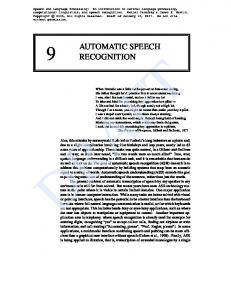
Figure 6.1: Cumulative Probabilities M (R) for Phoneme 21. Notice the close t for higher ranks. Ranks not shown had zero cumulative frequency. Details: Oct 1996 MFCCbased recognizer, all training set words from OGI Names corpus and NYNEX PhoneBook corpus, word models depending on corpus. ANN output was actually true. The largest portion of the ranks were 1. Figure 6.1 shows the distribution of these ranks for ANN output 21, where there were 650 frames in the training set that were found to match that ANN output. Figure 6.2 shows the distribution of these ranks for ANN outputs 3, 23, and 36. Phoneme 36 commonly gives inaccurate rankings even when the phoneme is correct. Phoneme 3 changes from accurate rankings at the high end to inaccurate rankings at the low end. Phoneme 23 gives consistently accurate rankings through the full range shown. This suggests that phoneme 23 is well trained in the ANN, but phoneme 36 is poorly trained.

p(false): The probability of falsehood is estimated across a training set as well. In this

case, each utterance was falsely recognized as the best-matching word from a list made of

6.1 Estimating Probability Three Ways

113

Variation Among Phonemes in Probability per Rank

Cumulative Probability

1 phoneme 36 phoneme 3 phoneme 23 0.1

0.01

0.001 1

10

100 Rank

Figure 6.2: Variations Among Phonemes in Cumulative Probability M (R) per Rank. Notice that phoneme 36 commonly gives inaccurate rankings even when the phoneme is correct. Phoneme 3 changes from accurate rankings at the high end to inaccurate rankings at the low end. Phoneme 23 gives consistently accurate rankings through the full range shown. Details: Oct 1996 MFCC-based recognizer, all training set words from OGI Names corpus and NYNEX PhoneBook corpus, word models depending on corpus. random incorrect words. Because of the time required to collect this list (many times longer than for the true words) some preliminary experiments were done to determine the best number of wrong words to place in the set from which the impostor would be drawn. Experiments were done with perplexity 2, 20, and 1000. It was seen that between 2 and 20, there was improvement at 20, but between 20 and 1000 the performance was not much dierent. This could be checked further but due to the time cost of the experiments I concluded based on early results that perplexity 20 would give an adequate indication of the merits of this approach. For each impostor word, the frames were examined individually. The designated

6.1 Estimating Probability Three Ways

114

phoneme (ANN output) was either correct or not. This was determined by comparison to the alignment of the correct word model for that utterance. If the impostor and the correct word model speci ed the same phoneme, then the phoneme was correct, even though it appeared in the impostor word. This occurred in the word pair \foil" versus \coil," where the majority of the frames in the impostor were actually correct. After the correct frames were eliminated, the remaining (incorrect) frames were again examined. For the phoneme used in the impostor, the rank was computed and added to a list for that phoneme. This resulted in 544 lists of ranks, where each rank was an actual observed rank for the phoneme in question, in an impostor word, and was not the true correct phoneme for that frame.

Choice of Impostors An important question remains unanswered. That is the question

of how best to select impostors. Ideally the impostors would follow the same distribution what would occur naturally when an out-of-vocabulary utterance is given to a randomly chosen task-speci c recognizer. Unfortunately it is not known how to create task-speci c recognizers at random, and how to create the kinds of OOV utterances that such recognizers might encounter. Even the selection of a random set of tasks for which task-speci c recognizers could be constructed seems intractable. Therefore as a rst approximation the utterances were chosen at random and applied to a task-independent vocabulary also chosen at random. However, this cannot be more than a rst approximation due to the problems with correctly characterizing impostor recognitions.

Summary: The probability of falsehood is estimated across a training set of impostors

at perplexity 20. Other perplexities were examined but the results do not seem to be particularly sensitive to this choice. The choice of impostors remains an important and unsettled issue. If the phoneme x occurs in 1000 frames in that training corpus, and if it has a rank of 1 in 80 of those frames, then p(rank=1|falsehood) is .08. In any frame where the impostor phoneme is the same as the true phoneme, the

6.1 Estimating Probability Three Ways

115

phoneme 21 (t=602, f=398) 10

likelihood ratio

data cubic 1

0.1

0.01 1

10 rank

100

Figure 6.3: Likelihood Ratios `P (R) for Phoneme 21. Notice the poor t for lower ranks. Ranks not shown had zero frequency. Details: impostors at perplexity 20, Oct 1996 MFCC-based recognizer, all training set words from NYNEX PhoneBook corpus, word models depending on corpus. impostor is ignored. This helps prevent foil/coil problems, where the true word is \foil," the impostor is \coil," and the \oil" frames should not be counted as both true and impostor. Instead they are counted only as true.

6.1.2 Cubic Polynomial Smoothing Few trues occur at low ranks. For that matter few falses occur at low ranks either. Smoothing is critical to estimate reasonable probabilities in the low-rank tail of these distributions. For each ANN output a separate probability curve was tted, using a cubic polynomial taking the logarithm of rank as the independent variable and returning the logarithm of the probability. Examples are shown in gures 6.3 and 6.1.

6.1 Estimating Probability Three Ways

116

6.1.3 Likelihood Ratio Likelihood Ratio is denoted by `P (R). (The P indicates PhoneBook training.) It identi es a set of 544 cubic polynomials trained to estimate the logarithm of the likelihood ratio of the PhoneBook corpus training set given the logarithm of the rank. The likelihood ratio in the above case would be ::27 08 , which combines with the prior likelihood pp((ft)) to yield the likelihood given the observed rank. The typical assumption is that truth and falsehood are equally likely so pp((ft)) = 1 and it cancels out of the equation 27 as the likelihood given the observed rank. leaving just ::08 Figure 6.3 illustrates the t between data observed and the cubic polynomial. For most of the 544 phonemes the t was better and n was larger but the tail of righthand the curve still came up. Much more data may be required to get a reliable distribution.

6.1.4 Simple Probability Simple Probability is denoted by S P (R) (for PhoneBook training) or S M (R) (for Mixed training). The simple true probability in the above case would be .27. The probability of falsehood does not enter into the calculation. This is expected to be less accurate than the likelihood ratio, but given the fundamental problems with generation of impostors, simple probability is an interesting alternative worth examining.

6.1.5 Cumulative Probability This is denoted by P (R) (for PhoneBook training) or M (R) (for Mixed training). Each identi es a set of 544 cubic polynomials trained to estimate the logarithm of the cumulative probability of the training corpus set given the logarithm of the rank. The cumulative true probability is perhaps the most interesting alternative. It takes into account the belief that higher rank implies a better match. This seems obvious, but it is not used in either the likelihood ratio formulation nor in the simple probability formulation. In the cumulative formulation, probability is the sum of the simple probability at that rank and at all lower (worse) ranks. Thus by de nition the cumulative probability of truth at rank 1 is always 1.0. In the above case, the cumulative probability at rank 2

6.2 Probability Training Corpus Selection

117

Table 6.1: Distance Chart for Algorithms in the f P (R) Family. Notice that cumulative is nominally better but only by an insigni cant margin. Details: impostors at perplexity 20, Oct 1996 MFCC-based recognizer, equal mix of OGI Names corpus and NYNEX PhoneBook corpus, frame/segment/phoneme/word averaging, word models depending on corpus, 32000 trials, nal test set, equal error rates. For more explanation see page 72.



P (R)) 0 .1225.0014, Mean(`P (R)) 1 0 .1230.0014, Mean(S P (R)) .1195 .0014, Mean(

would be 1.0-.27=.73. Figure 6.1 illustrates the t between data observed and the cubic polynomial. For most of the 544 phonemes the t was better and n was larger.

6.1.6 Estimating Simple Probability To get the simple (non-cumulative) proportion of scores at a certain rank a \delta cumulative" approach is convenient. Because of sparse data in the lower ranks, and the convenience of having the cumulative curve already tted, the probability at any rank R is estimated as the cumulative probability at that rank minus the cumulative probability at rank (R + 1). This is exactly the original probability at that rank, but smoothed to adjust for sparsity of data.

6.2 Probability Training Corpus Selection It is not immediately clear which approach should yield the best performance. The frame scores play together in complicated ways. A variety of experiments will be performed to try to create some intuition about the relative behaviors. The rst experiment tests to see which of these probability formulations is best, or whether they are not distinguishable. The probabilities are trained using PhoneBook. Table 6.1 shows that cumulative is better by an insigni cant margin. Mean(`P (R)) was eliminated from consideration at this point because the approach is very computationally expensive, requiring 500 times more impostors to train compared to the cumulative approach, and not yielding any improvement in performance. Therefore, results were generated for `P (R) but not `M (R).

6.2 Probability Training Corpus Selection

118

Table 6.2: Distance Chart for Algorithms in the f M (R) Family. Notice that Mixed training is signi cantly better than PhoneBook training. Details: impostors at perplexity 20, Oct 1996 MFCC-based recognizer, equal mix of OGI Names corpus and NYNEX PhoneBook corpus, frame/segment/phoneme/word averaging, word models depending on corpus, 32000 trials, nal test set, equal error rates. For more explanation see page 72.



M (R)) .1171.0013, Mean(S M (R)) 0 .1195.0014, Mean(P (R)) 2 0 .1225.0014, Mean(`P (R)) 2 1 0 .1230.0014, Mean(S P (R))

.1144 .0014, Mean(

0 2 4 4

Table 6.3: Distance Chart for Algorithms in the f (R) Family. Notice that Mixed training still appears to be better than the PhoneBook training, although the results are not as signi cant. Details: impostors at perplexity 20, Oct 1996 MFCC-based recognizer, NYNEX PhoneBook corpus, frame/segment/phoneme/word averaging, word models from CMU dictionary, 16000 trials, nal test set, equal error rates. For more explanation see page 72.



M (R)) .0595.0012, Mean(P (R)) 0 .0617.0014, Mean(S M (R)) 2 1 .0658.0015, Mean(S P (R)) 3 1 0 .0659.0013, Mean(`P (R))

.0587 .0015, Mean(

0 0 3 3

The second experiment tests whether using NYNEX PhoneBook corpus is better, or whether equal mix of OGI Names corpus and NYNEX PhoneBook corpus is better. Table 6.2 shows that Mixed provides signi cantly better training for both (R) (=.0089) and S (R) (=.0024). This indicates that \more data is better." However, it also raises a question on whether this result is due to testing with the Mixed corpus. The third experiment tests whether these results hold up when tested against the PhoneBook corpus. That is, when the probabilities are trained on corpus x do they simply perform better on corpus x? Table 6.3 shows that Mixed training still appears to be better than the PhoneBook training, although the results are not as signi cant. It is still reasonable to believe that Mixed training is better. The Mean(`P (R)) turns in a

6.3 Weighted Alternatives to Mean Accumulation

119

particularly poor showing on this set, which does not bode well for its long-term abilities.

6.3 Weighted Alternatives to Mean Accumulation Up to this point averaging has been done in the ordinary way, with perhaps a change to the logarithmic domain to get a geometric mean. The geometric averaging has been shown to contribute to performance for the averaging of probabilities. Review of the actual ranks obtained on a segment by segment basis showed that at the beginning and end of correct segments the ranks tended to be poor, but in the middle of each segment the ranks were high. This indicates that the ANN transitions are still a problem as the processing moves from segment to segment. This section of experiments looks at several alternative ways to perform averaging. It is motivated by examination of the actual probabilities that make up the scores for trues and impostors. Based on visual observation it was hypothesized that impostors have a higher proportion of bad frame scores. To test this hypothesis three alternate forms of averaging were created. For each of these forms of averaging the raw probabilities are rst sorted within the segment, and are then weighted according to their position in the sorted sequence. Better scores appear rst and are weighted more lightly. Worse scores appear last and are weighted more heavily. Following are the weighting schemes used.

6.3.1 Mean Averaging In mean averaging the weights are constant. For n frames, each is weighted by 1. The sum is divided by the sum of the weights (n). This is common, ordinary averaging. It is the baseline for comparison with the experimental forms of averaging. The mean average score is roughly equal to one of the middle score in the set.

6.3.2 Triangular Averaging In triangular averaging the weights increase by one for each additional item, starting from a base of zero. For n frames, the best is weighted by 1, the next by 2, then 3, and so on to the last which is weighted by n. The sum is divided by the sum of the weights ( n(n2?1) ).

6.3 Weighted Alternatives to Mean Accumulation

120

By doing a triangular form of averaging, the worse scores have much more eect on the nal segment score than do the better scores. The idea is that better scores are simply expected and should not be rewarded, but the worse scores are a violation of expectations and should be penalized. The triangular average score is roughly equal to one of the worse scores in the set.

6.3.3 Trapezoidal Averaging In trapezoidal averaging the weights increase by one for each additional item, starting from a base of n. For n frames, the best is weighted by n + 1, the next by n + 2, and so on to the last which is weighted by 2n. The sum is divided by the sum of the weights. By doing trapezoidal averaging the good scores make a larger contribution to the average than under triangular averaging. Trapezoidal is a compromise between triangular and mean averaging. The trapezoidal average score is roughly half way between the mean average score and the triangular score.

6.3.4 Parabolic Averaging In parabolic averaging the dierence between weights increases by one for each additional item. For n frames, the best is weighted by 1, the next by 2, then 4, then 7, then 11, and so on. The nth is weighted by 21 x2 ? 12 x +1. The sum is divided by the sum of the weights. By doing parabolic averaging the bad scores make a larger contribution than under triangular averaging. This is yet more extreme than triangular averaging, and approximates selecting the next-to-worst score as the representative for the entire segment.

6.3.5 Usage Mean, triangular, trapezoidal, and parabolic forms of averaging are evaluated in the next two sections. In section 6.4 the rank numbers (1, 2, 3, : : : ) are averaged before converting to the probability domain. In section 6.5 the ranks are converted to probabilities rst and then the averages are computed.

6.4 Averaging Ranks

121

Table 6.4: Distance Chart for Algorithms in the f (av (R)) Family. Notice that more exotic averaging (trapeziodal, triangular, parabolic) has not improved performance. Details: impostors at perplexity 20, Oct 1996 MFCC-based recognizer, equal mix of OGI Names corpus and NYNEX PhoneBook corpus, frame/segment/phoneme/word averaging, word models depending on corpus, 32000 trials, nal test set, equal error rates. For more explanation see page 72.



M (Mean(R)) 0 .1165.0014, M (Trap(R)) 0 0 .1175.0014, M (Tri(R)) 0 0 0 .1182.0014, M (Para(R)) .1164 .0013,

6.4 Averaging Ranks In this experiment the ranks themselves were averaged before computing the probability. For those cubic polynomials that are largely straight across the range of ranks involved, this will be the same as averaging the logarithms of the probabilities. In other cases it will make a dierence. This experiment is motivated by the visual observations made while examining the phoneme ranks for trues and impostors. Those observations seemed to indicate that incorrect alignments had more bad scores than correct alignments did. I hypothesized that averaging the ranks would perform dierently from averaging the probabilities (discussed in section 6.5). Table 6.4 shows that exotic averaging (trapezoidal, triangular, parabolic) has not improved performance. In fact, as the weighting becomes more extreme the performance appears to drop more. Thus mean with the least weighting dierence performs best, and parabolic with the most weighting dierence performs worst. Unfortunately there is not enough accuracy in the numbers to draw solid conclusions. Therefore this observation is preliminary.

6.5 Averaging Probabilities In this experiment the logarithms of probabilities were averaged. For those cubic polynomials that are largely straight across the range of ranks involved, this will be the same

6.6 Conclusions

122

Table 6.5: Distance Chart for Algorithms in the av (f (R)) Family. Table 6.4 results are included for comparison. Notice that computing probabilities before averaging seems to improve performance. Details: impostors at perplexity 20, Oct 1996 MFCCbased recognizer, equal mix of OGI Names corpus and NYNEX PhoneBook corpus, frame/segment/phoneme/word averaging, word models depending on corpus, 32000 trials, nal test set, equal error rates. For more explanation see page 72.



M (R)) .1146.0014, Trap(M (R)) 0 .1149.0014, Tri(M (R)) 0 0 .1164.0013, M (Mean(R)) 0 0 0 .1165.0014, M (Trap(R)) 0 0 0 0 .1175.0014, M (Tri(R)) 1 0 0 0 0 .1182.0014, M (Para(R))

.1144 .0014, Mean(

0 0 0 0 0 1

as averaging the ranks as reported in section 6.4. In other cases it will make a dierence. I hypothesized that averaging the ranks would perform dierently from averaging the probabilities (discussed in section 6.5). Table 6.5 shows that computing log-probabilities before averaging seems to improve performance, and the exotic averaging (trapezoidal and triangular) still seem to fall behind the simple mean average. However, the dierences between all these results are too weak to be conclusive.

6.6 Conclusions It can be seen that Mean(M (R)) (.1144.0014) has good performance. In fact the performance is not signi cantly dierent from log(pr =g (R1::4)) (.1115.0013). It is interesting to see that rank alone is able to achieve this quality of result. Exotic forms of averaging do not seem to improve performance. Averaging ranks rather than probabilities does not improve performance. Further, averaging that weights each item equally appears to perform better than averaging that emphasizes items with lower scores. Mean averaging appears to be best.

6.7 Vocabulary-Independent Final Results

123

Cumulative probabilities show promise in comparison to simple probabilities and likelihood ratios, but the results are not conclusive. A larger number of trials is required to see whether these apparent dierences are real.

6.7 Vocabulary-Independent Final Results Table 6.6 presents the top results from all the experiments that have been reported in the previous several chapters on vocabulary-independent experiments. They are shown using three separate evaluation sets: Names, PhoneBook, and Mixed. To be concise only the top performers are presented, using the fspw and fw accumulation strategies and impostors at perplexity 20. Preliminary results using the development test set show that the algorithms best at this perplexity are also best at other perplexities. Final results were limited to perplexity 20 only.

6.7 Vocabulary-Independent Final Results

124

Table 6.6: Distance Chart for the Top Algorithms. Details: impostors at perplexity 20, Oct 1996 MFCC-based recognizer, nal test set, equal error rates. For more explanation see page 72. NYNEX PhoneBook corpus word models from CMU dictionary, 16000 trials .0587.0015, Mean(M (R)) fspw 0 .0591.0015, log(pr=g(R1::4)) fspw 3 3 .0664.0015, ? log(pr) fspw 13 13 7 .0803.0016, log(pr=g(R1::4)) fw 18 18 14 3 .0893.0016, Mean(M (R)) fw

19 21 37 36

19 21 36 36

14 17 35 35

4 8 32 34

0 .0910.0017, g(4,16) fw 2 1 .0967.0018, ? log(pr ) fw 29 28 26 .1524.0017, pr fspw 32 32 31 21 .2216.0021, pr fw

equal mix of OGI Names corpus and NYNEX PhoneBook corpus word models depending on corpus, 32000 trials .1115.0013, log(pr =g (R1::4)) fspw 0 .1144.0014, Mean(M (R)) fspw 7 5 .1233.0013, ? log(pr) fspw 21 19 13 .1414.0013, log(pr=g(R1::4)) fw 24 22 18 4 .1503.0015, Mean(M (R)) fw

27 30 40 49

26 29 39 48

22 26 38 48

10 17 34 46

2 .1554.0013, g(4,16) fw 9 5 .1639.0012, ? log(pr ) fw 31 30 28 .2097.0014, pr fspw 43 44 43 33 .2755.0014, pr fw

OGI Names corpus word models from Orator TTS, 16000 trials .1648.0023, log(pr =g (R1::4)) fspw 0 .1661.0019, Mean(M (R)) fspw 4 4 .1791.0022, ? log(pr) fspw 17 18 11 .2051.0021, log(pr=g(R1::4)) fw 18 19 13 1 .2117.0025, Mean(M (R)) fw

21 24 30 34

22 26 31 34

17 21 28 32

4 10 22 29

1 .2176.0022, g(4,16) fw 6 3 .2294.0022, ? log(pr ) fw 19 18 13 .2614.0025, pr fspw 27 27 25 17 .3200.0023, pr fw

Chapter 7 Con dence Rejection by raw thresholds may be a completely adequate solution for many situations in automatic speech recognition. But \tuning" to nd the right setting can be dicult. It can depend on the makeup and size of the impostor vocabulary, as well as the cost analysis of making dierent types of errors. Vocabulary independence and integration with higher processes such as a dialogue manager further increases the diculty of using raw thresholds. Con dence provides a uniform approach to these issues. This chapter completes the discussion of rejection by developing an actual con dence score that can for example guide higher-level decisions about dialogue processing.

7.1 Continuous Versus Discrete The nal use of any con dence and rejection calculation is probably a discrete decision to do one thing or do something else. It seems useful to view \con dence" as a continuum of scores with some designated threshold such that computed scores on one side are \good enough" (accepted) for some purpose, and on the other side they are \not good enough" (rejected). What information should be returned from a con dence and rejection calculation? Is a con dence measure necessary?

7.1.1 Accept, Verify, or Try Again One approach to con dence and rejection is to set two thresholds. The best-scoring recognitions are automatically accepted. The worst-scoring recognitions are automatically rejected. In a voice response system, rejection would generally cause the prompt to be 125

7.2 True Con dence

126

repeated. The middle-scoring recognitions might be veri ed by a dialogue such as, \Did you say (the thing recognized)?" At any given threshold there is some proportion of correct recognitions that will be rejected, and some proportion of incorrect recognitions that will be accepted. Depending upon the application, there may be dierent penalties for dierent system errors. For example, if the question is, \Did you say `Delete all les'?", one might wish to err on the side of caution and only accept a \yes" that is clearly a \yes." But if the response seems to be \no," one might wish to generously accept it, possibly requiring a frustrated user to repeat the command. To err on the side of caution, it is clear that the making of an accept-verify-reject decision requires task-speci c information. The scope of this thesis is to develop general techniques that are applicable in a broad variety of settings. Therefore the veri cation (or \con dence") component is designed to report the probability of some speci ed answer. Other components can be constructed as needed to respond to that assessment.

7.2 True Con dence The goal is to create a con dence measure that can be used by other processes in a straightforward way. One obvious de nition for con dence is the posterior probability that a given recognition event is correct. Because probabilities are equivalent to likelihood ratios,1 and because prior probabilities and task-speci c cost information may not be known, con dence will instead be presented as a likelihood ratio `. Speci cally `(score) = p(scorejtrue) p(scorejimpostor) . These probabilities can be estimated from a training set. Notice that prior probabilities for words and larger constructs are not available for the analysis of this thesis. The availability of prior probabilities is limited to the occurrence of phonemes and strings of phonemes in English. Task-based or vocabulary-based prior probabilities together with updating information from the acoustic reliability scores (con dence measures) created here can be used to generate posterior probabilities. Such use is illustrated in the collect-call example of this thesis, but a detailed consideration of 1 For probability p, the likelihood ratio ` is ` = p . Similarly p = ` . 1?p 1+`

7.2 True Con dence

127

posterior probabilities is beyond the scope of this thesis.

7.2.1 Estimating p(Impostor) Impostors are generated from random lists of incorrect words. As more words are used in each list, the chance of getting a better impostor is improved. With a list of one word, that word becomes the impostor. With the addition of a second word, there is a 50% chance the second word will have a better score than the rst word did, and will thus become the new impostor. When the nth word is added to the list, there is a 1-in-n chance that the new word will become the impostor. Thus perplexity is logically related to the goodness of t for the impostor. Figure 7.1 shows log-frequency histograms at various perplexities. Notice that the histograms are roughly parabolic, indicating normalcy in the underlying distribution. Notice also the even spacing of the parabolas, suggesting that the impostor curve is a simple function of the logarithm of the perplexity. Figure 7.2 shows the same histograms on a linear-frequency scale. Notice the spacing and goodness of t. The distributions of scores for impostors are found to be roughly normally distributed. By taking the logarithm of the histogram, a normal distribution becomes a parabola open downward and can be tted using ordinary statistical methods. It can be seen that the top of the distribution for \impostor 2" is at a raw score of about -4. The top of \impostor 10" is at a raw score of about -3. The top of \impostor 50" is at a raw score of about -2. From this it is conjectured that each multiplying of the perplexity for the impostor moves the peak of the distribution by one point. It must be stressed that this is only a rst approximation. Using this rule, \impostor 250" would be expected to peak at -1, \impostor 1250" would be expected to peak at 0, and \impostor 2795" (1250  50:5) would be expected to peak at 0.5. Recall that these curves and datapoints are speci c to the Oct96 recognizer, and would be dierent for other recognizers. From this information log(p(scorejimpostor; perplexity )) can be estimated for any score and perplexity.

7.2 True Con dence

128

Average of Raw ANN Outputs impostor 2 impostor 10 impostor 50

Frequency

100

10

1 4

2

0

-2 -4 Raw Score

-6

-8

-10

Figure 7.1: Log-Scale Histograms at Various Perplexities. Notice that the histograms are roughly parabolic, indicating normalcy in the underlying distribution. Notice also the even spacing of the parabolas. Details: Oct 1996 MFCC-based recognizer, equal mix of OGI Names corpus and NYNEX PhoneBook corpus, development test set, probability normalized by rank 6, frame/segment/phoneme/word averaging, 8000 trials, word models depending on corpus.

7.2.2 Estimating p(True) Perplexity does not play a role in true scores. Figure 7.3 con rms this. It shows the histograms for six dierent perplexities (2, 3, 5, 10, 20, 50) for the same dataset. Notice that the six histograms are nearly identical. The histograms for true scores appear to peak at a raw score of about 0.5. The histograms of true values are not as normal as the histograms for the impostors. It is not clear what the underlying distribution might be. The Weibull distribution has been suggested but not evaluated. However the variation from normal is only pronounced for positive raw scores, at which point the impostor scores become insigni cant. Therefore although tting by a normal distribution does aect the nal likelihood ratio, all likelihoods

7.2 True Con dence

129

Average of Raw ANN Outputs 400 impostor 2 impostor 10 impostor 50

350

Frequency

300 250 200 150 100 50 4

2

0

-2 -4 Raw Score

-6

-8

-10

Figure 7.2: Histograms at Various Perplexities. Notice the spacing and goodness of t. Details: Oct 1996 MFCC-based recognizer, equal mix of OGI Names corpus and NYNEX PhoneBook corpus, development test set, probability normalized by rank 6, frame/segment/phoneme/word averaging, 8000 trials, word models depending on corpus. are quite large, so it does not substantially aect the nal probability since large likelihoods all yield probabilities near 1.0. (Doubling the likelihood hardly aects the probability.) The nal goal is a probability rather than a likelihood. If the conjecture in the previous section about impostors holds, then when the perplexity is about 2795, the score of the impostor is likely to be as good as the score of the true word, and it will become impossible to discriminate them based on this present technology. It will then be necessary to use other sources of knowledge, such as language models, or a better recognizer. However as the accuracy of the recognizer improves, this limit of 2795 should also increase because the true scores should become better while the impostor scores should become worse, thus increasing the separation between the p(true) and p(false) alternatives.

7.3 Application to a Real-World Problem

130

Average of Raw ANN Outputs 400 trues fit

350

Frequency

300 250 200 150 100 50 4

2

0

-2 -4 Raw Score

-6

-8

-10

Figure 7.3: True Histograms at Various Perplexities. Notice that the histograms are nearly identical, and that they are only slightly skewed away from the tted normal curve. Details: Oct 1996 MFCC-based recognizer, equal mix of OGI Names corpus and NYNEX PhoneBook corpus, development test set, probability normalized by rank 6, frame/segment/phoneme/word averaging, 8000 trials, word models depending on corpus.

7.2.3 Estimating the Likelihood Ratio Given p(scorejimpostor; perplexity ) and p(scorejtrue) the likelihood ratio is immediate. Figure 7.4 shows probabilities derived from likelihood ratios for several perplexities, based on the tted curves. Outside the displayed range of 4 to -10 the components of the likelihood ratio are so small as to produce surprising eects, such as p(true) overtaking p(impostor) for raw scores around -30. Such raw scores would be rare indeed in practice.

7.3 Application to a Real-World Problem As in the case of the \collect call" system mentioned on page 1 it would also be useful to know what decision should be made. The likelihood ratio can be converted to a probability

7.3 Application to a Real-World Problem

131

Probability of True given Score 1

Probability

0.8

2 impostors 10 impostors 50 impostors

0.6 0.4 0.2 0 4

2

0

-2 -4 Raw Score

-6

-8

-10

Figure 7.4: Probabilities from Likelihood Ratios. Details: Oct 1996 MFCC-based recognizer, equal mix of OGI Names corpus and NYNEX PhoneBook corpus, development test set, probability normalized by rank 6, frame/segment/phoneme/word averaging, 8000 trials, word models depending on corpus. so the system can report that there is, for instance, 95% certainty that the answer is \yes." When the likelihood ratio is combined with the prior probabilities of true and impostor, the result can be used to derive the nal con dence or probability of truth. For example, if the likelihood ratio is 35 to 1 and the overall probability of a true recognition is 0.8, then the updated likelihood becomes 35( 1?0:08:8 ) = 140. The nal probability of truth is 140 1+140 = :9929. The cost of a decision can be computed in a straightforward manner also. There are four parameters: the cost of accepting the truth (at), the cost of rejecting the truth (Type I error) (rt), the cost of accepting a falsehood (Type II error) (af ), and the cost of rejecting a falsehood (rf ). When the probability of truth is t, the expected value of accepting (a) or rejecting (r) the decision are:

a = at  t + af  (1 ? t)

(7.1)

7.3 Application to a Real-World Problem r = rt  t + rf  (1 ? t)

132 (7.2)

Thus it is shown that an accurate measure of con dence expressed as a probability or as a likelihood ratio provides a uniform approach to decision making and rejection under a variety of possible conditions.

Chapter 8 Conclusions Several forms of utterance veri cation were presented. The majority of the research is concerned with vocabulary-independent con dence and rejection. Vocabulary independence means that the words in the vocabulary can be supplied after the algorithms are developed; the algorithms do not depend on any particular choice of vocabulary words.

8.1 General Conclusions It was shown (section 5.3) that frame scores which are probabilities can be averaged to advantage if they are rst converted to the logarithmic domain. This same result should apply to likelihoods as well. Averaging in the linear probability domain was shown to work less well. Averaging in the log domain is believed to work better because the underlying scores resemble probabilities, and the combination of them is best done by multiplication in the linear domain or by addition (or averaging) in the log domain. It was shown (section 5.4) that hierarchical averaging works. Frame scores can be averaged across segments (frames with the same ANN output identity) to make segment scores, and those can be averaged across phonemes and then words to make word scores. Figure 5.6 illustrates the improved separation of true scores from impostors using this scheme. This is expected because of an intuition that human perception occurs in a hierarchical manner at these same levels, and that normalization for time may need to occur on a routine basis. It was shown (section 5.5) that normalizing the ANN outputs by an average of the top several scores in each frame gives an improved separation of true scores from impostors, 133

8.1 General Conclusions

134

as compared to not doing this normalization. This resulted in a \best score" among all algorithms tested. Normalizing using lower-ranked ANN outputs was shown to worsen performance. The intuition here is that higher-ranked phonemes make up the actual alternate hypothesis for a recognition. Lower-ranked phonemes are irrelevant. A favorable comparison between the aligned (putative) phoneme and these top-ranked alternatives is the thing that is of key importance. It was shown (section 6) that throwing away ANN scores and using just the corresponding ranks also results in a \best score" among all algorithms tested. The intuition here is that rankings should be more robust to noise and other disturbances. When all scores go up or down with changes in acoustic quality of the utterance, the rankings should remain stable. This is perhaps just a dierent way of looking at the comparison between the aligned phoneme and top-ranked alternatives, but in this case it is the number of top-ranked alternatives that is important, rather than the ratio of their scores. Weighted averaging schemes (triangular, trapezoidal, and parabolic) were examined in section 6.3 and found to give no additional discriminative bene t. It was expected that some form of weighted averaging would yield better performance. The failure in nding such an improvement may simply indicate that within a segment (phoneme state) the ranks vary in a random manner that is not biased by whether or not the alignment is true, at least with respect to impostor recognitions. It was shown (section 7.2.1) that perplexity of the impostor set plays an important role in computing the impostor probability used in the likelihood ratio. This is because the impostors are generated from random lists of incorrect words. As more words are used in each list, the chance of getting a better impostor is improved. This also suggests that a given recognizer has some maximum perplexity limit beyond which out-of-vocabulary utterances cannot be discriminated on the basis of acoustics alone.

8.2 Noteworthy Points

135

8.2 Noteworthy Points Bootstrap parameter estimation techniques (section 4.11.8) were utilized to assess the strength of performance dierences. The earlier use of these techniques would have prevented some incorrect conclusions that wrongly guided some decisions and conclusions in early phases of the research. Had these mistakes been corrected earlier, the research would have been completed sooner. It was shown that likelihood ratios (odds) and probabilities can be estimated from raw scores (section 7.2.3) and that these can be used to solve typical business problems in a principled way.

8.3 Future Work Combining Best Methods: The best two methods were the new rank-based approach

and the procedure of normalizing scores by the average score of the top several phonemes in a frame. The intuition for combining the approaches is that I suspect they use dierent information and in combination the performance would improve compared to either one alone. The combination would rst normalize ANN outputs according to their performance on a training set. This is similar to the rank-based approach in that each of the 544 segment types has its own performance accuracy that varies by rank or by absolute score. The dierences in performance are probably due to inadequate training of the ANN (insucient examples or poor clustering of examples). After this normalization a second normalization would occur based on the average of the top-scoring phonemes in the frame.

Utterance Length: It would be interesting to take into account the length of an ut-

terance in computing the probability of an impostor utterance. If an utterance is long enough there is a high probability of nding a strong impostor by wordspotting.

Vocabulary Confusability: It would be interesting to take into account the confus-

ability of the vocabulary when computing the probability of an impostor.

8.3 Future Work

136

Hierarchical Accumulation: It would be interesting to look further into the segmen-

tal accumulation of frame scores. Why is it that frame/segment/phoneme/word averaging seems to perform better than frame/segment/phoneme/syllable/word averaging? The intuition is that frame/segment/phoneme/syllable/word averaging should give the better performance. Is the failure due to poor modeling of syllable boundaries? Is human perception seated in some other construct like the syllable but not equal to it?

Un-Pipelining: Pipelined recognition using a lookahead of no more than about 150

msec was used throughout. Pipelining sacri ces some accuracy in exchange for faster recognition. It would be interesting to trade back some lookahead for additional accuracy if the recognition is of low con dence. In particular, the entire utterance (or relevant portion) could be used to initialize the lters, and then could be reused in recognition. This can be justi ed on the basis that humans may use short-term memory to re-parse an utterance that was not initially understood.

Phonological Rules: It would be interesting to use phonological rules (as in Oshika,

Zue, Weeks, Neu, and Aurbach 1975) to modify the standardized pronunciation from a Text-to-Speech system so that it more properly represents the variety in pronunciations to be expected. Using improved word models one might hypothesize a more accurate match between the correct word model and the utterance waveform. On the other hand, it may be true that the increased perplexity due to allowing phonological variation will also allow incorrect word models to match better. It is to be hoped that the net eect would improve recognition and con dence measurement.

Word Boundaries: Word modeling was done with the assumption that the recognized

word was surrounded by silence. This is certainly not true for most embedded utterances. There are several ways that this might be improved. One would be to discount the scores coming from the rst and last segment of the word model, since these would be the segments aected by bad assumptions about context. Another more dicult way would be to extend the context by identifying part or all of the surrounding utterance.

Bibliography Austin, S., J. I. Makhoul, R. M. Schwartz, and G. Zavaliagkos (1991). Continuous Speech Recognition Using Segmental Neural Nets. In DARPA Speech and Natural Language Workshop, Paci c Grove, CA, pp. 249{252. Defense Advanced Research Projects Agency Information Science and Technology Oce. Austin, S., G. Zavaliagkos, J. I. Makhoul, and R. M. Schwartz (1992). Speech recognition using segmental neural nets. In Proceedings of the Seventeenth International Conference on Acoustics, Speech, and Signal Processing (ICASSP-92), San Francisco, Volume 1, pp. 625{628. Institute of Electrical and Electronic Engineers. Barnard, E., R. A. Cole, M. Fanty, and P. Vermeulen (1995). Real-world speech recognition with neural networks. In Applications and Science of arti cial neural networks, Volume 2492, pp. 524{537. SPIE. Boite, J.-M., H. Bourlard, B. D'hoore, and M. Haesen (1993). New Approach towards Keyword Spotting. In Proceedings of the Third European Conference on Speech Communication and Technology (EUROSPEECH'93), Berlin, Volume 2, pp. 1273{1276. European Speech Communication Association. Bourlard, H., B. D'hoore, and J.-M. Boite (1994). Optimizing Recognition and Rejection Performance in Wordspotting Systems. In Proceedings of the Nineteenth International Conference on Acoustics, Speech, and Signal Processing (ICASSP-94), Adelaide, Australia, Volume 1, pp. 373{376. Institute of Electrical and Electronic Engineers. Bourlard, H. and C. J. Wellekens (1989). Links between Markov Models and Multilayer Perceptrons. In Advances in Neural Information Processing Systems 1, Denver, pp. 502{510. Chase, L. L., R. Rosenfeld, and W. H. Ward (1994). Error-Responsive Modi cations to Speech Recognizers: Negative N-grams. In Proceedings of the Third International Conference on Spoken Language Processing (ICSLP 94), Yokohama, Japan, Volume 2, pp. 827{830. Acoustical Society of Japan. 137

Bibliography

138

Cole, R. A., M. Fanty, M. Noel, and T. Lander (1994). Telephone speech corpus development at CSLU. In Proceedings of the Third International Conference on Spoken Language Processing (ICSLP 94), Yokohama, Japan, Volume 4, pp. 1815{1818. Acoustical Society of Japan. Cole, R. A., M. Noel, D. C. Burnett, M. Fanty, T. Lander, B. Oshika, and S. Sutton (1994). Corpus development activities at the Center for Spoken Language Understanding. In ARPA Human Language Technology Workshop, pp. 34{39. Advanced Research Projects Agency. Cole, R. A., D. G. Novick, M. Fanty, P. Vermeulen, S. Sutton, D. C. Burnett, and J. Schalkwyk (1994). A prototype voice-response questionnaire for the U.S. census. In Proceedings of the Third International Conference on Spoken Language Processing (ICSLP 94), Yokohama, Japan, Volume 1, pp. 683{686. Acoustical Society of Japan. Colton, D., M. Fanty, and R. A. Cole (1995). Utterance Veri cation Improves Closed-Set Recognition and Out-of-Vocabulary Rejection. In Proceedings of the Fourth European Conference on Speech Communication and Technology (EUROSPEECH'95), Madrid, Volume 2, pp. 1067{1070. European Speech Communication Association. Cox, S. J. and R. C. Rose (1996). Con dence Measures for the SWITCHBOARD database. In Proceedings of the 21st International Conference on Acoustics, Speech, and Signal Processing (ICASSP-96), Atlanta, Volume 1, pp. 511{514. Institute of Electrical and Electronic Engineers. Deller, John R., J., J. G. Proakis, and J. H. L. Hansen (1993). Discrete-Time Processing of Speech Signals. Macmillan. Duda, R. O., P. E. Hart, and N. J. Nilsson (1976). Subjective Bayesian methods for rule-based inference systems. In Proceedings National Computer Conference, Volume 15. AFIPS. Efron, B. and R. J. Tibshirani (1993). An Introduction to the Bootstrap. New York, London: Chapman and Hall. Fanty, M., R. A. Cole, and K. Roginski (1992). English Alphabet Recognition with Telephone Speech. In D. S. Touretzky (Ed.), Advances in Neural Information Processing Systems 4, Denver. Morgan Kaufmann. Fetter, P., F. Dandurand, and P. Regel-Brietzmann (1996). Word Graph Rescoring Using Con dence Measures. In Proceedings of the Fourth International Conference on

Bibliography

139

Spoken Language Processing (ICSLP 96), Philadelphia, Volume 1, pp. 10{13. Alfred I duPont Institute.

Fukunaga, K. (1990). Introduction to Statistical Pattern Recognition. New York: Academic Press. Gillick, L., Y. Ito, and J. Young (1997). A Probabilistic Approach to Con dence Estimation and Evaluation. In Proceedings of the 22nd International Conference on Acoustics, Speech, and Signal Processing (ICASSP-97), Munich, Volume 2, pp. 879{882. Institute of Electrical and Electronic Engineers. Hampshire, II, J. B. and B. A. Pearlmutter (1990). Equivalence Proofs for MultiLayer Perceptron Classi ers and the Bayesian Discriminant Function. In D. Touretzky, J. Elman, T. Sejnowski, and G. Hinton (Eds.), Proceedings of the 1990 Connectionist Models Summer School. Morgan Kaufmann. Hermansky, H. (1990). Perceptual linear predictive (PLP) analysis of speech. Journal of the Acoustical Society of America, 87 (4), 1738{1752. Hetherington, I. L. (1995). A Characterization of the Problem of New, Out-ofVocabulary Words in Continuous-Speech Recognition and Understanding. Massachusetts Institute of Technology. Hon, H.-W. (1992). Vocabulary Independent Speech Recognition: The VOCIND System. Pittsburgh, PA 15213 USA: School of Computer Science, Carnegie Mellon University. Hon, H.-W. and K.-F. Lee (1990). On vocabulary-independent speech modeling. In Proceedings of the Fifteenth International Conference on Acoustics, Speech, and Signal Processing (ICASSP-90), Albuquerque, pp. 725{728. Institute of Electrical and Electronic Engineers. Jelinek, F. (1981). Self-Organized Continuous Speech Recognition. In J.-P. Haton (Ed.), Automatic Speech Analysis and Recognition, Bonas, France, pp. 231{238. D. Reidel (Kluwer). Kreidler, C. W. (1989). The pronunciation of English : a course book in phonology. New York: Basil Blackwell. Lleida-Solano, E. and R. C. Rose (1996a). Ecient Decoding and Training Procedures for Utterance Veri cation in Continuous Speech Recognition. In Proceedings of the 21st International Conference on Acoustics, Speech, and Signal Processing (ICASSP-96), Atlanta, Volume 1, pp. 507{510. Institute of Electrical and Electronic Engineers.

Bibliography

140

Lleida-Solano, E. and R. C. Rose (1996b). Likelihood Ratio Decoding and Con dence Measures for Continuous Speech Recognition. In Proceedings of the Fourth International Conference on Spoken Language Processing (ICSLP 96), Philadelphia, Volume 1, pp. 478{481. Alfred I duPont Institute. Mathan, L. and L. Miclet (1991). Rejection of extraneous input in speech recognition applications, using multi-layer perceptrons and the trace of HMMs. In Proceedings of the Sixteenth International Conference on Acoustics, Speech, and Signal Processing (ICASSP-91), Toronto, pp. 93{96. Institute of Electrical and Electronic Engineers. Oshika, B. T., V. W. Zue, R. V. Weeks, H. Neu, and J. Aurbach (1975). The Role of Phonological Rules in Speech Understanding Research. IEEE Transactions on Acoustics, Speech, and Signal Processing, ASSP-23 (1), 104{112. Pearl, J. (1990). Bayesian Decision Methods. In G. Shafer and J. Pearl (Eds.), Readings in Uncertain Reasoning, pp. 345{352. Morgan Kaufmann. Pitrelli, J. F., C. Fong, and H. C. Leung (1995). PhoneBook Final Report. In PhoneBook Corpus (CD-ROM), Philadelphia. Linguistic Data Consortium, University of Pennsylvania. Pitrelli, J. F., C. Fong, S. H. Wong, J. R. Spitz, and H. C. Leung (1995). PhoneBook: A Phonetically-Rich Isolated-Word Telephone-Speech Database. In Proceedings of the Twentieth International Conference on Acoustics, Speech, and Signal Processing (ICASSP-95), Detroit, Volume 1, pp. 101{104. Institute of Electrical and Electronic Engineers. Rabiner, L. R. and B.-H. Juang (1993). Fundamentals of Speech Recognition. Prentice Hall. Richard, M. D. and R. P. Lippmann (1991). Neural Network Classi ers Estimate Bayesian a posteriori Probabilities. Neural Computation, 3, 461{483. Rivlin, Z., M. Cohen, V. Abrash, and T. Chung (1996). A Phone-Dependent Con dence Measure for Utterance Rejection. In Proceedings of the 21st International Conference on Acoustics, Speech, and Signal Processing (ICASSP-96), Atlanta, Volume 1, pp. 515{517. Institute of Electrical and Electronic Engineers. Schaaf, T. and T. Kemp (1997). Con dence Measures for Spontaneous Speech Recognition. In Proceedings of the 22nd International Conference on Acoustics, Speech, and Signal Processing (ICASSP-97), Munich, Volume 2, pp. 875{878. Institute of Electrical and Electronic Engineers.

Bibliography

141

Setlur, A. R., R. A. Sukkar, and J. Jacob (1996). Correcting Recognition Errors via Discriminative Utterance Veri cation. In Proceedings of the Fourth International Conference on Spoken Language Processing (ICSLP 96), Philadelphia, Volume 2, pp. 602{605. Alfred I duPont Institute. Spence, J. T., J. W. Cotton, B. J. Underwood, and C. P. Duncan (1992). Elementary Statistics. Prentice-Hall. Sukkar, R. A., A. R. Setlur, M. G. Rahim, and C.-H. Lee (1996). Utterance Veri cation of Keyword Strings Using Word-Based Minimum Veri cation Error (WB-MVE) Training. In Proceedings of the 21st International Conference on Acoustics, Speech, and Signal Processing (ICASSP-96), Atlanta, Volume 1, pp. 518{521. Institute of Electrical and Electronic Engineers. Van Trees, H. L. (1967). Detection, Estimation, and Modulation Theory. John Wiley. Weintraub, M., F. Beaufays, Z. Rivlin, Y. Konig, and A. Stolcke (1997). Neural-Network Based Measures of Con dence for Word Recognition. In Proceedings of the 22nd International Conference on Acoustics, Speech, and Signal Processing (ICASSP-97), Munich, Volume 2, pp. 879{882. Institute of Electrical and Electronic Engineers. Young, S. R. (1994). Detecting Misrecognitions and Out-of-Vocabulary Words. In Proceedings of the Nineteenth International Conference on Acoustics, Speech, and Signal Processing (ICASSP-94), Adelaide, Australia, Volume 2, pp. 21{24. Institute of Electrical and Electronic Engineers. Young, S. R. and W. H. Ward (1993). Recognition Con dence Measures for Spontaneous Spoken Dialog. In Proceedings of the Third European Conference on Speech Communication and Technology (EUROSPEECH'93), Berlin, Volume 2, pp. 1177{1179. European Speech Communication Association.

Index  error, 65 error, 65 pn, 25, 70 pn=(1 ? pn), 25, 71 pr , 25, 49

Center for Spoken Language Understanding, 58 cepstrum, 10, 27 CI, 20, 46 Clayton, Lois, 146 closed-set rejection, 22, 74 CMU dictionary, 61 CMU, 63 Cole, Ronald A., iii, iv Colton, Benjamin, iv Colton, Daniel, iv Colton, Isaac, iv Colton, Jean, iv, 146 Colton, Joseph, iv Colton, Larissa, iv Colton, Lawrence B., iv, 146 Colton, Lois, iv, 146 Colton, Stacia, iv comp.speech, 26, 61, 63 con dence, 1, 24, 125, 126 con rm, 3, 23 context-free grammar, 64 corpus, 28 CSLU, 26, 58 CSLUrp, 26, 68, 89 CSLUsh, 26, 89

A-stabil, 35 active vocabulary, 5, 21, 78 allophone, 20 alpha error, 24, 65 ANN, 11, 12, 19, 49 any model, 22, 63, 64, 97 ARPA, 26, 29 ASR, 19 Barnard, Etienne, iv Bayes rule, 26, 32, 105 Bellcore, 61 best, 21 beta error, 24, 65 bootstrap, 28, 83 Bowcutt, Jean, 146 Brigham Young University, 146 Cambridge UK, 61 CDL, 20, 46 CDR, 21, 46 142

143

INDEX

DARPA, 26, 29 DEC, 26, 61 DECtalk TTS, 61 deny, 3, 23 Digital Equipment Corporation, 61 DoD, 26, 146 DTFT, 27 EER, 24, 67, 81 equal error rate, 24, 67 EUROSPEECH, 29 Fanty, Mark, iii, iv FAQ, 27, 61 female, 2 gure of merit, 24, 82 ller model, 22, 63, 64 FOM, 24, 81, 82 forced alignment, 78 formant, 10 forward/backward algorithm, 47 fpw, 25, 100 frame, 4, 19, 76 frame size, 10 frequency domain, 27 fspsw, 25, 103 fspw, 25, 102 fsw, 25, 101 fw, 25, 100 g(0,10), 95 g(0,10,20...), 93

g(0,2,4,6...), 92 g(0,2,4,8...), 93 g(0,4,16), 94 g(4,16), 95 garbage model, 22 gender corpus, 2 geometric averaging, 25, 96 grammars, 21, 63 Grin College, 146 Hermansky, Hynek, iv hidden nodes, 13 HMM, 19, 45 Hosom, John-Paul, 7 ICASSP, 29 ICSLP, 29 impostor, 23, 78, 127 impostor score, 23 in-vocabulary, 23, 80 IV, 23, 80 JANKA, 35 knot points, 25, 91 likelihood ratio, 25, 71 logit, 96 loglikelihood, 96 LPC, 10 male, 2 May96, 48

144

INDEX

mfcc, 10, 27, 46 Microsoft, 146 minimum veri cation error, 66 Moby dictionary, 61 Monte Carlo, 83 MVE, 24, 66, 81

phonetic units, 19, 46 PLP, 10, 28, 49 pruning, 22, 78 Pumping Lemma, 146 putative, 21, 36 putative recognition, 11

Names corpus, 57 Names, 57 National Science Foundation, v, 146 no, 14 NSF, v, 26, 146 NYNEX, 26, 58

regular expression, 64 rejection, 1, 22 RMS, 12 ROC curve, 24, 81 Rsynth TTS, 61

Oct96, 46 odds, 25, 71 OGI, 26, 58 OOV, 23, 80 open-set rejection, 23, 74 Orator TTS, 61 Orator, 63 Oregon Graduate Institute, 58 out-of-vocabulary, 23, 80 Pavel, Misha, iv Pavel, Misha (Michael), iii perplexity, 22, 60, 80, 127, 134 phone halves, 20, 46 phone state, 20, 31 phone thirds, 20, 46 PhoneBook, 58 phoneme, 3, 20

segmental neural network, 31 SNN, 31 speaker, 7 spectrogram, 10 step size, 10 Systems Application Engineering, 146 talker, 7 Texas Instruments, v, 146 time domain, 27 toolkit, 26, 89 total veri cation error, 24, 65 trial, 28 true recognition, 23 true score, 23 TTS, 26, 61 TVE, 24, 65 Type I error, 24, 65 Type II error, 24, 65

INDEX

U S West, v utterance, 19 VERBMOBIL, 35 veri er, 3, 23 Viterbi algorithm, 16 Viterbi score, 2, 76 Viterbi search, 11, 14, 15, 61 Ward, Wayne H., iii wave le, 19, 55 waveform, 8 word model, 21 wordspotting, 21, 63, 64 Worldbet, 22, 62 yes, 13, 14

145

Biographical Note Larry Don Colton was born on Chanute Air Force Base, near Urbana-Champaign, Illinois, on January 30, 1954. His parents are Lawrence Boyd Colton and the former Emma Jean Bowcutt. Starting in 1971, Don attended Brigham Young University, in Provo, Utah, on a tuition scholarship. He interrupted his schooling for two years to serve as a missionary in South Korea. He then returned to BYU, where he married in 1975 the former Lois Ann Clayton, and earned in 1976 a Bachelor of Science degree with High Honors, with a major in Mathematics and a minor in Computer Science. In 1978 he earned a Master of Business Administration degree, also from BYU. Don then worked as a computer programmer at Texas Instruments (Lubbock), a computer consultant (programmer) at Systems Application Engineering (Boston), and as a programmer, marketeer, and product support manager at Microsoft (Redmond). From 1988 to 1993, Don was Assistant Professor at Grin College (Seattle), a small business college, where he chaired the computer programming department and served on the academic standards committee. In 1991 Don determined to return to school himself, to earn a PhD in Computer Science, specializing in spoken language translation. In 1992 he received Honorable Mentions in the National Science Foundation Graduate Research Fellowship program, and also in the Department of Defense Graduate Research Fellowship program. During 1992 and 1993 Don attended part-time at the University of Washington, and published a short paper on the Pumping Lemma for Context-Free Languages. In 1993 he accepted admission to the Oregon Graduate Institute of Science and Technology, and successfully challenged the written portion of the PhD Qualifying Examination. In 1994 he was awarded three-year Graduate Research Fellowships from both the National Science Foundation (which he accepted) and the Department of Defense (which he declined). In 146

147 1997 he completed his PhD in spoken language understanding, with particular emphasis on rejection of out-of-vocabulary recognitions. While a student at OGI he also taught several graduate courses. Beginning in August 1997 Don returns to teaching and research as Assistant Professor of Computer Science at Brigham Young University Hawaii campus in Laie, Hawaii. Areas of interest include speech recognition, language understanding, machine translation, and most of all teaching.