cial neural network (ANN) is shown to discriminate well, and scores from such ...... from the OGI Numbers corpus, and 500 examples from the OGI Apple corpus.
Con dence and Rejection in Automatic Speech Recognition
Larry Don Colton B.S., Brigham Young University, 1976 M.B.A., Brigham Young University, 1978
A dissertation submitted to the faculty of the Oregon Graduate Institute of Science and Technology in partial ful llment of the requirements for the degree Doctor of Philosophy in Computer Science and Engineering October 1997
c Copyright 1997 by Larry Don Colton All Rights Reserved
ii
The dissertation \Con dence and Rejection in Automatic Speech Recognition" by Larry Don Colton has been examined and approved by the following Examination Committee:
Mark Fanty Research Associate Professor Thesis Research Advisor
Ronald A. Cole Professor
Misha Pavel Professor
Wayne H. Ward, Research Professor Carnegie Mellon University iii
Dedication
This is a sample dedication. It should be vertically centered in the page.
iv
Acknowledgements
My time at OGI was supported by a Graduate Research Fellowship grant from the National Science Foundation, and by U S West, Texas Instruments, and the Center for Spoken Language Understanding. This research was supported in part by a National Science Foundation Graduate Fellowship. The views and conclusions contained in this document are those of the author and should not be interpreted as representing the o�cial policies, either expressed or implied, of the NSF or the U. S. Government.
v
Contents Dedication : : : : : : : : : : : : : : : : : : : : : : : : : : : : : : : : : : : : : : : : : iv Acknowledgements : : : : : : : : : : : : : : : : : : : : : : : : : : : : : : : : : : : v Abstract : : : : : : : : : : : : : : : : : : : : : : : : : : : : : : : : : : : : : : : : : : xii 1 Introduction : : : : : : : : : : : : : : : : : : : : : : : : : : : : : : : : : : : : : 1 1.1 1.2 1.3 1.4 1.5
Research Goals : : : : : : : : : : Male/Female Versus Last Names Scaling Up: 58 Phrases : : : : : : Vocabulary Independence : : : : Thesis Overview : : : : : : : : :
: : : : :
: : : : :
: : : : :
: : : : :
: : : : :
: : : : :
: : : : :
: : : : :
: : : : :
: : : : :
: : : : :
: : : : :
: : : : :
: : : : :
: : : : :
: : : : :
: : : : :
: : : : :
: : : : :
: : : : :
: : : : :
: : : : :
: : : : :
: : : : :
1 2 4 5 6
2 Literature Review : : : : : : : : : : : : : : : : : : : : : : : : : : : : : : : : : : 7 2.1 Major Sources of Research Literature : : : : : : : : : : : : : : : : : : 2.2 Scope of Interest : : : : : : : : : : : : : : : : : : : : : : : : : : : : : 2.2.1 Vocabulary Independence : : : : : : : : : : : : : : : : : : : : 2.2.2 Controlling Recognizer Error : : : : : : : : : : : : : : : : : : 2.2.3 Out-of-Vocabulary versus In-Vocabulary Recognition Errors : 2.2.4 Discriminative Training : : : : : : : : : : : : : : : : : : : : : 2.3 Research Results of Interest : : : : : : : : : : : : : : : : : : : : : : : 2.3.1 Logarithmic Averaging : : : : : : : : : : : : : : : : : : : : : : 2.3.2 Hierarchical Averaging : : : : : : : : : : : : : : : : : : : : : : 2.3.3 Filler Normalizing : : : : : : : : : : : : : : : : : : : : : : : : 2.3.4 Rank-Based Schemes : : : : : : : : : : : : : : : : : : : : : : : 2.3.5 Creative Averaging : : : : : : : : : : : : : : : : : : : : : : : : 2.3.6 R^ole of Perplexity : : : : : : : : : : : : : : : : : : : : : : : : 2.3.7 Creation of Probabilities : : : : : : : : : : : : : : : : : : : : : 2.4 Con dence Work at Other Institutions : : : : : : : : : : : : : : : : : 2.4.1 Con dence Work at AT&T and Lucent : : : : : : : : : : : : 2.4.2 Con dence Work at Verbmobil and CMU : : : : : : : : : : : vi
: : : : : : : : : : : : : : : : :
: : : : : : : : : : : : : : : : :
: : : : : : : : : : : : : : : : :
: : : : : : : : : : : : : : : : :
7 7 8 8 8 9 9 9 10 10 11 12 12 12 12 12 13
2.4.3 Con dence Work at SRI : : : : : : : : : : : : : : : : : : : : : : : : : 13
3 Vocabulary-Dependent Experiments : : : : : : : : : : : : : : : : : : : : : : 14 3.1 Introduction : : : : : : : : : : : : : : : : : : : 3.2 The Frame-Based Classi er : : : : : : : : : : 3.3 Male/Female: Out-of-Vocabulary Rejection : 3.3.1 Baseline System : : : : : : : : : : : : 3.3.2 Second Pass Rejection : : : : : : : : : 3.3.3 Results : : : : : : : : : : : : : : : : : 3.4 58 Phrases: Improved Closed-Set Recognition 3.4.1 Baseline System : : : : : : : : : : : : 3.4.2 Second Pass Rescoring : : : : : : : : : 3.4.3 Results : : : : : : : : : : : : : : : : : 3.5 Conclusions : : : : : : : : : : : : : : : : : : :
: : : : : : : : : : :
: : : : : : : : : : :
: : : : : : : : : : :
: : : : : : : : : : :
: : : : : : : : : : :
: : : : : : : : : : :
: : : : : : : : : : :
: : : : : : : : : : :
: : : : : : : : : : :
: : : : : : : : : : :
: : : : : : : : : : :
: : : : : : : : : : :
: : : : : : : : : : :
: : : : : : : : : : :
: : : : : : : : : : :
: : : : : : : : : : :
: : : : : : : : : : :
14 16 17 17 17 18 19 20 20 21 21
4 Vocabulary-Independent Methodology : : : : : : : : : : : : : : : : : : : : : 22 4.1 ANN-based Recognizers : : : : : : : : : : : : : : : : : : : : 4.1.1 Phonetic Units : : : : : : : : : : : : : : : : : : : : : 4.1.2 Oct96: Oct 1996 MFCC-based recognizer : : : : : : 4.1.3 May96: May 1996 PLP-based recognizer : : : : : : : 4.2 Performing One Experiment : : : : : : : : : : : : : : : : : : 4.2.1 pr : raw probabilities : : : : : : : : : : : : : : : : : : 4.2.2 Hypothesis : : : : : : : : : : : : : : : : : : : : : : : 4.2.3 Design : : : : : : : : : : : : : : : : : : : : : : : : : : 4.2.4 Results: Raw Score Histogram : : : : : : : : : : : : 4.2.5 Total Veri cation Error : : : : : : : : : : : : : : : : 4.2.6 EER Statistics : : : : : : : : : : : : : : : : : : : : : 4.3 Comparing Several Experiments : : : : : : : : : : : : : : : 4.3.1 Hypothesis : : : : : : : : : : : : : : : : : : : : : : : 4.3.2 pn : normalized probabilities : : : : : : : : : : : : : : 4.3.3 pn =(1 ; pn ): likelihood ratio (odds) : : : : : : : : : : 4.3.4 Mean, Standard Deviation, and Con dence Intervals 4.3.5 Mileage Chart : : : : : : : : : : : : : : : : : : : : : 4.3.6 EER Across Algorithms : : : : : : : : : : : : : : : : 4.4 Impostors and Perplexity : : : : : : : : : : : : : : : : : : : 4.4.1 Impostors : : : : : : : : : : : : : : : : : : : : : : : : 4.4.2 Perplexity : : : : : : : : : : : : : : : : : : : : : : : : 4.5 Corpora : : : : : : : : : : : : : : : : : : : : : : : : : : : : : vii
: : : : : : : : : : : : : : : : : : : : : :
: : : : : : : : : : : : : : : : : : : : : :
: : : : : : : : : : : : : : : : : : : : : :
: : : : : : : : : : : : : : : : : : : : : :
: : : : : : : : : : : : : : : : : : : : : :
: : : : : : : : : : : : : : : : : : : : : :
: : : : : : : : : : : : : : : : : : : : : :
: : : : : : : : : : : : : : : : : : : : : :
: : : : : : : : : : : : : : : : : : : : : :
22 23 23 25 26 26 26 27 28 29 30 32 32 32 33 33 33 34 35 35 36 37
4.5.1 Names: OGI Names corpus : : : : : : : : 4.5.2 PhoneBook: NYNEX PhoneBook corpus 4.5.3 Corrections : : : : : : : : : : : : : : : : : 4.6 Pronunciation and Word Modeling : : : : : : : : 4.6.1 Worldbet Symbols : : : : : : : : : : : : : 4.6.2 Orator: word models from Orator TTS : 4.6.3 CMU: word models from CMU dictionary 4.6.4 Wordspotting Grammars : : : : : : : : : 4.7 Recognition by Viterbi Alignment : : : : : : : : 4.7.1 Frames and Words : : : : : : : : : : : : : 4.7.2 ANN Probability Pro les : : : : : : : : : 4.8 Statistical Issues : : : : : : : : : : : : : : : : : : 4.8.1 Sampling and Trials : : : : : : : : : : : : 4.8.2 Histogram Creation : : : : : : : : : : : : 4.8.3 The ROC Curve : : : : : : : : : : : : : : 4.8.4 Alternatives to EER: MVE and FOM : : 4.8.5 Bootstrap Parameter Estimation : : : : :
: : : : : : : : : : : : : : : : :
: : : : : : : : : : : : : : : : :
: : : : : : : : : : : : : : : : :
: : : : : : : : : : : : : : : : :
: : : : : : : : : : : : : : : : :
: : : : : : : : : : : : : : : : :
: : : : : : : : : : : : : : : : :
: : : : : : : : : : : : : : : : :
: : : : : : : : : : : : : : : : :
: : : : : : : : : : : : : : : : :
: : : : : : : : : : : : : : : : :
: : : : : : : : : : : : : : : : :
: : : : : : : : : : : : : : : : :
: : : : : : : : : : : : : : : : :
: : : : : : : : : : : : : : : : :
37 39 40 40 41 41 42 43 44 44 44 45 45 45 46 47 48
5 Vocabulary-Independent Experiments : : : : : : : : : : : : : : : : : : : : : 50 5.1 Di�erent Corpora : : : : : : : : : : : : : : : 5.1.1 An Easier Corpus : : : : : : : : : : 5.1.2 An Averaged Corpus : : : : : : : : : 5.1.3 Conclusions : : : : : : : : : : : : : : 5.2 On-Line Garbage Modeling : : : : : : : : : 5.2.1 Estimating the Target Median Rank 5.2.2 Initial Knot-point Experiments : : : 5.2.3 Dramatically Fewer Knot Points : : 5.2.4 Conclusions : : : : : : : : : : : : : : 5.3 Log Averages : : : : : : : : : : : : : : : : : 5.4 Segmental Averaging : : : : : : : : : : : : : 5.5 On-Line Garbage Improved : : : : : : : : : 5.5.1 Initial Experiments : : : : : : : : : : 5.5.2 High Ranks : : : : : : : : : : : : : : 5.5.3 Averages of High Ranks : : : : : : : 5.5.4 Wider Averages : : : : : : : : : : : : 5.5.5 Experimental Details : : : : : : : : : 5.5.6 Discussion and Conclusions : : : : : viii
: : : : : : : : : : : : : : : : : :
: : : : : : : : : : : : : : : : : :
: : : : : : : : : : : : : : : : : :
: : : : : : : : : : : : : : : : : :
: : : : : : : : : : : : : : : : : :
: : : : : : : : : : : : : : : : : :
: : : : : : : : : : : : : : : : : :
: : : : : : : : : : : : : : : : : :
: : : : : : : : : : : : : : : : : :
: : : : : : : : : : : : : : : : : :
: : : : : : : : : : : : : : : : : :
: : : : : : : : : : : : : : : : : :
: : : : : : : : : : : : : : : : : :
: : : : : : : : : : : : : : : : : :
: : : : : : : : : : : : : : : : : :
: : : : : : : : : : : : : : : : : :
: : : : : : : : : : : : : : : : : :
: : : : : : : : : : : : : : : : : :
50 51 52 53 54 55 56 58 59 60 63 68 69 69 70 70 71 71
5.6 Rank-Based Algorithms : : : : : : : : : : : : : : : : : 5.6.1 Estimating Probability Three Ways : : : : : : 5.6.2 Probability Training Corpus Selection : : : : : 5.6.3 Weighted Alternatives to Mean Accumulation : 5.6.4 Averaging Ranks : : : : : : : : : : : : : : : : : 5.6.5 Averaging Probabilities : : : : : : : : : : : : : 5.6.6 Conclusions : : : : : : : : : : : : : : : : : : : : 5.7 Final Results : : : : : : : : : : : : : : : : : : : : : : :
: : : : : : : :
: : : : : : : :
: : : : : : : :
: : : : : : : :
: : : : : : : :
: : : : : : : :
: : : : : : : :
: : : : : : : :
: : : : : : : :
: : : : : : : :
: : : : : : : :
: : : : : : : :
72 72 76 78 79 79 80 81
6 Con dence : : : : : : : : : : : : : : : : : : : : : : : : : : : : : : : : : : : : : : 83 6.1 Continuous Versus Discrete : : : : : : : 6.1.1 Accept, Verify, or Try Again : : 6.2 True Con dence : : : : : : : : : : : : : 6.2.1 Estimating p(Impostor) : : : : : 6.2.2 Estimating p(True) : : : : : : : : 6.2.3 Estimating the Likelihood Ratio 6.3 Application to a Real-World Problem :
: : : : : : :
: : : : : : :
: : : : : : :
: : : : : : :
: : : : : : :
: : : : : : :
: : : : : : :
: : : : : : :
: : : : : : :
: : : : : : :
: : : : : : :
: : : : : : :
: : : : : : :
: : : : : : :
: : : : : : :
: : : : : : :
: : : : : : :
: : : : : : :
: : : : : : :
: : : : : : :
83 83 84 84 85 86 87
7 Conclusions : : : : : : : : : : : : : : : : : : : : : : : : : : : : : : : : : : : : : : 89
7.1 General Conclusions : : : : : : : : : : : : : : : : : : : : : : : : : : : : : : : 89 7.2 Noteworthy Points : : : : : : : : : : : : : : : : : : : : : : : : : : : : : : : : 90 7.3 Future Work : : : : : : : : : : : : : : : : : : : : : : : : : : : : : : : : : : : 90
Bibliography : : : : : : : : : : : : : : : : : : : : : : : : : : : : : : : : : : : : : : : 92 Index : : : : : : : : : : : : : : : : : : : : : : : : : : : : : : : : : : : : : : : : : : : : 97 Biographical Note : : : : : : : : : : : : : : : : : : : : : : : : : : : : : : : : : : : : 97
ix
List of Tables 3.1 Utterance Veri cation Accuracy for 6 Feature Sets : : : : : : : : : : : : : : 19 4.1 4.2 4.3 4.4 4.5 4.6 4.7
Oct 1996 MFCC-based recognizer ANN Outputs : : : : : : : May 1996 PLP-based recognizer ANN Outputs : : : : : : : : Mean, Std Dev, and Con dence Interval for the pr Algorithm Mean, Std Dev, and Con dence Intervals for the pr Family : Mileage Chart for Algorithms in the pr Family : : : : : : : : Di�erences Across Selected Algorithms in the pr Family : : : Worldbet Symbols : : : : : : : : : : : : : : : : : : : : : : : :
: : : : : : :
: : : : : : :
: : : : : : :
: : : : : : :
: : : : : : :
: : : : : : :
24 25 30 33 34 35 42
5.1 5.2 5.3 5.4 5.5 5.6 5.7 5.8 5.9 5.10 5.11 5.12 5.13 5.14 5.15
Di�erences Across Corpora for Algorithms in the pr Family : : : : Corpus Di�erences Change Algorithm Rankings in the pr Family : Mean, Std Dev, and Con dence Intervals for the g(a,b,c...) Family Mileage Chart for Algorithms in the g(a,b,c...) Family : : : : : : : Mileage Chart for Algorithms in the log(pr ) Family : : : : : : : : : Accumulation methods pairwise comparison : : : : : : : : : : : : : Mileage Chart comparing accumulation methods : : : : : : : : : : Mileage Chart for the log(pr =g (low)) and log(pr =g (high)) Families Mileage Chart for Algorithms in the log(pr =g (few)) Family : : : : Mileage Chart for Algorithms in the f P (R) Family : : : : : : : : : Mileage Chart for Algorithms in the f M (R) Family : : : : : : : : : Mileage Chart for Algorithms in the f (R) Family : : : : : : : : : : Mileage Chart for Algorithms in the f (av (R)) Family : : : : : : : Mileage Chart for Algorithms in the av (f (R)) Family : : : : : : : Mileage Chart for the Top Algorithms : : : : : : : : : : : : : : : :
: : : : : : : : : : : : : : :
: : : : : : : : : : : : : : :
: : : : : : : : : : : : : : :
: : : : : : : : : : : : : : :
: : : : : : : : : : : : : : :
52 53 56 60 61 64 65 69 70 76 77 77 79 80 82
x
: : : : : : :
: : : : : : :
List of Figures 4.1 4.2 4.3 4.4
Histogram for pr : : : : : : : : : : Various Error Rates for pr : : : : : Annotated ROC Curve : : : : : : : Bootstrap EER distribution for pr
: : : :
: : : :
: : : :
28 29 46 49
5.1 5.2 5.3 5.4 5.5 5.6 5.7
Distribution Variation across corpora : : : : : : : : : : : : : : : : : : : : Histogram of Algorithms, 1: g(0,2,4,8...); 2: g(0,10,20...); 3: g(0,2,4,6...) Histogram of Algorithms, 1: g(4,16); 2: g(0,4,16); 3: g(0,10) : : : : : : : Distribution Variation for the log(pr ) Family : : : : : : : : : : : : : : : Histogram variation across accumulation methods : : : : : : : : : : : : : Likelihood Ratios for Phoneme 21 : : : : : : : : : : : : : : : : : : : : : Cumulative Probabilities for Phoneme 21 : : : : : : : : : : : : : : : : :
: : : : : : :
: : : : : : :
51 57 59 62 63 74 75
6.1 6.2 6.3 6.4
Log-Scale Histograms at Various Perplexities Histograms at Various Perplexities : : : : : : True Histograms at Various Perplexities : : : Probabilities from Likelihood Ratios : : : : :
: : : :
: : : :
85 86 87 88
: : : :
xi
: : : :
: : : :
: : : :
: : : :
: : : :
: : : :
: : : :
: : : :
: : : :
: : : :
: : : :
: : : :
: : : :
: : : :
: : : :
: : : :
: : : :
: : : :
: : : :
: : : :
: : : :
: : : :
: : : :
: : : :
: : : :
: : : :
: : : :
: : : :
: : : :
: : : :
: : : :
: : : :
: : : :
: : : :
Abstract Con dence and Rejection in Automatic Speech Recognition Larry Don Colton Supervising Professor: Mark Fanty Automatic speech recognition (ASR) is performed imperfectly by computers. Rejection is deciding whether the recognition is correct. Con dence is the probability that the recognition is correct. This thesis presents new methods of rejecting errors and estimating con dence for telephone speech. These are also called word or utterance veri cation and can be used in wordspotting or voice-response systems. Out-of-vocabulary situations are also considered. Language models are not considered. In vocabulary-dependent rejection all words in the target vocabulary are known in advance and a strategy can be developed for con rming each word. A word-speci c arti cial neural network (ANN) is shown to discriminate well, and scores from such ANNs are shown to reorder the N-best hypothesis list (N=3) for improved recognition performance. Segment-based duration and perceptual linear prediction (PLP) features are shown to perform well for such ANNs. The majority of the thesis concerns vocabulary-independent con dence and rejection based on phonetic word models. These can be computed for words even when no training examples have been seen. Frame probabilities for each 10 msec of speech are shown to perform signi cantly better when averaged in the logarithmic domain rather than in xii
the linear probability domain. Certain weighted averaging schemes are found to give no performance bene t. Hierarchical averaging is shown to improve performance signi cantly: frame scores combine to make segment (phoneme state) scores, which combine to make phoneme scores, which combine to make word scores. Use of intermediate syllable scores is shown to not a�ect performance. Normalizing frame scores by an average of the top probabilities in each frame is shown to improve performance signi cantly. Using phoneme ranks instead of probabilities in each frame is shown to perform just as well. Perplexity of the wrong-word set is shown to be an important factor in computing the impostor probability used in the likelihood ratio. Bootstrap parameter estimation techniques are used to assess the strength of performance di�erences.
xiii
Chapter 1 Introduction Automatic speech recognition (ASR) is the activity of taking in utterances, processing them by computer, and correctly identifying (recognizing) what words were said. Ideally, of course, ASR would do a perfect job of identifying those words. But ASR is not perfect. Since it falls short of perfection, it would be useful to know when the recognition was correct and when it was not. This capability is called \rejection." Unfortunately even rejection cannot be done reliably. It would be useful to know how likely it is that a given recognition event is correct. This capability is called \con dence." In the design and implementation of ASR projects, accurate con dence and rejection would be very useful. Consider the example of a telephone-based system that asks, \Will you accept a collect call from (insert name here)?" and waits for a \yes" or \no." Because the ASR system is not perfect, one can never be absolutely certain that it has correctly identi ed the response. But if the system could report that there is 95% certainty that the answer is \yes," the telephone company's statisticians and business analysts could decide whether to go along with the answer or not. A \break-even" threshold could be determined in advance, allowing the ASR system to perform useful work despite the uncertainty that remains.
1.1 Research Goals The goal of this research is to develop new methods of rejecting errors and estimating con dence. Two major areas are explored in this thesis. The rst area is vocabulary-dependent 1
1.2 Male/Female Versus Last Names
2
rejection, where all words in the target vocabulary are known in advance (such as the \yes" and \no" example given above) and a strategy can be developed for con rming each word. The second area is vocabulary-independent rejection, where the words in the vocabulary may be speci ed at recognition time, and may include new words for which phonetic models exist, but no training examples have previously been seen. One major challenge is the selection of features used for discrimination between correct recognitions and incorrect ones. There are a number of subsidiary issues (including corpus selection) that are involved. These are presented in detail later in the thesis. As an introduction to this thesis the rest of the chapter presents examples of the research problem, the vocabulary used to discuss it, and some methodological issues.
1.2 Male/Female Versus Last Names The rst task in this con dence and rejection research is a simple problem. It involves the two-word vocabulary \male" and \female." This vocabulary comes up in the context of census-taking. The task is to discriminate between the true words and other words falsely recognized. In particular, the question would be put: \What is your sex, male or female?" When answered with either of those two words, the recognizer has an accuracy of 98.8%. However in an actual census study (Cole, Novick, Fanty, Vermeulen, Sutton, Burnett, and Schalkwyk 1994) 1.6% of the utterances did not contain either target word. The goal is to reject such non-target utterances. Although a careful explanation of the recognition process is presented in section 4.7, it is useful to brie y introduce it here. The recognizer operates by comparing the actual utterance (digitally recorded) with a computer model of the target word. This comparison results in a score that, loosely speaking, measures the distance between utterance and word model. This recognition score (also called the Viterbi score) is computed for each of the word models, and the model with the best score is selected. Note that this approach will fail to notice out-of-vocabulary (OOV) pronouncements. To perform this research two speech corpora were used. The gender corpus is a collection of several thousand actual, valid responses collected in the census study. Because
1.2 Male/Female Versus Last Names
3
there were few non-target utterances in the gender corpus, another corpus was used to provide impostors. (Informally, this is like a police lineup where the criminal must be identi ed from a eld that includes random people who happened to be available.) The impostor corpus is a collection of persons' last names. Each gender response was assumed to be a correctly-recognized utterance. Each last name response was considered to be an out-of-vocabulary utterance and was forced to be (incorrectly) recognized as either \male" or \female." Wordspotting (explained in section 4.6.4) was used to allow recognition within simple embeddings such as \I'm male." These embeddings occurred in 1.4% of the gender responses. Some errors were expected but believed to be so uncommon as to not need attention. These include the 1.2% of gender responses that are incorrectly recognized but presumed to be correct, and the occasional last name (such as \Mailer") that embeds something recognizable as one of the key words but which would be presumed to be incorrect. It was hypothesized that two word-speci c arti cial neural networks, each trained to accept or reject a recognition event, could be used to separate true recognitions from outof-vocabulary ones. The two outputs of each arti cial neural network are \con rm" and \deny." Each network is called a \veri er." Various feature sets were tested, including phoneme1 duration alone, phoneme center energy alone, PLP2 coe�cients equally spaced through the word, PLP taken at phoneme centers, and PLP from before and after the word. Phoneme centers were especially interesting because it was expected that at the center (time-wise) the phoneme would be at its most reliable (i.e., reproducible) point. In each case an arti cial neural network was trained for the word, yielding con rm/deny outputs. The most accurate results came from phoneme durations with PLP taken at phoneme 1 A phoneme is de ned as a simple sound in some language (in this case English) that is used to distinguish between words. The various vowel sounds in \bead," \bid," \bed," \bad," \baud," \bode," \booed," and \bud" are each identi ed by a di�erent phoneme. Diphthongs, such as the vowel sounds in \cute," \kate," \kite," \coat," \couch," and \boy" are each generally identi ed as single phonemes. The /k/ sounds in \king" and \kung" are somewhat di�erent but are generally identi ed in English as being examples of the same phoneme (that is, allophones of the same phoneme). Some might argue whether there is a signi cant (i.e., phonemic) di�erence between the vowels in \suit" and \boot" or \caught" and \cot." A phoneme chart appears on page 42. 2 PLP are perceptual coe�cients, and are introduced and de ned in Hermansky (1990).
1.3 Scaling Up: 58 Phrases
4
centers and 50 msec before and after the word. This achieved a 95.2% accuracy rate when equal numbers of true words and falsely recognized words were evaluated. This con rmed the hypothesis that word-speci c neural networks could be used to separate true recognitions from out-of-vocabulary ones. The male/female experiments and results are presented in section 3.3.
1.3 Scaling Up: 58 Phrases The second research task is to improve the recognition rate on a larger set of words and phrases, this time ignoring the possibility of out-of-vocabulary utterances. The chosen words and phrases are related to the telephone services industry and include \cancel call forwarding," \help," \no," and 55 others. As before, the recognizer matches the utterance against various word models and develops a score for each. It was discovered that when the top-scoring recognition was wrong, the true answer was often among the next few choices. The engineering goal was to improve the existing 93.5% recognition rate on 58 words and phrases. This was to be done by selecting the correct answer from among the top three choices returned by the recognizer. The research goal is to evaluate the male/female approach of training a separate veri er for each word, not just against the out-of-vocabulary option, but as an indicator of relative con dence in each recognition. It is hypothesized that word-speci c neural networks, each trained to accept or reject a recognition event, can be used to evaluate the relative con dence of in-vocabulary alternatives better than the original Viterbi recognition scores do. To explain why this might be, it is useful to brie y introduce a few more aspects of the recognition process. Recognition scores are computed with an equal contribution from each \frame" of the utterance. For recognition each utterance is divided into frames of xed duration and each frame is recognized separately. Then the recognition results for the frames are strung together to match the target word model. Although this method is e�cient and gives good results, it can be fooled in various ways and it was thought that taking a more careful look at each of the top contenders might give a more accurate
1.4 Vocabulary Independence
5
ranking. Building on the previous research, 58 individual arti cial neural networks (one per word or phrase) were constructed, each giving con rm/deny outputs. As before, each arti cial neural network took as input the phoneme durations and PLP taken at phoneme centers and � 50 msec from the word. The top three contenders were each evaluated by their individual arti cial neural networks, and a winner declared based on the original ranking and the newly computed scores. The recognition rate improved to 95.5%, which is a 30% reduction in the error rate. This con rmed the hypothesis that word-speci c arti cial neural networks could be used to measure relative con dence of in-vocabulary recognition alternatives. The 58-phrase experiments and results are presented in section 3.4.
1.4 Vocabulary Independence The 2-word and 58-phrase experiments provide background leading up to the major research task, which is to study con dence and rejection on the set of all possible words. Creating such a set of word-speci c arti cial neural networks did not seem feasible, so an alternative was sought. The hypothesis is that con dence and rejection can be based on the set of phonemes from which word models have been de ned and on which recognition itself is based. The advantage of dealing with all possible words is that new words can be added to an \active vocabulary" (those words potentially recognizable at a point in time) without assistance from a research and development laboratory. It becomes possible to create, for example, a robotic attendant for an automatic voice-response-based telephone switchboard that connects incoming calls to persons based on the caller simply saying the person's name. This can work even for calls to the person that has newly joined the sta� of the organization and was unknown a day before. To minimize the number of wrong connections in such a system it is useful to have a con dence measure for each recognition. The previous research also took advantage of phonemes by looking at characteristics at the center of each phoneme, and the duration of each phoneme. This new research
1.5 Thesis Overview
6
broadens the scope to treat transitional parts of phonemes as separate entities. That is, in the word \fox" the rst part of the /ah/ sound is \colored" by the fact it is following an /f/. It di�ers from rst part of /ah/ as seen in \cox." By identifying up to eight di�erent transitions into and out of each phoneme, the total number of phonological segment types used in these experiments comes to something over 500.
1.5 Thesis Overview The experiments summarized above provide a general sense of the content and direction of the thesis. Chapter 2 reviews research literature that is related to con dence and rejection. Chapter 3 examines vocabulary-dependent utterance veri cation, and reports the experiments with vocabularies of two and fty-eight words. In chapter 4 the scope is broadened to examine vocabulary-independent measures of con dence and rejection. It covers general and methodological information, such as the overall experimental design and a description of the corpora that are used. Each section of chapter 5 addresses a particular group of experiments, telling the motivation and results and providing some discussion and conclusions. Chapter 6 completes the discussion of rejection by developing an actual con dence score that can be used to guide higher-level decisions about dialogue processing. Chapter 7 presents overall results, discussion, and conclusions.
Chapter 2 Literature Review This chapter provides details of the state of the art surrounding this research on con dence and rejection, as available from the research literature. In particular, the focus is on measures of con dence, improvement of such measures, performance of rejection, and the closely related area of keyword spotting.
2.1 Major Sources of Research Literature For this research area, results are typically reported in the proceedings of the IEEE International Conference on Acoustics, Speech, and Signal Processing (ICASSP) held each spring. The major journals are the IEEE Transactions on Speech and Audio Processing, starting January 1993, and its predecessor, the IEEE Transactions on Acoustics, Speech, and Signal Processing. Additional work is reported in the proceedings of the European Conference on Speech Communication and Technology (EUROSPEECH) held in late summer on odd-numbered years starting in 1989, and in the proceedings of the International Conference on Spoken Language Processing (ICSLP) held in late summer on even-numbered years starting in 1990, and in the proceedings of annual ARPA / DARPA workshops.
2.2 Scope of Interest Con dence and rejection comprise a large eld of research. In this present thesis the eld of interest has been necessarily narrow. Several aspects of that restriction are mentioned in this section. 7
2.2 Scope of Interest
8
2.2.1 Vocabulary Independence The majority of this research is dedicated to vocabulary independence. Hon and Lee (1990) gives a good discussion of such modeling. (Hon 1992) presents a vocabulary-independent speech recognition system. Hetherington (1995) discusses the problems that lead to the need for vocabulary independence. Much other research is focused on vocabulary-dependent settings where the words can be known in advance and training samples can be acquired. Some research focuses on class-based vocabulary dependence, where a city-name class may be treated all at once, or where vocabulary words may be classed by their broad-category phonetic spelling. Such research is beyond the scope of this thesis.
2.2.2 Controlling Recognizer Error A number of papers focus such as Weintraub, Beaufays, Rivlin, Konig, and Stolcke (1997) develop con dence metrics that can be subverted by the recognizer. If the recognizer is always right or never right con dence is trivially expressed. Some form of normalization is then included. In this thesis the recognizer is forced to be right half the time (recognition is by forced alignment with only the correct word in the active vocabulary) and wrong half the time (the active vocabulary does not have the correct word, but the size of this incorrect vocabulary can be set at various levels or \perplexities"). This simpli cation avoids the confounding e�ects of recognizer accuracy.
2.2.3 Out-of-Vocabulary versus In-Vocabulary Recognition Errors Several researchers distinguish between out-of-vocabulary (OOV) errors and in-vocabulary (IV) recognition errors. This may occur in a setting such as digit recognition. The present research does not make this distinction because the distributions of error scores do not seem to require such a split to account well for score distribution behavior. For example, the error distributions shown in Figure 6.1 do not indicate bi-modality that requires separate underlying distributions. The uniformity of these curves may be a result
2.3 Research Results of Interest
9
of the vocabulary independence enforced in this research, and bi-modal distributions may apply in vocabulary-dependent task domains. If the decision is made to distinguish between OOV and IV misrecognitions, several e�ects will naturally follow. The IVs will tend to have much better scores because they have been selected on the basis of having a better score than the correct recognition does. The OOVs (whatever is left over) will tend to have correspondingly worse scores. Elsewhere within the scope of this thesis the distinction between OOV and IV recognition errors is largely ignored.
2.2.4 Discriminative Training Several researchers have focused on the improvement of the recognition process itself by using con dence results in the training of the recognizer. Such integration approaches are interesting and promise improved performance, but are beyond the scope of this thesis, where the assumption is that a recognition result is to be measured for con dence.
2.3 Research Results of Interest Each of the headings in this section mentions an area of research where an interesting result is achieved in this thesis. Each also observes related contributions from other researchers.
2.3.1 Logarithmic Averaging It will be shown (section 5.3) that frame scores which are probabilities can be averaged to advantage if they are rst converted to the logarithmic domain. This same result should apply to likelihoods as well. Averaging in the linear probability domain was shown to work less well. This is not a surprising result, as probabilities are typically combined by multiplication. Lleida-Solano and Rose (1996a) average likelihood ratios and demonstrate logarithmic and other transformations (see section 2.4.1 below).
2.3 Research Results of Interest
10
2.3.2 Hierarchical Averaging It will be shown (section 5.4) that hierarchical averaging works. Frame scores can be averaged across segments (frames with the same ANN output identity, also called phonestates) to make segment scores, and those can be averaged across phonemes and then words to make word scores. Figure 5.5 illustrates the improved separation of true scores from impostors using this scheme. It appears that most researchers use a whole-word approach to scoring and thresholding. This may be motivated by ease of computation (simply subtracting the Viterbi scores at the start and the end of the word). It will be shown that the whole-word approach gives much worse performance than hierarchical averaging for the corpora and recognition methods used in this thesis. Rivlin, Cohen, Abrash, and Chung (1996) shows that normalizing by phone durations improves performance. They argue that \to get the best recognition match, these [incorrect] phones will have minimal duration in the Viterbi backtrace. : : : Furthermore, since these recognized phones are incorrect, they typically have very poor likelihood scores." This supports a scoring method that does not dilute the badness of such scores.
Segment-Based Scoring: Austin, Makhoul, Schwartz, and Zavaliagkos (1991) use an
HMM for segmentation, and then use an ANN to score each entire segment. They call this a Segmental Neural Network (SNN). They reported a word error rate reduction from 9.1% for the HMM system to 8.5% using the additional SNN stage. Austin, Zavaliagkos, Makhoul, and Schwartz (1992) reports for a di�erent task a reduction from 4.1% to 3.0% which is signi cant at the 95% level. Lleida-Solano and Rose (1996a) (see section 2.4.1 below) do whole-word and one-step sub-word averaging of frame scores.
2.3.3 Filler Normalizing It will be shown (section 5.5) that normalizing the ANN outputs by an average of the top several scores in each frame gives an improved separation of true scores from impostors, as compared to not doing this normalization. This resulted in a \best score" among all
2.3 Research Results of Interest
11
algorithms tested. Normalizing using lower-ranked ANN outputs was shown to worsen performance.
On-Line Garbage: Boite, Bourlard, D'hoore, and Haesen (1993) and Bourlard, D'hoore, and Boite (1994) introduce an on-line garbage model de ned for each frame \as the average of the N best local scores of the CI or CD phonemic models." In their work this average is modi ed with a word entrance penalty to prevent the garbage model from swallowing the keywords. In the present thesis garbage scores are used to normalize keyword phoneme scores rather than to compete against them. This is the same as the all-phone model normalization approach if all phonemes are considered in the N best list. The allphone model is also used by Young (1994) as an estimate of p(A), the probability of the acoustics, in Bayes equation p(W jA) = p(AjW )p(W )=p(A).
Filler Normalizing: Cox and Rose (1996) use ller models to normalize keyword model
likelihoods. They call this a likelihood ratio and show that it approximates a probability. (It should be noted that likelihood ratio is multiply-de ned throughout the literature, the commonality being that likelihoods are similar in nature to probabilities but need not sum to 1.0.) They present the use of the highest Viterbi path probability for normalization on a whole-word basis, and nd this \to exhibit poor discrimination between classes C and I."
Other Garbage Models: There are a number of other research e�orts using garbage models. Specially-trained garbage models do not play a large part in this thesis, and they are not discussed further here.
2.3.4 Rank-Based Schemes It will be shown (section 5.6) that throwing away ANN scores and using just the corresponding ranks also results in a \best score" among all algorithms tested.
2.4 Con dence Work at Other Institutions
12
2.3.5 Creative Averaging Weighted averaging schemes (triangular, trapezoidal, and parabolic) are examined in section 5.6.3 and found to give no additional discriminative bene t.
2.3.6 R^ole of Perplexity It will be shown (section 6.2.1) that perplexity of the impostor set plays an important r^ole in computing the impostor probability used in the likelihood ratio. Jelinek (1981) de nes perplexity and relates it to entropy.
2.3.7 Creation of Probabilities It will be shown that likelihood ratios (odds) and probabilities can be estimated from raw scores (section 6.2.3) and that these can be used to solve typical business problems in a principled and vocabulary-independent way.
Underlying Theory: Duda, Hart, and Nilsson (1976) and Pearl (1990) provide excel-
lent treatments of probabilities and odds (likelihood ratios). Deller, Proakis, and Hansen (1993) includes a brief discussion and Fukunaga (1990) includes a longer discussion of likelihood ratios. Cox and Rose (1996) discuss the creation and evaluation of con dence measures in general.
Comparison of Distributions: Fetter, Dandurand, and Regel-Brietzmann (1996) discusses the use of eigen and fremd distributions on a vocabulary-dependent basis for estimating probability. Young and Ward (1993) also use vocabulary-dependent distributions and word-class distributions to estimate con dence.
2.4 Con dence Work at Other Institutions 2.4.1 Con dence Work at AT&T and Lucent The work presented in Lleida-Solano and Rose (1996a) is similar to the work shown in this thesis from the standpoint of general approach and methods of measurement. They
2.4 Con dence Work at Other Institutions
13
present whole-word and segment-based con dence measures, and study several methods for accumulating frame scores into con dence measures. Their accumulation methods include m1 linear, m2 logarithmic, m3 geometric, m4 sigmoidal, and m5 harmonic averaging. (Preliminary results following their more exotic approaches did not perform as well as other methods, so no nal results are developed for this thesis.) In Lleida-Solano and Rose (1996b) this work is extended and it is shown that geometric averaging is superior to arithmetic averaging. This is expected because it prevents extreme values from dominating the scoring. The sigmoidal transformation is shown to perform equally well compared to geometric averaging although they expect the sigmoid to be better at damping extreme values. Their emphasis is on development of a one-pass procedure for identifying and scoring word hypotheses. Sukkar, Setlur, Rahim, and Lee (1996) and related work uses this same geometric averaging to combine several scores in the modeling the likelihood of the incorrect recognitions.
2.4.2 Con dence Work at Verbmobil and CMU Schaaf and Kemp (1997) discusses a con dence tagger JANKA for use in the VERBMOBIL project. The context is large-vocabulary continuous speech recognition for translation purposes. The most important feature found was \A-stabil" which measures the number of times the proposed word occurs in a set of alternative hypotheses. This makes explicit use of language models and is beyond the scope of this present research which uses acousticbased information only.
2.4.3 Con dence Work at SRI Weintraub, Beaufays, Rivlin, Konig, and Stolcke (1997) develops con dence metrics based on numerous features combined by an ANN. Some of these features are similar or identical in nature to those used in the hierarchical averaging approaches of this thesis. Rivlin, Cohen, Abrash, and Chung (1996) shows that normalizing by phone durations improves performance.
Chapter 3 Vocabulary-Dependent Experiments This chapter and those following provide details of a number of experiments that were performed. The vocabulary-dependent experiments focus on settings where the active vocabulary is known in advance and word-speci c veri cation strategies can be employed. The material in this chapter extends results previously reported in Colton, Fanty, and Cole (1995). It is further introduced in sections 1.2 and 1.3 of this thesis. Section 3.3 reports on utterance veri cation of putative (hypothesized) recognitions in open-set recognition tasks using telephone speech. The focus is on rejection of out-ofvocabulary utterances. In a two-keyword task (\male" and \female") using 50% out-ofvocabulary utterances, utterance veri cation reduced errors by 60%, from 12% to 4.8% compared to a baseline rejection strategy. Section 3.4 reports on utterance veri cation of putative recognitions in closed-set recognition tasks using telephone speech. The focus is on re-ordering the N-best hypotheses. In a 58-phrase task, utterance veri cation reduced closed-set recognition errors by 30%, from 6.5% to 4.5%.
3.1 Introduction Recognition based on the combination of phonetic likelihoods from short xed-width frames is the dominate paradigm for speech recognition systems. While this approach has numerous advantages, it is reasonable to think that better word-level recognition is possible using whole-word classi ers. Building such recognizers presents a number of di�culties, such as nding word boundaries before performing the classi cation, and collecting 14
3.1 Introduction
15
enough data to train the classi ers. This chapter reports results on experiments with a two-pass strategy. The rst pass uses a frame-based recognizer. The output is the recognized word (putative hit) or a list of the top N recognized words, along with the phonetic segmentation derived from backtrace information. This e�ectively solves the segmentation problem. For these experiments, ample training data was available for the entire vocabulary. Given a putative match between a test utterance and a reference phrase, the match is veri ed (i.e., con rmed or denied) using word-speci c classi ers. These are ANNs (arti cial neural networks) with input features describing the whole word. Combining reclassi catiion with an N-best recognizer allows us to improve recognition accuracy if the utterance veri cation score is more reliable than the initial recognition score. Outof-vocabulary utterances can also be rejected by rejecting the entire set of top-scoring matches from the N-best list. This chapter extends prior work at the Center for Spoken Language Understanding (CSLU) on two-pass Alphabet recognition by Fanty, Cole, and Roginski (1992). In the alphabet system, the frame-based rst pass provides letter and broad-phonetic boundaries. The second pass uses an extensive set of knowledge-based features speci cally designed for the alphabet. The second-pass classi er has 27 outputs: the 26 letters and an output for \not a letter" which was trained on false positives from the rst pass in a development set (mostly noise, not extraneous speech). The second pass yielded much better recognition than was achieved with a frame-based recognizer alone. The work presented here di�ers in several ways: the classi ers are word speci c, so there are two outputs: word and notword. This contrasts with having the whole vocabulary in a single ANN. Also, the feature set is generic and not based on careful study of the vocabulary. This work also extends that of Mathan and Miclet (1991). They used word-speci c ANNs to reclassify putative hits in an isolated word recognizer. Their feature vector included duration, average energy and the average rst Mel frequency coe�cient for each segment in the trace of the rst-pass recognition as input features. This work is extended by examining a variety of feature bundles, and by combining reclassi cation with an N-best search list to improve keyword recognition accuracy.
3.2 The Frame-Based Classi er
16
In all these experiments, telephone speech was used. The speech was digitally sampled at 8000 Hz. For all these corpora, calls are serially numbered as they arrive, and are apportioned into training (60%), development test (20%), and nal test (20%) sets according to the last digit of the serial number.
3.2 The Frame-Based Classi er For both experiments, the rst pass is a frame-based classi er which uses an ANN to estimate phoneme probabilities. Speech analysis is seventh order Perceptual Linear Prediction (PLP) analysis (Hermansky 1990), which yields eight coe�cients per frame including energy. The analysis window is 10 msec and the frame increment is 6 msec. The inputs to the ANN are 56 PLP coe�cients from a 160 msec window around the frame to be classi ed. The outputs of the ANN correspond to the phonetic units of the task. For the male/female task the net has only six outputs. For the 58-word task, a context-dependent net with sub-phoneme units (Barnard, Cole, Fanty, and Vermeulen 1995) was used. These units correspond to separate phoneme states in a hidden Markov model (HMM) contextdependent phoneme model. There were several hundred outputs. Section 4.1.2 describes a similar recognizer that is a successor to this one. Vocabulary words are initially modeled as a sequence of phonemes. For recognition the word model is further re ned into a sequence of context-dependent sub-phoneme units each corresponding to one ANN output of the recognizer. The best alignment between a word model and the ANN probability estimates is found using a Viterbi search. Background sounds are modeled with a simple on-line garbage or ller model (Boite, Bourlard, D'hoore, and Haesen 1993). The model selects the nth ranking phoneme and uses its score instead of computing a garbage score from a trained garbage model. Background modeling increases robustness and provides some wordspotting ability. Wordspotting makes out-of-vocabulary rejection more di�cult, as the vocabulary word need only align with part of the extraneous speech.
3.3 Male/Female: Out-of-Vocabulary Rejection
17
3.3 Male/Female: Out-of-Vocabulary Rejection The rst experiment sought to identify and reject out-of-vocabulary utterances using a second-pass, whole-word classi er. The task was gender recognition which consisted of two words: \male" and \female." This is an easy task for which the frame based classi er does very well, but it is fairly di�cult for rejection because the target words are so short. All speech data in this experiment are from the OGI Census corpus (Cole, Fanty, Noel, and Lander 1994). Gender utterances and last name utterances were used. The gender utterances consist of more than 2000 responses to the prompt \What is your sex, male or female?" Of these, roughly 70% were the word \female" (including a few examples spoken by males!) and 30% were the word \male." The last name utterances consist of responses to the prompt \Please say your last name."
3.3.1 Baseline System The baseline system was a frame-based ANN recognizer for the two words \male" and \female." This recognizer was developed for and used in the OGI Census system (Cole, Novick, Fanty, Vermeulen, Sutton, Burnett, and Schalkwyk 1994). When in-vocabulary utterances are used, the baseline system's accuracy is 99.5%. To detect low-con dence recognitions, the baseline system takes the ratio of the top two recognizer scores, and compares this to an optimized threshold.
3.3.2 Second Pass Rejection The approach is to take the Viterbi backtrace to identify the start and end times for each phoneme of the putative utterance. Features based on this time alignment are collected and used to train two new ANNs (one each for \male" and \female"). The new ANNs produce two outputs: \con rm" and \deny." The training set contained as many negative examples as positive. The Census corpus contained very few extraneous utterances, so the male-female recognizer was run against the Census corpus of last names (family surnames), forcing each to be recognized as \male" or \female," and used these as negative inputs for training and testing.
3.3 Male/Female: Out-of-Vocabulary Rejection
18
The \female" utterance veri er was trained using 2000 examples, and (due to less available data) the \male" utterance veri er was trained using 1400 examples. In each case half of the training examples represented correct putative hits (drawn from the gender corpus) and half represented incorrect putative hits (drawn from the last name corpus). Similarly, half of the test set was \male" or \female" and half was last names. Using the Viterbi backtrace from the rst-pass recognition, word and phoneme boundaries were identi ed (three phonemes for \male" and ve for \female"). The following feature combinations were then examined. 1. [du] Phoneme durations alone. 2. [en] Phoneme center-frame energy alone. 3. [du.en.+] Phoneme durations, phoneme center-frame energies, plus the energy in the frame 50 msec before and the frame 50 msec after the word. 4. [du.10p] Phoneme durations plus PLP from ten frames located at 5%, 15%, 25%, : : : , and 95% across the word. 5. [du.5p] Phoneme durations plus PLP from ve frames located at 5%, 25%, 45%, 65%, and 85% across the word. 6. [du.sp.+] Phoneme durations, PLP from the center-frame of each phoneme, plus the PLP from the frame 50 msec before and the frame 50 msec after the word.
3.3.3 Results Setting the rejection threshold for the best overall performance on a development set which had an equal number of examples of in-vocabulary and out-of-vocabulary speech, the best performance achieved with the baseline system was 88% overall. All but one of the feature sets used for second pass classi cation scored better. Phoneme durations alone [du], a very small number of input features, do quite well. Durations and energies [du.en.+] scored about the same as durations alone. Energies alone [en] scored much worse. As expected, durations plus PLP from the center of each phoneme [du.sp.+]
3.4 58 Phrases: Improved Closed-Set Recognition
19
Table 3.1: Utterance Veri cation Accuracy for 6 Feature Sets: Keyword and overall performance is shown along with its di�erence from the baseline. Notice that du.sp.+ returns the best performance. The test set contains 50% in-vocabulary and 50% out-of-vocabulary utterances. Results female male overall gain 0. baseline .880 1. du .948 .883 .928 .400 2. en .875 .635 .803 (.642) 3. du.en.+ .943 .890 .927 .392 4. du.10p .954 .911 .941 .508 5. du.5p .935 .906 .926 .383 6. du.sp.+ .965 .922 .952 .600 scored best. Sampling PLP equally across the word [du.10p] [du.5p] did not work as well as using the phonetic boundaries from the rst pass. Table 3.1 shows the utterance veri cation accuracy for each of the six feature vector sets, for each of the two keywords. An overall (weighted) average is also shown, and this is compared to the baseline accuracy of 88% to give a measure of error reduction. In each case, putative hits for \female" were reclassi ed more accurately than those for \male." This may be due to the smaller training set for \male" or because there are fewer phonemes on which to base a decision.
3.4 58 Phrases: Improved Closed-Set Recognition The second experiment used reclassi cation to re-order an N-best hypothesis list in order to improve recognition accuracy. The closed set consisted of 58 words and phrases in the telephone services domain. Phrases varied in length from two to twenty-three phonemes. The task was to reclassify the top three choices and possibly change the identity of the recognized utterance. More than 1000 callers said each of the 58 target words or phrases. Each utterance was veri ed by a human listener, and mistakes (for example, the wrong phrase or a partial phrase) were deleted from the corpus. There was no extraneous speech.
3.4 58 Phrases: Improved Closed-Set Recognition
20
Similar work is reported in Setlur, Sukkar, and Jacob (1996) where the N-best list (for N=2) is re-ordered by con dence score. They report an 11% reduction in error rate using an algorithm similar to that reported in this present section.
3.4.1 Baseline System The baseline system was a frame based ANN classi er plus Viterbi search. Left and right context dependent modeling, with categories chosen speci cally for this vocabulary, resulted in over 500 outputs. Each base phoneme was divided into three parts: left-context dependent, center, and right-context dependent. Using only in-vocabulary test utterances, with each of the 58 phrases equally likely, the accuracy is 93.5%. When there is an error, the correct phrase is often near the top of the N-best list. This is what prompted us to try a second pass classi er.
3.4.2 Second Pass Rescoring An ANN was trained for each of the 58 keywords using a subset of the data. An equal number of positive and negative examples were used for each. Negative examples were chosen from the utterances for which the target word appeared high in the N-best list (i.e., the more easily confused utterances were selected from within the 58-word vocabulary). Building on experience from the rst experiment, the feature vector was based on the segmentation from the Viterbi backtrace on each putative hit in the N-best list. The following features were used for utterance veri cation:
� The average per-frame Viterbi score for the entire word (from the rst pass recognizer).
� The average per-frame Viterbi score for each sub-phonetic segment. � The duration of each sub-phonetic segment. � The PLP from the center of the middle (context-independent) segments. � The PLP from the frame 50 msec before and the frame 50 msec after the word.
3.5 Conclusions
21
By reviewing the development test scores, a manually optimized threshold was developed to select the best match from the reclassi cation scores of the top three outputs of the N-best classi cation: If scores one and two were both below 0.1, and score three was above 0.5, then the third match was selected (this was rare). Otherwise, if score two was 1.7 times greater than score one, the second match was selected. Otherwise the rst match was selected.
3.4.3 Results On the nal test set, the error rate without utterance veri cation was 6.5%. The veri cation step error rate was 4.5%, which is a 30% improvement. It is interesting to note that when an early version of the rst-pass recognizer was below 90% accuracy, the veri cation improved the performance to about 95%. As the rst pass improved, the net result after the veri cation held steady.
3.5 Conclusions Word-based reclassi cation showed promise in both experiments. For rejection, it worked better than the default scheme of using ratios. Although the default was no doubt not the best possible one-pass rejection strategy, the second pass could probably be improved as well. For example, (in the rst experiment) no features based on the phonetic probabilities from the rst pass were used. The biggest drawback of this approach is the large amount of training data needed to build the classi ers. It is possible to formulate word acceptance as a vocabulary-independent classi cation problem based on feature sets which can be de ned for any word. This is investigated in the next few chapters.
Chapter 4 Vocabulary-Independent Methodology This chapter contains three simple experiments. They illustrate the methods by which vocabulary-independent research was conducted, and the measures by which experiments are compared. The following chapter (5) presents the research results. The purpose of presenting simple experiments is to focus attention on the research methodology. This includes discussion of the recognizers used, the speech recognition corpora, division of the corpora into training, development test, and nal test sets, pronunciation modeling, recognition perplexity, the actions involved in a recognition single trial, the evaluation of results across many trials, computation of statistics by which signi cance can be determined, and the gures and tables by which the results will be presented. The ANN-based recognizers used in these experiments represent a di�erent approach in comparison to hidden Markov models (HMMs). The r^ole of the recognizer is so crucial that it is presented rst. Section 4.2 follows with information on the rst experiment.
4.1 ANN-based Recognizers A number of ANN-based recognizers have been used in these experiments. They are all general-purpose recognizers with dozens of inputs, a single hidden layer, and several hundred outputs that represent context-dependent phonemes. The Oct 1996 MFCC-based recognizer is identi ed herein as \Oct96." It is the recognizer that was used for all of the nal experiments reported in this thesis. There are eight other recognizers with which the con dence and rejection technology has been tested. Both \Oct96" and \May96" are brie y described below. 22
4.1 ANN-based Recognizers
23
One reason for varying the recognizer is to see whether the rejection techniques are tied to a particular recognizer or whether they apply generally across several recognizers. Another reason is to test con dence and rejection techniques on the best available recognizer. The identity of that recognizer has changed periodically over the course of this research.
4.1.1 Phonetic Units Three types of phonetic units are modeled. Phones model an entire phoneme. It can be context independent (CI) or context dependent to the right (CDR). The CIs are typically silence. The CDRs are typically stop consonants. Phone halves model the left or right half of a phoneme. These are typically consonants. Left halves are context dependent to the left (CDL). Right halves are context dependent to the right (CDR). Phone thirds model the left, center, or right third of a phoneme (typically a vowel). Center thirds are context independent (CI). Left thirds are context dependent to the left (CDL). Right thirds are context dependent to the right (CDR). Up to eight left and right contexts are modeled for each phoneme.
4.1.2 Oct96: Oct 1996 MFCC-based recognizer The October 1996 recognizer has 131 inputs, 200 nodes in the hidden layer, and 544 outputs. The outputs are listed in Table 4.1. The inputs are 12th-order mfcc (mel-scaled frequency cepstral coe�cients, normalized using cepstral mean subtraction) plus energy, and the di�erences (deltas) of those values from the prior frame, for a total of 26 inputs per frame; taken across ve frames (-6 -3 0 3 6) centered on the one to be classi ed. To this is added one input that is hard-wired to 1.0.
Training: Training was performed with a maximum of 1500 frames per class (for 544
classes). For each class, 500 examples were sought from the OGI Yes/No corpus, 500 examples from the OGI Numbers corpus, and 500 examples from the OGI Apple corpus. If less than 1500 examples had been found, up to 1000 examples were taken from the OGI Stories corpus, and the remainder up to 1500 total examples were taken from the NYNEX
4.1 ANN-based Recognizers
24
Table 4.1: Oct 1996 MFCC-based recognizer ANN Outputs: Three types of phonetic units are modeled: phones, phone halves, and phone thirds. Models are context independent (CI), context dependent to the left (CDL), or context dependent to the right (CDR). For each phoneme, the Worldbet base symbol is given, followed by the numbers of contexts modeled. There are 544 total outputs. These are given in ANN order. Phones are de ned in Table 4.7. phones phone halves phone thirds phon CI CDR phon CDL CDR phon CI CDL .pau 1 s 8 8 3r 1 8 uc 1 f 8 8 U 1 8 vc 1 S 8 8 u 1 8 b 8 T 8 8 oU 1 8 d 8 D 8 8 aU 1 8 g 8 v 8 8 A 1 8 ph 8 z 8 8 aI 1 8 th 8 h 8 8 >i 1 8 kh 8 d_( 8 8 ^ 1 8 tS 8 j 8 8 @ 1 8 dZ 8 9r 8 8 E 1 8 w 8 8 ei 1 8 l 8 8 I 1 8 m 8 8 i: 1 8 n 8 8
CDR 8 7 8 8 8 8 8 8 8 8 8 8 8 8
PhoneBook corpus. The strategy was to train an initial ANN using zero and one as output objectives. Then target reestimation was performed using two iterations of the forward/backward algorithm on the same training data but without the OGI Stories corpus data.
Performance: The closed-set word accuracy of this recognizer is 99.7% on the OGI
Yes/No corpus (perplexity two), 95.3% on the isolated digits portion of the OGI Numbers corpus (perplexity eleven; zero through nine, plus oh), and 87.3% on the NYNEX PhoneBook corpus (perplexity 7979).
4.1 ANN-based Recognizers
25
Table 4.2: May 1996 PLP-based recognizer ANN Outputs: Three types of phonetic units are modeled: phones, phone halves, and phone thirds. Models are context independent (CI), context dependent to the left (CDL), or context dependent to the right (CDR). For each phoneme, the Worldbet base symbol is given, followed by the numbers of contexts modeled. There are 534 total outputs, given in ANN order. Phones are de ned in Table 4.7. phones phone halves phone thirds phon CI phon CDL CDR phon CDL CI .pau 1 f 8 8 I 8 1 .br 1 v 8 8 i: 8 1 vc 1 T 8 8 E 8 1 uc 1 D 8 8 @ 8 1 s 8 8 A 8 1 z 8 8 ^ 8 1 S 8 8 U 7 1 h 8 8 u 7 1 m 8 8 3r 8 1 n 8 8 ei 8 1 d_( 5 5 >i 8 1 l 8 8 aI 8 1 9r 8 8 aU 7 1 j 8 7 oU 8 1 w 8 7
phones CDR phon CDR 8 b 7 8 d 8 8 g 8 8 th 8 8 ph 8 8 kh 8 8 tS 8 8 dZ 8 8 8 8 8 8 8
4.1.3 May96: May 1996 PLP-based recognizer The May 1996 PLP-based recognizer has 57 input nodes, 200 nodes in the hidden layer, and 534 outputs. The outputs are listed in Table 4.2. The inputs are eight values from each of seven frames centered at the frame to be classi ed, and one additional input hardwired to 1.0. The eight values are the seventh-order PLP (Hermansky 1990) coe�cients and one measure of energy. The recognizer was trained using the OGI Stories corpus, the OGI Yes/No corpus, and the NYNEX PhoneBook corpus.
4.2 Performing One Experiment
26
4.2 Performing One Experiment This section presents and evaluates a simple algorithm. Section 4.3 evaluates two related algorithms, and presents the methodology by which performance is compared.
4.2.1
pr :
raw probabilities
The goal of every con dence algorithm is to create a useful raw score. \Useful" means true and impostor scores can be identi ed from among each other easily. For the pr algorithm the outputs of the recognizer Arti cial Neural Network (ANN) are used. In the limit, the outputs of an ANN are exactly the a posteriori probability that the phoneme is correct, i.e., the probability of a particular phonetic classi cation given the acoustic evidence (Bourlard and Wellekens 1989, Hampshire and Pearlmutter 1990, and Richard and Lippmann 1991). In general this requires that the ANN have an in nite amount of training data in natural proportions and an in nite number of hidden units to be trained. The recognizer ANN has already been used successfully to do closed-set recognitions (see section 4.1.2), but it does not meet any of the conditions just mentioned, so at best the outputs only approximate true probabilities. They are designated pr for \probability raw." pr is interesting for another reason. It is a simple algorithm, and simplicity is often a good place to begin. The raw score is computed as the average of the frame scores across the word model, neglecting preceding and following ller frames. Each frame score is simply pr .
4.2.2 Hypothesis The raw score will be e�ective at discriminating between correct and incorrect recognitions. Statistically, the equal error rate will be signi cantly di�erent from the equal error rate of a random scoring process.
4.2 Performing One Experiment
27
4.2.3 Design The design given in this section is typical of all vocabulary-independent experiments throughout this thesis. An experiment involves a con dence and rejection algorithm (such as pr ). The algorithm is evaluated by using it to score a number of recognitions from some corpus. Half of the recognitions are wrong, and involve impostors that are generated using a random process. The resulting scores from true and impostor recognitions are compared and the algorithm is characterized by the classi cation error rate that can be achieved. Design is a major theme of this chapter and is spread across a number of sections. In this initial section the elements of the design are introduced and references are given to later parts of this chapter where those same elements are discussed in greater detail. The reason for this organization is to make it easier to follow the overall approach without getting caught up in details prematurely.
Corpus: Each experiment uses some corpus. For this experiment the OGI Names corpus
(described in section 4.5.1) is used. It is expected to be particularly di�cult for several reasons. The utterances may be cut from running speech rather than being isolated pronouncements. Name spellings tend to be obscure and less-phonetic than other words, making phonetic-based recognition more error-prone. And the utterances may be autographic (i.e., spoken by the owner of the name) which makes them idiosyncratic to the extent the person has developed a style for saying his or her name, also making phoneticbased recognition more error-prone.
Sampling and Trials: A randomized sample of utterances and word models is drawn
from the corpus. The sample size (number of trials) is chosen to reduce the variance of performance statistics so that measured di�erences will be statistically valid. Section 4.8.1 presents more information.
Impostors and Perplexity: Impostors are drawn from a best-of-20 pool, where each
of the 20 candidates is drawn at random from words actually present in the corpus. The number 20 is called the perplexity of the task. The creation of impostors is further
4.2 Performing One Experiment
28
Average of Raw ANN Outputs 600 true 1 impostor 1
Frequency
500 400 300 200 100 0 0
0.05
0.1
0.15 0.2 0.25 Raw Score
0.3
0.35
0.4
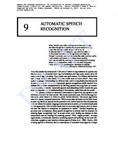
Figure 4.1: Histogram for pr : from 0.0 to 0.4 in 128 steps. Details: impostors at perplexity 20, Oct 1996 MFCC-based recognizer, OGI Names corpus, raw probabilities, frame-toword averaging, word models from Orator TTS, 16000 trials, nal test set. discussed in section 4.4.1. E�ective use of impostors is made di�cult by the fact that this is open-set rejection.
ANN-based Recognizer: Each experiment uses a recognizer to identify what phoneme
is being uttered at each point in time. The Oct 1996 MFCC-based recognizer is used in this experiment and most or all other experiments. It is described in section 4.1.2.
Word Models: word models from Orator TTS (described in section 4.6.2) are used in this experiment. Word models in general are described in section 4.6.
4.2.4 Results: Raw Score Histogram The results of these trials are shown by the histograms in Figure 4.1. (Section 4.8.2 gives details on histogram creation and smoothing.) The true scores have a median value of
4.2 Performing One Experiment
29
Total Verification Error 1.0
Error Rate
0.8
MVE=0.6396
0.6
Type I error Type II error total error
0.4 EER=0.3200 0.2 0.0 0
0.05
0.1
0.15 0.2 0.25 Raw Score
0.3
0.35
0.4
Figure 4.2: Various Error Rates for pr : from 0.0 to 0.4. Details: impostors at perplexity 20, Oct 1996 MFCC-based recognizer, OGI Names corpus, raw probabilities, frame-toword averaging, word models from Orator TTS, 16000 trials, nal test set. Type I error is rejection of truth. Type II error is acceptance of falsehood. 0.12 and the impostors have a median value of 0.06. It is clear to see that there is a substantial di�erence between the two distributions, and that the simple algorithm does distinguish to some extent between correct and impostor recognitions. The overlap seems rather large but improvements will be made in subsequent experiments. (The emphasis in this chapter is to identify the methodology.)
4.2.5 Total Veri cation Error Figure 4.2 presents the error rate for various raw score values. Three error rates are presented: Type I, Type II, and total (TVE). The Type I error rate (de ned for example in Spence, Cotton, Underwood, and Duncan 1992) is the proportion of true word scores that would be rejected at that threshold. It is also called the � error. The Type II error rate is the proportion of impostor word scores that would be accepted at that threshold.
4.2 Performing One Experiment
30
Table 4.3: Mean, Standard Deviation, and 95% Con dence Interval for the pr Algorithm. Details: impostors at perplexity 20, Oct 1996 MFCC-based recognizer, OGI Names corpus, frame-to-word averaging, word models from Orator TTS, 16000 trials, nal test set, equal error rates. Algorithm mean�sx� n 95% con d pr .3200�.0023 200 .3155{.3245 It is also called the error. The sum of these is the Total Veri cation Error (TVE). TVE dips and rises with a minimum veri cation error (MVE) of .6396 near 0.085. MVE is the minimum point on the Total Veri cation Error curve. In both gures (4.1 and 4.2) the better scores are toward the right. Scores to the right of a threshold would be accepted while those to the left of the threshold would be rejected. At one extreme (in this case a threshold of 0.0) all scores are accepted. The Type I error rate is 0.0, since no true recognitions are rejected. The Type II error rate is 1.0, since all imposters are accepted. At the other extreme (in this case a threshold of 1.0) all scores are rejected. The Type I error rate is 1.0 since all true recognitions are incorrectly rejected. The Type II error rate is 0.0 since all imposters are correctly rejected. Between these two extremes there is a raw-score threshold (say 0.085) at which the error rates are equal. This rate is .3200. That means that .3200 of the true recognitions would be incorrectly rejected, and .3200 of the impostor recognitions would be incorrectly accepted at that threshold. This is the Equal Error Rate (EER). EER is used as the primary decision statistic in this research, but some interesting alternatives are discussed in section 4.8.3.
4.2.6 EER Statistics Table 4.3 presents the estimated mean, standard deviation, and 95% con dence interval for algorithm pr . Each of the terms used in the table and caption is explained below.
mean�sx�: The mean is the mean equal error rate for the algorithm in question. It is
de ned as the equal error rate of the original raw scores before bootstrapping is performed.
4.2 Performing One Experiment
31
is the standard deviation of the mean, which is the square root of the variance of the bootstrap estimates. sx�
Bootstrap Iterations: The bootstrap procedure (described in section 4.8.5) is a sta-
tistical method for estimating the variance of quantities that may otherwise be hard to evaluate. Brie y the procedure involves treating the sample as though it were a population, and repeatedly drawing same-size samples from it (with replacement). The variance of these secondary (bootstrap) samples is an estimate of the true variance.
n: This is the number of bootstrap iterations. Each iteration produces an estimate of the mean. (This is not the number of trials performed.)
95% con d: The true EER is not known, and must be estimated by statistical means.
The estimate may also be wrong, but it is possible to state a range (a con dence interval) in which the truth is likely to lie. For the con dence interval tables, these ranges indicate that 95 times out of 100 the truth will lie within the range given. This is a central range, which means that half the errors will be on each side of the range. These central con dence intervals are computed by the standard-deviation method using Student's t distribution. See section 4.8.5 for more details.
impostors at perplexity 20: This is the perplexity used in these experiments. It is
the number of randomly selected word models from which the best was chosen to be the impostor. This is described in section 4.4.2.
Oct 1996 MFCC-based recognizer: This is the recognizer used in these experiments. It is described in section 4.1.2.
OGI Names corpus: This is the corpus is used in these experiments. It is described in section 4.5.1.
frame-to-word averaging: This is the method by which frame scores were accumulated
into word scores. In this case the word scores were computed directly by averaging the
4.3 Comparing Several Experiments
32
individual frame scores within the word. Other ways of accumulating the word score are presented in section 5.4.
word models from Orator TTS: Word models are generated using the Orator text-
to-speech system. It is described in section 4.6.2.
16000 trials: 16000 recognition trials (or some other number) are used to collect examples for scoring. This process is described in section 4.8.1. A larger number of trials generally results in a better estimate of the mean, as the standard deviation of the mean tends to decrease with the square root of the number of trials performed.
nal test set: This is the test set used in these experiments. Test sets are described in section 4.5.
4.3 Comparing Several Experiments How can comparison be made among several algorithms? The basic approach is to compare their equal error rates to identify the algorithm that performs best. To illustrate this comparison two additional algorithms are discussed and evaluated.
4.3.1 Hypothesis The hypothesis for comparisons is that one algorithm is signi cantly better than another algorithm at identifying errors. Statistically, the equal error rate of one will be signi cantly better than the equal error rate of the other.
4.3.2
pn :
normalized probabilities
The rst of these algorithms modi es the pr raw score by normalizing each frame so the scores sum to 1.0. These new scores are called pn for \probability normalized." The methodology is exactly as stated for the pr algorithm. The results (given in Table 4.4) show a solid decline from pr , indicating that something important has probably been lost or masked due to this normalization.
4.3 Comparing Several Experiments
33
Table 4.4: Mean, Standard Deviation, and 95% Con dence Intervals for Algorithms in the
pr Family. Details: impostors at perplexity 20, Oct 1996 MFCC-based recognizer, OGI
Names corpus, frame-to-word averaging, word models from Orator TTS, 16000 trials, nal test set, equal error rates. For more explanation see page 30. Algorithm
pr pn pn=(1 ; pn )
4.3.3
pn =(1 ; pn ):
mean�sx� n 95% con d .3200�.0023 200 .3155{.3245 .3421�.0023 200 .3376{.3466 .3621�.0024 200 .3573{.3669
likelihood ratio (odds)
The second of these algorithms uses a likelihood ratio or odds formulation. The likelihood ratio is de ned as the probability of truth divided by the probability of error. In this case the truth is represented by pr and error by the sum of all other ANN scores in the same n frame. This is mathematically equivalent to 1;p pn . Since it is easy to convert both ways between pn and pn =(1 ; pn ) no information is lost. However, the emphasis changes to favor frames with high likelihoods and discount frames with low ones. The same methodology is used. The results (given in Table 4.4) show a further decline from pn . The decline in performance must be due to the change in emphasis which has resulted in scores that do not accumulate as accurately.
4.3.4 Mean, Standard Deviation, and Con dence Intervals Table 4.4 presents the estimated mean, standard deviation, and 95% con dence interval for the three simple algorithms considered in this chapter.
4.3.5 Mileage Chart Table 4.5 presents a Mileage Chart for the three simple algorithms considered in this chapter. It is styled after the mileage charts often found on road maps, which give the distance in miles between cities. This mileage chart gives a statistical distance between algorithms, telling how rarely such a di�erence in performance would arise by chance. The caption information is described on page 30. Performance gures (mean�sx� ), algorithm names, and other information that varies from case to case is listed along the
4.3 Comparing Several Experiments
34
Table 4.5: Mileage Chart for Algorithms in the pr Family. Details: impostors at perplexity 20, Oct 1996 MFCC-based recognizer, OGI Names corpus, frame-to-word averaging, word models from Orator TTS, 16000 trials, nal test set, equal error rates.
�
.3200 .0023,
pr
9 .3421�.0023, pn 18 7 .3621�.0024, pn=(1 ; pn) main diagonal, best rst, starting in the upper left corner. The distance between two algorithms is shown at the intersection of their respective row and column. Low numbers indicate the di�erence could be due to chance. High numbers indicate the di�erence is signi cant. A distance of 0 means that even when no di�erence exists in the true means, these estimates will have such a di�erence by accident more than 1 time in 10. 1 means 1 in 10 or less (two-tailed � � :1). 2 means 1 in 100 or less (:001 < � � :01). n means between 1 chance in 10n and 1 chance in 10n+1 . Table 4.5 indicates that pr is better than pn since that is their order on the main diagonal. The 9 indicates that their di�erence could happen by chance only 1 time in 109 or less. Further, pr is better than pn =(1 ; pn ). 18 means the chance of getting such a di�erence by unlucky sampling is less than 1 in 1018. And pn is shown to be better than pn=(1 ; pn ) unless a 1 in 107 mistake occurred. It is normally safe to trust numbers greater than 2. Distance numbers are computed by taking the two-tailed � value based on the computed t score1 , and then reducing it by taking its logarithm to base 10.
4.3.6 EER Across Algorithms The mileage chart presents a large amount of information in a very compact format. For some pairs of algorithms a more detailed presentation may be appropriate. This is provided in the \EER Di�erences Across Algorithms" tables. Table 4.6 compares the Equal Error Rate between pairs of algorithms in the set considered in this chapter. For each line the algorithm on the left has a better (or equal) 1 t score tail area is computed using the public-domain algorithm 27 from \Applied Statistics, Volume 19, number 1."
4.4 Impostors and Perplexity
35
Table 4.6: Di�erences Across Selected Algorithms in the pr Family. Details: impostors at perplexity 20, Oct 1996 MFCC-based recognizer, OGI Names corpus, frame-to-word averaging, word models from Orator TTS, 16000 trials, nal test set, equal error rates. Better Algorithm EER�sx� pr .3200�.0023 pr .3200�.0023 n p .3421�.0023
Di�erence Worse di� t df � EER�sx� Algorithm 6% 6.85 398 .0000 .3421�.0023 pn n 12% 12.61 398 .0000 .3621�.0024 p =(1 ; pn ) 6% 5.98 398 .0000 .3621�.0024 pn =(1 ; pn )
EER. The percentage di�erence (improvement) over the algorithm on the right is shown, together with the statistical t score for such a di�erence, and the probability of getting that di�erence or more by random chance (two-tailed � level).
The Rest of the Chapter: The remaining sections of this chapter present issues al-
ready touched upon, but do so in more depth. These details were deferred until now to make the initial presentation easier to follow.
4.4 Impostors and Perplexity Closed-set means that the utterance is guaranteed to match one of the word models. With closed-set rejection, each word model can be considered in turn and if two word models both match well (e.g., \Doug" and \dog") this fact can be known and used. Open-set rejection is more di�cult. Say for example that the active vocabulary is \dog," \cat," and \bird." Say also that the actual utterance is \Doug." What should be done? Is it close enough to be called \dog"? Since one does not know which other words might be uttered, it is di�cult to decide just how similar the utterance must be to the word model. The problem is handled here by the creation of impostors based on a perplexity parameter.
4.4.1 Impostors For each utterance the true identity of the word is recorded by a trained human listener. Since there is only one true word for each utterance, scoring is straightforward. The scores
4.4 Impostors and Perplexity
36
of randomly selected true words provide an estimate of the frequency distribution of all true words. There are many di�culties surrounding the generation of impostors. Ideally they would mimic the distribution of real-world impostors. This is much more di�cult to know than for true words. It varies from task to task in ways that this research does not attempt to model. The approach taken here is to select impostors from the same corpus that provided the correct word. The actual creation of impostors is done by selecting several word models at random, together with one utterance wave le that does not match any of the word models. Viterbi search is used to identify the best-matching word model and it is declared to be \the" impostor for that utterance. It is scored as though it were a true word. For simplicity all incorrect utterances and word models are assumed to be equally likely. This is a fairly gross simpli cation, as some names are rather common and others quite rare. However, all algorithms are tested under the same assumption and it is expected that relative rankings would be stable across any reasonable variation in the frequency of particular names. (To prove this is true the algorithms are evaluated in section 5.1 with other corpora. The relative results appear to be stable.) Scores from true words and impostors must be distributed di�erently in order for con dence and rejection to be better than random chance. It is the job of the algorithm to create such scores.
4.4.2 Perplexity The term \perplexity" is used to refer to the number of word models from which the impostor was chosen. In a perplexity-20 setting, each impostor is the best match from a set of 20 word models drawn at random. As the perplexity increases, the goodness-of-match for the impostor also improves. With a large enough vocabulary it becomes almost certain to nd an impostor that scores as well or better than the true word model does.
4.5 Corpora
37
4.5 Corpora Corpora are collected bodies of recorded speech. The speech is encoded into wave les. For the present research, they also are required to have a word-level transcription, allowing evaluation of recognition results.
Telephone Speech: The research conducted has been directed towards telephone speech.
An important characteristic of telephone speech is reduced frequency bandwidth. Telephone speech is ltered to occupy the frequency spectrum from 300 Hz to 3400 Hz (more or less) and is typically sampled at 8000 Hz. Channel characteristics play a r^ole with telephone speech. The quality of transmission has improved with the use of digital signaling on switch-to-switch connections, but analog segments remain in the telephone network, especially in the \ rst-mile" wiring from the customer to the local switch. The corpora used in this research are actual telephone speech collected across the public telephone network in the US.
Two Extremes: The Names corpus presents a fairly di�cult recognition task, while
the PhoneBook corpus presents a fairly easy recognition task. Together these mark out interesting limits for the evaluation of con dence and rejection algorithms.
Partitioning to Train and Test: Each corpus is divided into several sets. Calls in the
training set are used to develop algorithms. Calls in the development test set are used to evaluate and compare algorithms, arriving at preliminary conclusions. Calls in the nal test set are \new" utterances never before seen by the system, and are used to verify the preliminary conclusions.
4.5.1 Names: OGI Names corpus The OGI Names Corpus (http://www.cse.ogi.edu/CSLU/corpora/names.html) is described on its web page as follows: \The : : : Names Corpus is a collection of rst and last name utterances. The utterances were taken from many other telephone speech data collections
4.5 Corpora
38
that have been completed at the CSLU, during which callers were asked to say their rst and last names, or asked to leave their name and address to receive an award coupon. Each le in the Names corpus has an orthographic transcription : : : ." Its internal documentation states: \There is a large variability in the spelling of English names. In the case of common names, plausible spellings were intuitive. However, for the rarer names, we transcribed using an orthography which resembled the pronunciation as closely as possible. We have not attempted to standardize the name spellings. Over the whole corpus there are about 10570 unique names. No standard spellings are used so names such as `kerri' and `kerry' will be counted as two separate tokens. The corpus consists of about 6.3 hours of speech." This corpus is further described in Cole, Noel, Burnett, Fanty, Lander, Oshika, and Sutton (1994) and Cole, Fanty, Noel, and Lander (1994). The current version (release 2) of the OGI Names corpus has 24 000 utterances distributed as follows: rstname 9727, lastname 11431, other1 151, other2 29, other3 2, other4 1, whole 2659.
Special Characteristics: The OGI Names corpus is relatively di�cult for recognition
and con dence. Following are some possible reasons. Utterances may be cut from running speech rather than being isolated pronouncements. Name spellings tend to be obscure and less-phonetic than other words, making phonetic-based recognition more error-prone. In addition, the utterances may be autographic (i.e., spoken by the owner of the name) which makes them idiosyncratic to the extent the person has developed a style for saying his or her name, also making phonetic-based recognition more error-prone. The average le length is 943 msec.
Training and Test: The corpus is divided into several sets. By convention at CSLU
(the Center for Spoken Language Understanding at Oregon Graduate Institute (OGI)) this division is made by call number. As each call arrives it is assigned a serial number. If the last digit is 0, 1, 2, 5, 6, or 7, the call is assigned to the training set. If the last digit is 3 or 8 the call is assigned to the development testing set. If the last digit is 4 or 9 the
4.5 Corpora
39
call is assigned to the nal testing set. From a total of 24000 utterances, there are 14380 utterances (60%) in the training set, 4854 utterances (20%) in the development test set, and 4766 utterances (20%) in the nal test set. All utterances in the same call are assumed to be by the same person. Each call is assumed to be by a di�erent person. There are known to be exceptions. The actual amount of duplication is unknown but believed to be inconsequential.
4.5.2 PhoneBook: NYNEX PhoneBook corpus As detailed in the PhoneBook Final Report (Pitrelli, Fong, and Leung 1995), \PhoneBook is a phonetically-rich, isolated-word, telephone-speech database : : : of American English word utterances incorporating all phonemes in as many segmental/stress contexts as are likely to produce co-articulatory variations, while also spanning a variety of talkers and telephone transmission characteristics. : : : The core section of PhoneBook consists of a total of 93,667 isolated-word utterances, totaling 23 hours of speech. This breaks down to 7979 distinct words, each said by an average of 11.7 talkers, with 1358 talkers each saying up to 75 words. All data were collected in 8-bit mu-law digital form directly from a T1 telephone line. Talkers were adult native speakers of American English chosen to be demographically representative of the U.S." The words were organized into about 100 word lists, and each list was read by about 15 talkers. Five words (\examiners," \hire," \hutchins," \sports," and \your") appear on more than one list. With the exception of the ve repeated words, there is no overlap between sets, either in the vocabulary words used or in the speakers themselves. This provides both speaker independence and vocabulary independence between the three sets.
Special Characteristics: The PhoneBook corpus is relatively easy for recognition and
con dence. Following are some possible reasons. Utterances are isolated pronouncements. The pronunciations are screened to avoid rare or surprising variations. A pronunciation dictionary (modi ed from the CMU dictionary) is included with the corpus. The apparent
4.6 Pronunciation and Word Modeling
40
randomness of the words themselves may cause the talker to enunciate them more carefully so as to avoid misrecognition as another word. The words were generated in a way that maximizes the phonological coverage of English, and guarantees that each word contains a unique phonological context not present in any of the other words. This unique context may make it easier to discriminate between correct and incorrect word models. The words also tend to be long because long words provide more phonological contexts. This tends to give more phonemes that will be wrong for an incorrect recognition. The average le length is 884 msec (about the same as OGI Names).
Training and Test: At CSLU the word lists are divided into a training set (50%), a
development test set (25%), and a nal test set (25%). AK68_M1O is a typical PhoneBook lename. Its second letter (e.g., K) is used to partition the corpus. Odd letters (A, C, E, G, I, K, M, O, Q, S, U, W, and Y) are assigned to the training set. The rst half of the even letters (B, D, F, H, J, and L) are assigned to the development test set. The remaining letters (N, P, R, T, V, X, and Z) are assigned to the nal test set.
4.5.3 Corrections No wave les were eliminated from either corpus. Transcriptions were regularized in an automated way to facilitate the generation or lookup of pronunciation models. This involved removal of informative markings such as
(indicates the presence of breath noise) and hypothesized portions of words (jonath[an] indicates the end of this name was cut o� but believed to be as shown).
4.6 Pronunciation and Word Modeling For each recognition attempt the Viterbi search algorithm aligns all available word models against the ANN outputs from the utterance. The model that scores best is declared winner. Word models that are not provided with the corpus must be derived in some other way. Recognition (described more fully in section 4.7) is done by matching ANN outputs to a word model. The word model is speci ed as a list of phonemes. The Worldbet phoneme
4.6 Pronunciation and Word Modeling
41
set (Table 4.7) is used to express word models and to identify phonemes. Using this scheme a word model can be constructed based on the pronunciation of the word. For example, the word \yes" can be modeled as /j E s/ and the word \no" can be modeled as /n oU/. When word models are needed they are retrieved from a dictionary or generated using a Text-to-Speech (TTS) algorithm. Available public-domain or free dictionaries include the CMU dictionary and the Moby dictionary. Available TTS algorithms include Orator from Bellcore, DECtalk from Digital Equipment Corporation, and Rsynth from the University of Cambridge (UK). Other dictionaries and TTS programs exist, and a number of them are listed in the FAQ (frequently asked questions) of the comp.speech newsgroup. Alternately pronunciations could be gathered from phonetically labeled corpora such as the OGI Stories corpus, and with practice ordinary people could create word models just as they can now spell, but these approaches are not pursued in this research. Phonetic word models must be further modi ed to produce ANN-speci c word models that identify the exact sequence of ANN outputs needed for that word. For instance, the transition /j E/ may be modeled as \ rst half of j after silence" followed by \second half of j leading into E" followed by \ rst third of E starting after j" followed by \central third of E." Each of these context-dependent phonemes would correspond to some speci c output of the ANN. These ANN outputs are presented in tables 4.1 and 4.2.
4.6.1 Worldbet Symbols Table 4.7 shows Worldbet symbols used to specify word models.
4.6.2 Orator: word models from Orator TTS The web page http://www.bellcore.com/ORATOR/ presents the following information (June 1997). \Bellcore's ORATOR(tm) Speech Synthesizer provides the tools for high quality, highly accurate telephone access to database-driven information services through the process of text-to-speech synthesis. ORATOR's rst commercial use is a popular reverse-telephone-directory service, currently available in Illinois. \ORATOR's Features Include: * Highest accuracy for name pronunciation available for American people, places, and businesses. * A high level of speech intelligibility -
4.6 Pronunciation and Word Modeling
42
Table 4.7: Worldbet Symbols: The Worldbet symbols are used to form word models. OGI symbols are also given because they are familiar to many researchers. The samples are common English words that exhibit the speci ed phoneme. Worldbet OGI Sample Worldbet OGI Sample Worldbet OGI Sample i: iy beet iU few s s sign I ih bit aU aw about S sh assure E eh bet oU ow boat s s sign @ ae bat ph p pan S sh assure & ax above th t tan h hh hope u uw boot kh k can v v vine U uh book b b ban D dh thy ^ ah above d d dan z z resign > ao caught g g gander Z zh azure A aa father m m me tS ch church 3r er bird n n knee dZ jh judge &r axr butter N ng sing l l lent ei ey bay d_( dx rider 9r r rent aI ay bye f f fine j y yes >i oy boy T th thigh w w went uc unvoiced closure (before ph, th, kh, tS) .br breath noise vc voiced closure (before b, d, g, and dZ) .pau pause or silence resulting in clear and natural sounding speech. * Excellent acronym pronunciation. * Words spelled out upon request, with human-like letter grouping. * Flexible, powerful facilities for customized pronunciation and intonation. * Ports to a variety of platforms." Orator is used with each name to produce a word model for that name. The word model consists of the sequence of phonemes that would have been uttered by Orator if it were attempting to pronounce that name.
4.6.3 CMU: word models from CMU dictionary The CMU dictionary is described on its web page as follows (June 1997): \The Carnegie Mellon University Pronouncing Dictionary is a machine-readable pronunciation dictionary for North American English that contains over 100,000 words and their transcriptions. This format is particularly useful for speech recognition and synthesis, as it has mappings from words to their pronunciations in the given phoneme set. The current phoneme set
4.6 Pronunciation and Word Modeling
43
contains 39 phonemes..." It is also cited in the comp.speech FAQ. A version of the CMU dictionary is provided with the NYNEX PhoneBook corpus. Word models are determined by dictionary lookup for the words in this corpus.
4.6.4 Wordspotting Grammars Before and after each word, a ller model is required by the grammar. It is sometimes referred to as the \any model" because it matches anything. It models the context around the word in question. If the utterance were \I'm John (breath)" and the word model were \dZ A n" the ller model would need to account for the frames belonging to the preceding \I'm" and to the following breath noise. The grammar requires the rst frame of the utterance to belong to the leading ller model, and the last frame to belong to the trailing ller model. More frames can be assigned to the ller models by the Viterbi search if it improves the overall word score. In general, grammars are composed of word models, just as word models are composed of phonemes. Words are modeled as formal regular expressions, and grammars as formal context-free grammars. Grammars are particularly useful for specifying recognizers of connected-digit strings, dates, times, or other multi-word objects where repetition or branching are important within the model. In the context of the current research, grammars are used only to support wordspotting.
Filler Modeling: A typical wordspotting grammar is
word .
This model divides the utterance into three parts, and uses an arti cial phoneme in the scoring process. The phoneme is de ned as having the same neural network output value as the median of the top n other phonemes (typically n defaults 30 or 50) or of the silence phoneme, whichever scores better. (The median approach is based on HMM work by Bourlard et al. 1994). In each frame, the phoneme with (counting from one) the 16th highest value (30=2 + 1) is identi ed, and the value is copied to become the value of the phoneme. If silence scores better, then it is copied instead. is used to account for phonemes outside the target word, and thus provides wordspotting capability.
4.7 Recognition by Viterbi Alignment
44
4.7 Recognition by Viterbi Alignment The recognizer operates by aligning the actual utterance (digitally recorded) with a computer model of the target word. This alignment process creates (as a side e�ect) a score that gives the relative likelihood that the word model is correct for that utterance. This recognition score (also called the Viterbi score) is computed for each of the word models, and the model with the best score is selected.
4.7.1 Frames and Words Each utterance is divided into frames of xed length. This length is 10 msec. Researchers use a variety of frame sizes. The 10 msec length is inherited from the recognizer and is taken as a given. It is not optimized in any way for this con dence and rejection research. Viterbi search is the process by which each frame is assigned to one of the parts of the word model. An example may help. Say an utterance is \yes" and has a duration of 0.90 seconds. The word model is \j E s" (word models and the phonetic alphabet are explained more fully in section 4.6) and the grammar is \any yes any." At 10 msec per frame there are 90 frames in this utterance. They are numbered from 0 to 89. By Viterbi search, frames 0{7 are assigned to the ller model, frames 8{11 are assigned to the phoneme \j," frames 12{26 to the phoneme \E," and frames 27{44 to the phoneme \s." The remaining frames, 45{89, are again assigned to the ller model. Each of these ve parts is called a segment.
4.7.2 ANN Probability Pro les The recognizer ANN is employed to estimate a score pr for each frame of the utterance. This score is computed for all possible phonemes, giving not just a single score but an entire pro le of scores at each moment in time. In the example above, the Viterbi search algorithm uses the ANN scores from \j" and \E" in frame 11 to assign that frame to the \j" segment. Note that the probability for \j" must be higher than the probability for \E" or else the frame would have been assigned to the \E" segment instead.2 These 2 This is a simpli cation. Segment duration and other constraints can also a�ect the score and segmen-
tation assignments. There is a penalty applied for segments that are too short or too long compared to
4.8 Statistical Issues
45
probabilities approximate the true a posteriori probability of the phoneme classi cation given the acoustic evidence.
4.8 Statistical Issues 4.8.1 Sampling and Trials A randomized sample of utterances and word models is drawn from the corpus. The sample size n (number of trials) is chosen to reduce the variance of performance statistics so that measured di�erences will be statistically valid. In each of the n trials an utterance is selected at random. The word model is generated for the correct word, recognition is performed, and a raw word score is computed by averaging the frame scores. An impostor (section 4.4.1) is also generated and scored. The true word score and the impostor word score are kept. Eventually there are n of each score. Note that it does not matter whether the utterance is chosen rst or the impostor candidates are chosen rst. In any case, the impostor score represents an out-of-vocabulary speech recognition event, where the candidates represent the active vocabulary and the utterance is out-of-vocabulary with respect to that set.
4.8.2 Histogram Creation Histograms such as those in Figure 4.1 are created in the following manner. All raw scores are reviewed and the highest and lowest are identi ed. The interval between them is divided into n bins. Each raw score is examined and the appropriate bin count is incremented. For the nal histogram, smoothing is performed as follows. The count in each bin is reallocated with 25% going to the bin on the left, 50% to the original bin, and 25% to the bin on the right. This is done simultaneously for all bins. The presentation of the histogram is done by connecting center-points of each bin. the proper duration for a segment of that type. For instance, if the proper duration is given as 30 to 200 msec, and the modeled duration is 250 msec, there will be 50 msec of too-long penalty applied to the word score. Similarly if the modeled duration is only 10 msec there will be 20 msec of too-short penalty applied to the word score.
4.8 Statistical Issues
46
Receiver Operating Characteristics
1 - Type I Error Rate
1.0 0.8
MVE ROC EER
0.6 0.4 0.2 FOM is area under ROC 0.0 0.0
0.2
0.4 0.6 Type II Error Rate
0.8
1.0
Figure 4.3: Annotated ROC Curve: The ROC arches from (0,0) to (1,1), showing the tradeo� between the two types of errors. The MVE is the point of tangency on a 45� line tangent to the ROC. The EER is the point of intersection on a 45� line from (0,1) to (1,0). The FOM is the area under the ROC curve. This method is chosen instead of the more common drawing of square corners for each bin because the squared histogram proved much more di�cult to read, especially in areas where two lines were close to each other. For some histograms the highest and lowest scores were not used, but a top and bottom of the range was chosen to better focus on the region of interest. This was helpful in cases where outliers caused the histogram to be compressed, thus obscuring interesting details.
4.8.3 The ROC Curve The receiver operating characteristic (ROC) curve shown in Figure 4.3 arches from (0,0) to (1,1), showing the tradeo� between the Type I and Type II errors. The minimum veri cation error (MVE) is at the point of tangency on a 45� line that is tangent to the ROC. The equal error rate (EER) is at the point of intersection on a 45� line from (0,1)
4.8 Statistical Issues
47
to (1,0). The gure of merit (FOM) is the area under the ROC curve. Because the axes are error rates the presentation is normalized which makes it possible to visually compare two ROC curves to identify the better performance. Each raw score corresponds to some point on the curve, but raw scores are not presented explicitly. Geometric characteristics of the ROC curve are used in comparing algorithms. The aspect used throughout this thesis is the equal error rate (EER). The MVE and FOM serve as alternatives to the EER in the comparison of algorithms. In-depth discussion of ROC curves and likelihood ratios can be found in chapter 2 of Van Trees (1967).
4.8.4 Alternatives to EER: MVE and FOM Figure of Merit: The gure of merit (FOM) is de ned as the average accuracy across
all Type I or Type II error rates. More simply this is the area under the ROC curve. Ideal performance produces a score of 1.0. As such it re ects total performance and not just the performance at one speci c threshold. Random performance produces a score of .5. The residual error rate is 1;FOM.
Minimum Veri cation Error: The MVE generally occurs at or near the EER and is
therefore approximately twice as great. The optimal decision point to minimize overall error depends on the relative frequency of impostor recognitions. When impostors occur half of the time the optimal point is the MVE. It lies on the equal-cost line which is ec = T1 + T2 , where ec is chosen to make the line tangent to the ROC.
Minimum Cost Point: The optimal decision point to minimize overall cost depends
on the relative costs of Type I and II errors. This varies by task and is beyond the scope of the current research. However, a variation in costs also has a geometric interpretation on the ROC curve. If the cost of a Type I error is $5 and the cost of a Type II error is $10, the equal-cost line will be ec = 5T1 + 10T2, where ec is chosen to make the line tangent to the ROC.
4.8 Statistical Issues
48
4.8.5 Bootstrap Parameter Estimation In order to evaluate the stability of computed performance rates it is helpful to estimate the variance of the comparison metric. Because of the way the EER, MVE, and FOM are constructed it is di�cult to give a closed-form speci cation of the variance. Instead statistical bootstrapping (Efron and Tibshirani 1993) is used to estimate variances and evaluate the di�erence in performance of two algorithms. Bootstrap parameter estimation is performed as follows. Given a collection of n samples from which a single summary is computed (e.g., 16000 recognitions from which an EER is computed), select n samples from among the original n samples with replacement. Then compute the summary value again. Repeat this process a number of times (e.g., 200 times). The summary values thus computed can be examined to determine their distribution. In particular the summary values can be used to estimate their variance or a Monte Carlo con dence interval. In the current research, central con dence intervals are computed by the standarddeviation method using Student's t distribution. These intervals are known to be inaccurate to the extent the distributions are skewed, but as illustrated in Figure 4.4 it is seems reasonable to believe the distributions are approximately normal. Further, the signi cance numbers reported in this thesis tend to extremes. They are either inconclusive (� is large) or highly conclusive (� is almost zero). The Monte Carlo con dence-interval method is not used because the distributions are believed to be approximately normal and the added cost of computing enough bootstrap scores was prohibitive.
4.8 Statistical Issues
49
Bootstrap EER Distribution
Frequency
20
15
10
5
0 0.31
0.315
0.32 0.325 Equal Error Rate
0.33
Figure 4.4: Bootstrap EER distribution for pr : 200 bootstrap samples plotted from 0.31 to 0.33 in 32 steps. Details: impostors at perplexity 20, Oct 1996 MFCC-based recognizer, OGI Names corpus, raw probabilities, frame-to-word averaging, word models from Orator TTS, 16000 trials, nal test set.
Chapter 5 Vocabulary-Independent Experiments Each section in this chapter addresses a particular set of experiments, presenting the motivations, results, and conclusions. The general methodology is described in chapter 4 and is not repeated here except to point out variations.
5.1 Di�erent Corpora Ideally the particular choice of a speech recognition corpus would not have any e�ect upon the ultimate evaluation of con dence or choice of thresholds for rejection. As much as possible the goodness of a particular raw score must be independent of the corpus from which it was drawn. One corpus may contain utterances that are di�cult to recognize, due to recording conditions or to the nature of the utterances themselves. Another corpus may contain utterances that are enunciated more clearly and recorded under favorable circumstances. Among the best con dence and rejection algorithms, the ranking should not depend upon the choice of corpus. The two experiments in this section will determine whether the results from sections 4.2 and 4.3 were a�ected by the choice of the OGI Names corpus to perform the experiments. Names presents a relatively di�cult task (see section 4.5.1). The rst experiment in this section looks at the NYNEX PhoneBook corpus, and the second looks at an equal mix of OGI Names corpus and NYNEX PhoneBook corpus. It is concluded that the Mixed corpus is an appropriate base upon which to compare algorithms.
50
5.1 Di�erent Corpora
51
Histogram Variation by Corpus 700 600 Impostor PhoneBook Impostor Names
Frequency
500 400 300
True PhoneBook True Names
200 100 0 0.0
0.1
0.2 0.3 Raw Score
0.4
0.5
Figure 5.1: Distribution variation across Names and PhoneBook for Algorithm pr . Trues show a large change in distribution between corpora. Details: impostors at perplexity 20, Oct 1996 MFCC-based recognizer, frame-to-word averaging, 16000 trials, nal test set, equal error rates. OGI Names corpus uses word models from Orator TTS. NYNEX PhoneBook corpus uses word models from CMU dictionary.
5.1.1 An Easier Corpus The NYNEX PhoneBook corpus (see 4.5.2) provides a fresh perspective. This corpus presents a relatively easy recognition task with utterances that are enunciated more clearly and recorded under more favorable circumstances than the OGI Names corpus.
Hypothesis: When experiments are rerun using the NYNEX PhoneBook corpus, the absolute results may vary but the relative results (one algorithm versus another) will be the same.
Results: Figure 5.1 shows a histogram of scores from the pr algorithm on Names and
5.1 Di�erent Corpora
52
Table 5.1: Di�erences Across Corpora for Algorithms in the pr Family. Details: impostors at perplexity 20, Oct 1996 MFCC-based recognizer, frame-to-word averaging, 16000 trials, nal test set, equal error rates. OGI Names corpus uses word models from Orator TTS. NYNEX PhoneBook corpus uses word models from CMU dictionary. PhoneBook Algorithm EER�sx� pr .2216�.0021 pn .2121�.0020 pn=(1 ; pn ) .2453�.0020
di� 31% 38% 32%
Di�erence Names t df � EER�sx� Algorithm 31.60 398 .0000 .3200�.0023 pr 43.31 398 .0000 .3421�.0023 pn n 37.10 398 .0000 .3621�.0024 p =(1 ; pn )
PhoneBook. The impostor curves do not vary much, but the true curves do vary substantially. The PhoneBook corpus gives much better true scores. Does this translate into a better equal error rate? Table 5.1 shows that performance on PhoneBook is 31% to 38% better than performance on Names by these algorithms. This indicates that PhoneBook is substantially easier to con rm or reject than Names. Table 5.2 shows that the relative results (one algorithm versus another) are not the same: pr and pn swap positions in the line-up, although both beat pn =(1 ; pn ). This shows that the best-scoring algorithm may vary by corpus. Clearly there is some risk in doing all evaluations across just one corpus.
5.1.2 An Averaged Corpus The relative performances of pr and pn are a�ected by the evaluation corpus used. Judging from the histograms the raw scores are compatible across corpora because the distributions almost coincide. A linear combination of the two corpora might serve better than either one alone. An equal mix will be examined.
Design: For this no new recognitions are performed. Instead the raw scores from Names
and PhoneBook are combined into a single list from which overall performance gures are determined. This is equivalent to doing class-based recognitions where the separate corpora each represent a large class and the recognition is constrained to be within that class but the rejection thresholds are controlled globally. The results may have been
5.1 Di�erent Corpora
53
Table 5.2: Corpus Di�erences Change Algorithm Rankings in the pr Family. Note that pr and pn change positions in the rankings. Details: impostors at perplexity 20, Oct 1996 MFCC-based recognizer, frame-to-word averaging, 16000 trials, nal test set, equal error rates. For more explanation see page 33. NYNEX PhoneBook corpus using word models from CMU dictionary
�
.2121 .0020,
pn
2 .2216�.0021, pr 17 11 .2453�.0020, pn=(1 ; pn) equal mix of OGI Names corpus and NYNEX PhoneBook corpus
�
.2755 .0014,
pr
2 .2814�.0015, pn 20 16 .3063�.0015, pn=(1 ; pn) OGI Names corpus using word models from Orator TTS
�
.3200 .0023,
pr
9 .3421�.0023, pn 18 7 .3621�.0024, pn=(1 ; pn) di�erent if the two corpora were mixed at recognition time because a di�erent set of impostors might have been chosen.
5.1.3 Conclusions Table 5.2 shows that the NYNEX PhoneBook corpus performs much better than the equal mix of OGI Names corpus and NYNEX PhoneBook corpus, which in turn performs much better than the OGI Names corpus. This shows that the rankings of algorithms one against another can change signi cantly based upon the corpus with which evaluations are done. (This may be an accident of the poor rejection capabilities of the algorithms viewed thus far.) Compared to true performance in the eld using real vocabularies, Names is believed to be too pessimistic and PhoneBook too optimistic. The combined corpus may more closely represent the actual recognition conditions that will prevail beyond the laboratory. It is not clear how this conjecture might be tested, so it will taken as an assumption.
Combined performance is used hereafter for comparison among algorithms
5.2 On-Line Garbage Modeling
54
because it is believed to be closer to expected real-world performance. Although some other linear combination of the two corpora is probably even better, it is not clear how to select the best combination. Therefore an equal mix (same amount from each) combination has been used. The performance of pr (.2755�.0014) is the best thus far.
5.2 On-Line Garbage Modeling It is useful to compare rejection performance with existing methods. CSLU has an existing rejection mechanism installed in its CSLUsh toolkit and in CSLUrp, the CSLU Rapid Prototyper. The rejection system is based upon research by Boite, Bourlard, D'hoore, and Haesen (1993) using HMMs and has been in use at CSLU for several years. In the discussion that follows, two word models will be considered. One is called the \target" word model. It represents a real word that is being evaluated for acceptance or rejection. It is scored by the recognizer and its Viterbi score becomes the \target word score." The other is called the garbage word model. This is an arti cial word composed of a sequence of garbage phonemes which are created similarly to the any model discussed in section 4.6.4. The garbage phoneme is de ned as having the same neural network output value as the median of the top n other phonemes (typically n defaults to 22). This is called the garbage median rank or garbage rank. (Median rank / 2 + 1 = rank.) In each frame, the phoneme with the 12th highest value is identi ed, and its value is copied to become the value of the garbage phoneme. Acceptance or rejection of the target word is based upon its whole-word Viterbi score, which includes all frames in the utterance. Speci cally the frames that map to the any model (see section 4.6.4) are included in the score. Also since the score is made by adding the logarithms of the frame scores across the whole word and each frame score is a probability (i.e., usually less than 1.0) the scores tend to become more and more negative for longer and longer words. To create a level playing eld for rejection decisions, the garbage score is computed in the same way as the target word score, using the same number of frames. Then
5.2 On-Line Garbage Modeling
55
if the resulting target score is better than the garbage score the recognition is accepted. Otherwise it is rejected. For example, if the garbage median rank is 22, then the utterance will receive a garbage score based upon median rank 22. This utterance-speci c score is the threshold for acceptance or rejection of any particular target word score for that utterance. Adjustment of the rejection rate is achieved by changing the garbage median rank. To compare this approach to others by using equal error rates it is necessary to convert each target word score to a common base. The most accurate way to do this is to compute for each target word the \garbage" median rank at which the word would be at the threshold between acceptance and rejection. This is called the \target" median rank. These estimated target median ranks are the unit of comparison across various utterances and target word models.
5.2.1 Estimating the Target Median Rank One could compute the garbage score for all possible garbage median ranks, and then take the two scores closest to the target word score. Between these a simple linear interpolation will result in an accurate estimated target median rank. (Alternately the closer, higher, or lower garbage median score could have been used. This would have resulted in quantization error and a loss of resolution, so it was not done.) Because computing several hundred garbage scores seems like overkill, the actual plan is to select a smaller number of ranks and to interpolate from them. These chosen ranks are called \knot points" because they form the vertices along a piecewise linear curve that stretches from garbage median rank zero to garbage median rank 1000 (depending upon the number of ANN outputs in the recognizer). I.e., they are the points at which the linear interpolation segments are tied together. The two knot-point garbage scores closest to the Viterbi score of the target word are used in linear interpolation (or extrapolation) to estimate the equivalent garbage rank, which is the threshold at which the word score would equal the garbage score. The piecewise linear model may not perform as well as a tted smooth curve might, but it is monotonic and relatively easy to compute. Since all scores are derived in the same way the piecewise nature is not expected to have a large e�ect upon the nal results.
5.2 On-Line Garbage Modeling
56
Table 5.3: Mean, Standard Deviation, and 95% Con dence Intervals for Algorithms in the g(a,b,c...) Family. Notice that performance is nearly identical for all cases. Details: impostors at perplexity 20, Oct 1996 MFCC-based recognizer, equal mix of OGI Names corpus and NYNEX PhoneBook corpus, whole-utterance on-line garbage scoring, word models depending on corpus, 32000 trials, nal test set, equal error rates. For more explanation see page 30. Algorithm g(4,16) g(0,4,16) g(0,10) g(0,2,4,8...) g(0,10,20...) g(0,2,4,6...)
mean�sx� .1554�.0013 .1554�.0013 .1555�.0014 .1556�.0014 .1557�.0014 .1557�.0014
n 50 50 50 50 50 50
95% con d .1528{.1580 .1528{.1580 .1527{.1583 .1528{.1585 .1530{.1585 .1529{.1586
To speci cally explore the sensitivity of this approach in terms of the \knot-points" at which the piecewise linear model is constructed, a variety of knot-point sets is examined. It is shown that the performance is not sensitive to the choice of points. That is, di�erent point sets yield the same rejection performance.
5.2.2 Initial Knot-point Experiments The following experiments were performed.
g(0,2,4,6...): on-line garbage piecewise linear interpolation with knot-points at 0, 2, 4, 6, 8, 10, 14, 18, 22, 30, and 50: The sledge-hammer approach is to compute
the garbage score for all possible median values. Due to the way the median value is mapped to an actual rank (right-shift by one) only even numbers need be tried. For each utterance, a Viterbi score is computed using a garbage model at each of the following median ranks: 0, 2, 4, 6, 8, 10, 14, 18, 22, 30, and 50. By observation it was discovered that most wrong scores are less than median rank 50. A histogram is shown in Figure 5.2. Performance is shown in Table 5.3 to be .1557�.0014.
5.2 On-Line Garbage Modeling
57
true 1 impostor 1 true 2 impostor 2 true 3 impostor 3
800 700 600 500 400 300 200 100 0 -5
0
5
10
15
20
25
30
35
40
Figure 5.2: Histogram of Algorithms, 1: g(0,2,4,8...); 2: g(0,10,20...); 3: g(0,2,4,6...). Notice that the histograms are nearly coincident for all three cases. Details: impostors at perplexity 20, Oct 1996 MFCC-based recognizer, equal mix of OGI Names corpus and NYNEX PhoneBook corpus, whole-utterance on-line garbage scoring, word models depending on corpus, 32000 trials, nal test set, equal error rates.
g(0,2,4,8...): on-line garbage piecewise linear interpolation with knot-points at 0, 2, 4, 8, 16, 32, and 64: This next selection of knot points is exponentially spaced
across the region where scores are expected to fall. For each utterance, a Viterbi score is computed using a garbage model at each of the following median ranks: 0, 2, 4, 8, 16, 32, and 64. A histogram is shown in Figure 5.2. Performance is shown in Table 5.3 to be .1556�.0014. This spacing seems to improve the accuracy slightly, but the di�erence is not statistically signi cant.
g(0,10,20...): on-line garbage piecewise linear interpolation with knot-points at 0, 10, 20, 30, 40, and 50: This selection of knot points is spaced equally (rather than exponentially) across the region where scores are expected to fall. For each utterance, a Viterbi score is computed using a garbage model at each of the following median ranks:
5.2 On-Line Garbage Modeling
58
0, 10, 20, 30, 40, and 50. A histogram is shown in Figure 5.2. Performance is shown in Table 5.3 to be .1557�.0014.
5.2.3 Dramatically Fewer Knot Points None of the preceding knot-point sets varied much in its nal performance result. A much smaller number of knot points may a�ect performance. It is not clear a priori whether the performance will be better or worse, as fewer points cannot follow the data as well, but more points may be over tting. And ultimately it may not be statistically signi cant either way.
g(0,4,16): on-line garbage piecewise linear interpolation with knot-points at 0, 4, and 16: This selection of three knot points is spaced exponentially across the region
where most scores are expected to fall. For each utterance, a Viterbi score is computed using a garbage model at each of the following median ranks: 0, 4, and 16. The histograms in Figure 5.3 are much di�erent from those in Figure 5.2, which shows that the choice of knot points has a big in uence on the eventual raw scores. However the performance, shown in Table 5.3 to be .1554�.0013, has not changed signi cantly.
g(4,16): on-line garbage linear interpolation with knot-points at 4 and 16:
This selection of two knot points is spaced exponentially across the region where most scores are expected to fall. For each utterance, a Viterbi score is computed using a garbage model at each of the following median ranks: 4 and 16. A histogram is shown in Figure 5.3. Performance is shown in Table 5.3 to be .1554�.0013.
g(0,10): on-line garbage linear interpolation with knot-points at 0 and 10:
This selection of two knot points is spaced linearly across the region where most true scores are expected to fall. 10 is near the dividing point between trues and impostors. For each utterance, a Viterbi score is computed using a garbage model at each of the following median ranks: 0 and 10. A histogram is shown in Figure 5.3. Performance is shown in Table 5.3 to be .1555�.0014. The apparent slight loss in performance might be attributable to using 0 instead of 4 as the rst knot-point.
5.2 On-Line Garbage Modeling
59
900
true 1 impostor 1 true 2 impostor 2 true 3 impostor 3
800 700 600 500 400 300 200 100 0 -10
-5
0
5
10
15
20
25
30
35
40
Figure 5.3: Histogram of Algorithms, 1: g(4,16); 2: g(0,4,16); 3: g(0,10). Notice that the histograms are much di�erent from those in Figure 5.2, which shows that the choice of knot points has a big in uence on the eventual raw scores. However the performance does not change signi cantly. Details: impostors at perplexity 20, Oct 1996 MFCC-based recognizer, equal mix of OGI Names corpus and NYNEX PhoneBook corpus, wholeutterance on-line garbage scoring, word models depending on corpus, 32000 trials, nal test set, equal error rates.
5.2.4 Conclusions The selection of knot points does not seem to a�ect the accuracy of the on-line garbage modeling technique. Table 5.4 tells the story. None of the di�erences is signi cant. In fact, each of the di�erences has better than 8 chances in 10 of occurring naturally even if no actual di�erence exists. Because it is impossible to tell apart these performances based upon equal error rate alone, g(4,16) is designated as the representative of this group based upon its simplicity of implementation, using only a single line to remap any Viterbi score into its estimated target median rank. The on-line garbage approach of g(4,16) achieves a performance of .1554�.0013, which is dramatically better than the performance of pr (.2755�.0014). This is probably due to
5.3 Log Averages
60
Table 5.4: Mileage Chart for Algorithms in the g(a,b,c...) Family. Notice that performance is nearly identical for all cases. Details: impostors at perplexity 20, Oct 1996 MFCC-based recognizer, equal mix of OGI Names corpus and NYNEX PhoneBook corpus, wholeutterance on-line garbage scoring, word models depending on corpus, 32000 trials, nal test set, equal error rates. For more explanation see page 33.
�
.1554 .0013, g(4,16)
0 0 0 0 0
� 0 .1555�.0014, g(0,10) 0 0 .1556�.0014, g(0,2,4,8...) 0 0 0 .1557�.0014, g(0,10,20...) 0 0 0 0 .1557�.0014, g(0,2,4,6...) .1554 .0013, g(0,4,16)
the summing of logarithms in computing the recognition score, as opposed to the simpleminded averaging of raw probabilities. Section 5.3 looks into this question.
5.3 Log Averages The three simple algorithms presented in chapter 4 and in section 5.1 averaged probabilities directly. The impostor histograms in Figure 5.1 are sharply skewed, and the true histograms are somewhat skewed also. A logarithmic transformation may render curves that are more normal. Independent probabilities are always combined by multiplication to create joint probabilities, which suggests averaging in the logarithm domain. This type of averaging is also called geometric averaging. Because positive numbers are more convenient1 for computation and logarithms of probabilities are not positive, the minus logarithm will be used. The simple algorithms from chapter 4 will each be modi ed by taking the minus logarithm of the probability for the frame score. (Gillick, Ito, and Young (1997) refer to ; log(pn=(1 ; pn )) as the \logit" or \loglikelihood" function.) This is shown to improve performance dramatically and will become a standard operation on probability-like frame scores. 1 e.g., for taking another log, raising to a power, or geometric averaging of various types.
5.3 Log Averages
61
Table 5.5: Mileage Chart for Algorithms in the log(pr ) Family Details: impostors at perplexity 20, Oct 1996 MFCC-based recognizer, equal mix of OGI Names corpus and NYNEX PhoneBook corpus, frame-to-word averaging, word models depending on corpus, 32000 trials, nal test set, equal error rates. For more explanation see page 33.
�
; log(pr ) .2110�.0014, ; log(pn ) 0 .2135�.0015, ; log(pn=(1 ; pn)) 32 31 .2755�.0014, pr 33 32 2 .2814�.0015, pn 39 38 20 16 .3063�.0015, pn=(1 ; pn)
.1639 .0012,
28 28 43 43 47
Hypothesis: When experiments ; log(pr ), ; log(pn), and ; log(pn=(1 ; pn)) are run,
the histograms will be more normal and the performance will improve in comparison to pr , pn , and pn =(1 ; pn ). Because they are so di�erent from each other, no hypothesis is made about the comparison of ; log(pr ) with the g(a,b,c...) algorithms.
Results: Table 5.5 shows that ; log(pr) is clearly ahead of the other algorithms, and that ; log(pn ) and ; log(pn =(1 ; pn )) are practically equal. It also shows that taking the logarithms of probabilities has produced a substantial improvement in rejection performance. The histograms in Figure 5.4 show the raw scores the three algorithms. The curves are much more normal in shape than those in Figure 5.1. Notice that ; log(pn ) and ; log(pn=(1 ; pn)) are very nearly equal. Transformation to the log domain has washed out most of the di�erences between normalized probability and odds. ; log(pr ) has higher variance but is much better separated than the other two. The normalized probabilies reduce the variance but increase the overlap between trues and impostors. The performance of ; log(pr ) (.1639�.0012) falls 5% behind the equal error rate of g(4,16) (.1554�.0013), the top whole-word on-line garbage model (t = 4:82, � � 10;5). The performance of g(a,b,c...) algorithms is hurt by the use of the utterance frames before and after those in the word model. That is, the score is based upon the entire
5.3 Log Averages
62
Histogram Variation for log(p) Algorithms 3000
True log(pn) True log(odds) True log(pr)
Frequency
2500 2000
Impostor log(pn) Impostor log(odds) Impostor log(pr)
1500 1000 500 0 0
2
4 6 Raw Score
8
10
Figure 5.4: Distribution Variation for Algorithms in the log(pr ) Family. log(pn) is ; log(pn); log(odds) is ; log(pn=(1 ; pn)); log(pr) is ; log(pr). Notice that pn and pn =(1 ; pn) are nearly identical, and that pr is substantially better. Details: impostors at perplexity 20, Oct 1996 MFCC-based recognizer, equal mix of OGI Names corpus and NYNEX PhoneBook corpus, frame-to-word averaging, word models depending on corpus, 32000 trials, nal test set, equal error rates. utterance, including frames that are assigned to the any model before and after the word. It does not seem reasonable that the any model portions of on-line garbage are helping. At best the any model portions would provide random noise into the measurements. It must be something else. The other aspect is the normalization that is taking place in the g(a,b,c...) algorithms by using garbage phoneme scores as a point of comparison. This is examined further in section 5.5.
5.4 Segmental Averaging
63
Histogram Variation across Accumulation Methods 1800 1600
Trues
Frequency
1400 Impostors
1200
fw fpw fsw fspw fspsw
1000 800 600 400 200 0 0
2
4 6 8 Raw Score (-log(pr))
10
12
Figure 5.5: Histogram variation across accumulation methods for the ; log(pr ) Algorithm. Details: impostors at perplexity 20, Oct 1996 MFCC-based recognizer, equal mix of OGI Names corpus and NYNEX PhoneBook corpus, minus logarithm of raw probabilities, word models depending on corpus, 32000 trials, nal test set, equal error rates. fw gets poor separation, fpw is better, and the best three are nearly identical.
5.4 Segmental Averaging Whole-word scoring is simple and e�ective, but there are alternatives that may perform better. Following is a list of ways that frame scores can be combined to make word scores. The method of averaging does make a substantial di�erence in performance, and is the focus of this section. The on-line garbage approaches of section 5.2 do not immediately lend themselves to a di�erent accumulation strategy. Algorithm ; log(pr ) is used as a baseline in this section because it is the best-performing other algorithm seen to this point. Results for the ; log(pr ) algorithm across ve accumulation methods are presented in Figure 5.5 (histograms), Table 5.6 (pairs), and Table 5.7 (mileage chart).
5.4 Segmental Averaging
64
Table 5.6: Accumulation methods pairwise comparison of performance for the ; log(pr ) Algorithm. Details: impostors at perplexity 20, Oct 1996 MFCC-based recognizer, equal mix of OGI Names corpus and NYNEX PhoneBook corpus, minus logarithm of raw probabilities, word models depending on corpus, 32000 trials, nal test set, equal error rates. For more explanation see page 34. Better Accum EER�sx� fspw .1233�.0013 fspw .1233�.0013 fspw .1233�.0013 fspw .1233�.0013 fspsw .1252�.0014 fspsw .1252�.0014 fspsw .1252�.0014 fsw .1252�.0013 fsw .1252�.0013 fpw .1294�.0013
di� 1% 1% 5% 25% 0% 3% 24% 3% 24% 21%
Di�erence t df 0.96 98 0.98 98 3.18 98 22.35 98 0.00 98 2.16 98 20.87 98 2.21 98 21.41 98 18.95 98
�
.3418 .3303 .0020 .0000 1.0000 .0331 .0000 .0292 .0000 .0000
Worse
EER�sx� Accum .1252�.0014 fspsw .1252�.0013 fsw .1294�.0013 fpw .1639�.0012 fw .1252�.0013 fsw .1294�.0013 fpw .1639�.0012 fw .1294�.0013 fpw .1639�.0012 fw .1639�.0012 fw
fw: frame-to-word averaging: Thus far raw word scores have been computed by
averaging across whole words, with each frame contributing the same amount to the nal score. This method is denoted fw for \frame to word." Figure 5.5 shows that although fw has the smallest variances, it also has the worst separation of trues from impostors.
fpw: frame/phoneme/word averaging: Rivlin, Cohen, Abrash, and Chung (1996)
used a two-step averaging process to improve results. Their research averaged within phonemes to create a phoneme score, and then averaged the phoneme scores to get a word score. A phoneme is de ned as a sequence of one or more frames that are associated with the same phoneme of the word model. This method is denoted fpw for \frame to phoneme to word." Figure 5.5 shows that fpw is dramatically better than fw, but all three of the other alternatives (fsw, fspw, and fspsw) are better still. Table 5.6 shows that fpw averaging improves results by 21% compared to fw averaging. This is a nice improvement. Table 5.7 shows that fpw is among the top group, and varies from the best methods by only a small
5.4 Segmental Averaging
65
Table 5.7: Mileage Chart comparing accumulation methods for the ; log(pr ) Algorithm. Details: impostors at perplexity 20, Oct 1996 MFCC-based recognizer, equal mix of OGI Names corpus and NYNEX PhoneBook corpus, minus logarithm of raw probabilities, word models depending on corpus, 32000 trials, nal test set, equal error rates. For more explanation see page 33.
�
.1233 .0013, fspw
0 .1252�.0013, fsw 0 0 .1252�.0014, fspsw 2 1 1 .1294�.0013, fpw 26 25 25 23 .1639�.0012, fw amount.
fsw: frame/segment/word averaging: Phonemes work well as an intermediate av-
eraging point, but there are several other alternatives, including segments (ANN outputs) and syllables. Recognition itself is performed on the basis of ANN outputs which are sub-phonetic segments rather than directly with phonemes. A segment is de ned as a sequence of one or more frames that are associated with the same ANN output in the word model. Segments may represent phonemes, phoneme halves, or phoneme thirds. Table 4.1 presents a list of these segments for the Oct96 recognizer. Computationally it is more convenient to work directly with segments. This method is denoted fsw for \frame to segment to word." Table 5.6 shows that fsw averaging improves results by about 3% compared to fpw averaging.
fspw: frame/segment/phoneme/word averaging: Recognition can be viewed as
a multi-level hierarchical activity, with frames collected into segments, segments into phonemes, phonemes into syllables, syllables into morphemes, morphemes into words, and words into compound words. Method fspw moves further in this direction by averaging frames to get segment scores, averaging those to get phoneme scores, and averaging those to get word scores. Table 5.6 shows that fspw results are not signi cantly di�erent from those for fsw.
5.4 Segmental Averaging
66
fspsw: frame/segment/phoneme/syllable/word averaging: Moving closer to the
full hierarchical structure, it is interesting to consider averaging across syllables. This is more di�cult because the word models do not always give syllable divisions. Instead an algorithm was used to cluster phonemes into syllables. The algorithm is based upon rules by Kreidler (1989) and run as follows. 1. Vowel phonemes (3r|U|u|oU|aU|A|aI|>i|^|@|E|ei|I|i:)2 are identi ed as protosyllables. Diphthongs are not divided because they already represent a single phoneme. Adjacent vowels in di�erent phonemes are established as separate syllable nuclei. 2. Zero or one liquids (j|9r|w|l) that occur immediately before proto-syllables are merged in, making those proto-syllables larger. 3. Zero or one (b|d|g|ph|th|kh|tS|dZ|f|S|T|D|v|z|h|d_(|j|m|n) that occur immediately before proto-syllables are merged in next. 4. Zero or one (s) that occur immediately before proto-syllables are merged in next. 5. Zero or one (S) that occur immediately before (m|n) in proto-syllables are merged in next. These occur in words like Schneider. 6. Zero or more (b|d|g|ph|th|kh|tS|dZ|s|f|S|T|D|v|z|h|d_(|j|9r|w|l|m|n) that occur immediately after proto-syllables are merged in. At this point all phonemes have been merged into proto-syllables, which can now be called syllables. 7. Occurrences of (9r l) are split into separate syllables. These occur in words like girl, charles(ton), and carl. This is a dialect-speci c issue and could be done with or without a syllable boundary in these contexts. This seemed a good place to start. This overall algorithm as stated seems to work well with word models from Orator TTS and word models from CMU dictionary, which are used with the Names and PhoneBook corpora respectively. It was spot-tested on a number of words and seemed to have a high accuracy rate. This suggests that it would give a performance indicative of its full value had greater care been taken. The algorithm was not extensively tested. Table 5.6 shows that fspsw results are about 1% worse than fspw (� = .1252) which is not a signi cant di�erence. This performance did not seem to justify additional careful 2 For a de nition of the phonemes, please see Table 4.7.
5.4 Segmental Averaging
67
study of syllable clustering algorithms at this time.
Conclusions: Table 5.7 shows that for the ; log(pr ) algorithm any type of sub-word
averaging is clearly a big win in comparison to fw averaging. This is believed to be due to the presence of insertion-type errors which have been observed during review of impostor segmentations. The review is not dramatically conclusive and is not presented in this thesis but suggests that impostor segmentations often contain short phonemes with very bad scores amid much longer phonemes that are largely correct. By averaging across phonemes each phoneme or segment is treated equally so the longer ones no longer overpower the short ones. By extension this conjecture would imply that averaging across sub-word units will help if the units are of substantially varying length. (With units of roughly equal length averaging will have no e�ect.) This seems to be borne out by the good performance of fspw which continues to be unsurpassed among the results yet to be reported in this thesis. It merges a widely varying number of frames into each segment, and merges from one to three segments into a phoneme. However it is disappointing that the fspsw method with syllables of greatly varying length does not make a further improvement. This could be due to an incorrect approach to identifying syllable boundaries, or an inappropriate choice of test corpora. In any event, the di�erence is not signi cant nor is it large. Based on these conclusions performance using fspw is presented hereafter for
comparison among algorithms.
The frame/segment/phoneme/word averaging performance of ; log(pr ) (.1233�.0013) is better than its frame-to-word averaging performance (.1639�.0012). The use of segmental accumulation strategies accounts for this improvement. The performance even surpasses the whole-utterance on-line garbage scoring performance of g(4,16) (.1554�.0013), the top whole-word on-line garbage model. It seems possible that segmental accumulation coupled with garbage-based normalization might create a further improvement. This is examined in section 5.5.
5.5 On-Line Garbage Improved
68
5.5 On-Line Garbage Improved The concept here is to normalize each frame score pr by some identi able score or group of scores in the frame. This is like comparing to the whole-word garbage score at an estimated rank (section 5.2), but di�ers in several respects. First, the normalization occurs on a frame by frame basis rather than a whole word (or whole utterance) at a time. The use of frame-based normalization makes it possible to average within segments, which has been shown in section 5.4 to improve performance. Second, the equivalent rank is not computed, but rather by how much the frame score di�ers from some speci ed score. Third, the any modeled portions of the utterance are not included in the calculation, thus removing any noise they may have been contributing. Normalization in this way bears a resemblance to acoustic normalization required by Bayes rule: p(W jA) = p(AjW )p(W )=p(A). In this formulation p(AjW ) is normally provided by an HMM and is often called a likelihood. p(W ) is the (a priori ) probability of occurrence for word W and is often provided by a language model. The probability p(A) of the observed acoustics A is often neglected in choosing the best word hypothesis because it is the same for all word hypotheses for that utterance (i.e., the acoustics are the same no matter what words are hypothesized). In theory p(A) can be computed by summing all the p(AjW )p(W ) since the total probability is 1.0 by de nition. In practice there are too many words W to be considered. If phonemes or sub-phonetic units are used instead of words it becomes possible to sum them all. p(A) might also be estimated (modulo an unknown constant multiplier) by the methods of this section. Because of restrictions in the training of the ANNs used as recognizers in this thesis (see section 4.1.2), it is possible that the a posteriori probabilities generated by the ANN are not fully a posteriori at all, but could still bene t from such a normalization as this. If on the other hand they are true a posteriori probabilities, the value p(A) estimated by the methods of this section should be approximately constant and will therefore have little or no e�ect on performance.
5.5 On-Line Garbage Improved
69
Table 5.8: Mileage Chart for Algorithms in the log(pr =g (low)) and log(pr =g (high)) Families. Notice that higher ranks seem to produce better performance, but the top ranks all performed about the same. Details: impostors at perplexity 20, Oct 1996 MFCCbased recognizer, equal mix of OGI Names corpus and NYNEX PhoneBook corpus, frame/segment/phoneme/word averaging, word models depending on corpus, 32000 trials, nal test set, equal error rates. For more explanation see page 33. Part A: log(pr =g (low)) Family .1138�.0013, log(pr =g (R6)) 1 .1178�.0013, log(pr=g(R11)) 10 6 .1292�.0014, log(pr =g(R26)) Part B: log(pr =g (high)) Family .1118�.0013, log(pr =g (R2)) 0 .1118�.0014, log(pr=g(R3)) 0 0 .1128�.0014, log(pr =g(R4)) 0 0 0 .1133�.0013, log(pr =g(R5)) 0 0 0 0 .1138�.0013, log(pr =g(R6)) 0 0 0 0 0 .1143�.0014, log(pr =g(R1))
5.5.1 Initial Experiments The rst experiments were performed normalizing against scores at median 10, 20, and 50 (ranks 6, 11, and 26 respectively). Low3 median values were chosen because they were expected to be more stable, and thus better normalization factors. Part A of Table 5.8 shows that the EER varies across these experiments and that log(pr =g (R6)) performed the best of the three at .1138�.0013.
5.5.2 High Ranks Because the highest rank seemed to perform better, additional experiments were performed at ranks 1, 2, 3, 4, and 5, to study how performance varies with rank. Part B of Table 5.8 shows that log(pr =g (R2)) performs the best (nominally) at .1118�.0013, but that there is not a statistically signi cant di�erence among these normalization alternatives. 3 Rank 1 is the highest rank.
5.5 On-Line Garbage Improved
70
Table 5.9: Mileage Chart for Algorithms in the log(pr =g (few)) Family. Notice that ranges of the top ranks performed about the same, but that as lower ranks become involved performance declines. Details: impostors at perplexity 20, Oct 1996 MFCCbased recognizer, equal mix of OGI Names corpus and NYNEX PhoneBook corpus, frame/segment/phoneme/word averaging, word models depending on corpus, 32000 trials, nal test set, equal error rates. For more explanation see page 33. Part A: log(pr =g (few)) Family .1115�.0013, log(pr =g (R1::4)) 0 .1117�.0015, log(pr =g(R2::3)) 0 0 .1119�.0015, log(pr =g(R1::3)) 0 0 0 .1129�.0014, log(pr=g(R1::2)) Part B: log(pr =g (many )) Family .1137�.0015, log(pr =g (R1::10)) 0 .1160�.0014, log(pr =g(R1::20)) 2 0 .1192�.0014, log(pr =g(R1::30)) 4 2 0 .1221�.0012, log(pr=g(R1::40)) 6 4 2 0 .1250�.0013, log(pr=g(R1::50))
5.5.3 Averages of High Ranks Because averaging several numbers tends to reduce variability (e.g., improves the reliability), averaging the top few ranks seemed to promise further performance gains. Experiments were performed averaging ranks (1..2), (1..3), (1..4), and (2..3). Averaging was performed in the logarithm domain (the average of the log-probabilities of the speci ed ranks was subtracted from log(pr )). Part A of Table 5.9 shows log(pr =g (R1::4)) with performance of .1115�.0013 emerging as the new nominal leader. The marginal improvement over log(pr =g (R2)) at .1118�.0013 is not signi cant.
5.5.4 Wider Averages The log(pr =g (R1::4)) average gave the most promising results, but the other averages were almost identical. Additional experiments were then performed averaging across ranks (1..10), (1..20), (1..30), (1..40), and (1..50) to assess the usefulness of larger groupings and the e�ects of lower ranks for computing the normalization factor. Part B of Table 5.9 shows that performance su�ers signi cantly as the lower ranks become involved in the
5.5 On-Line Garbage Improved
71
averaging. This suggests that the lower ranks are not as good a standard for comparison as are the upper ones. These experiments substantiate a steady trend with (1..10) being best and (1..50) being worst.
5.5.5 Experimental Details Motivation: On a frame-by-frame basis the frame probability can be normalized by
another score to accentuate how much better or worse it is. If the normalizing score is a consistent baseline (such as the on-line garbage score) then the revised score should indicate improvement over random chance, given the waveform present in that frame.
De nition: The individual frame score f is computed by dividing the raw a posteriori
probability pr by a normalizing factor (the nth ranking score or an average of such scores in that same frame). The identities of the normalizing scores are varied across experiments. Speci cally the f = log(pr ) minus the mean of the logarithms of the scores at the normalizing ranks.
Hypothesis 1: Normalizing by a garbage score computed in this manner allows dis-
crimination between correct and incorrect recognitions.
Hypothesis 2: Segment-based averaging is more accurate than whole-word averaging. Hypothesis 3: Performance varies signi cantly as a function of the normalizing scores used.
5.5.6 Discussion and Conclusions Performance varies signi cantly as a function of the normalizing scores used. Across singlerank algorithms, the top ranks consistently outperform the lower ranks, except that rank 1 is apparently worse than ranks 2 through 6. The cause for this reversal is not understood. Among rank-range algorithms, those concentrated in the highest ranks consistently perform best. The speci c choice of ranks involved does not seem to be very sensitive.
5.6 Rank-Based Algorithms
72
As anticipated the combination of segmental accumulation and garbage-based normalization has created a further improvement. The performance of log(pr =g (R1::4)) (.1115�.0013) is 10% better than the performance of ; log(pr ) (.1233�.0013).
5.6 Rank-Based Algorithms Rank by itself is a possible indicator of recognition quality. On a frame-by-frame basis, the ANN output used will have some rank R with respect to all ANN outputs pr in that frame. (Note that R will be used to signal \rank." This should not be confused with the use of r for \raw" which occurs only in the context pr .) It is possible that a rank of 1 means the same thing whether the absolute score pr is 0.6 or 0.2. This section will examine a family of algorithms based solely on the frame-by-frame rank of the phonemes in the word model. Rank is computed in the most simple and obvious way. The ANN output value pr is compared to all other values in that frame, and the number of values that are equal or greater becomes the rank. Ranks range from 1 (high) to 544 (low) for the Oct96 recognizer. Given the rank, it is desirable to convert it back into some form of probability for accumulation, since it has already been shown that averaging the logarithms of probabilities (see section 5.3) across segments and then phonemes (see section 5.4) gives a good performance. The conversion to probability will be done using the a priori probabilities of seeing those ranks in correct words or in impostors. Such probabilities are trained using a corpus. The value pr is not used except to determine the rank. Only the rank and the identity of the phoneme are used in computing the frame scores.
5.6.1 Estimating Probability Three Ways Three ways are used to formulate probability for these experiments. The most obvious way is the likelihood ratio or odds (p(true)/p(false)). Other ways are simple probability (p(true)) and cumulative probability.
5.6 Rank-Based Algorithms
73
p(true), p(false): The probability of truth and falsehood are de ned di�erently than they were for pn =(1 ; pn ) in section 4.3.3. There the ANN output values were normalized
in each frame, and the phoneme used by the word model (pn ) represented truth while the sum of all the rest (1 ; pn ) represented falsehood. Here the probability of truth is de ned as the frequency of occurrence of some rank R across a training set of correctly recognized words. If the phoneme x occurs in 1000 frames in that training corpus, and if it has a rank of 1 in 270 of those frames, then p(rank=1|truth) is .27. The probability of falsehood is estimated across a training set of impostors at perplexity 20. (Other perplexities were examined in a cursory way but the results did not seem to be particularly sensitive to this choice. However the choice of impostors remains an important and unsettled issue.) If the phoneme x occurs in 1000 frames in that training corpus, and if it has a rank of 1 in 80 of those frames, then p(rank=1|falsehood) is .08. (In any frame where the impostor phoneme is the same as the true phoneme, the impostor is ignored. This helps prevent foil/coil problems, where the true word is \foil," the impostor is \coil," and the \oil" frames get counted as both true and impostor. Instead they are counted only as true.)
Cubic Polynomial Smoothing: Few trues occur at low ranks. For that matter few
falses occur at low ranks either. Smoothing is critical to estimate reasonable probabilities in the low-rank tail of these distributions. For each ANN output a separate probability curve was tted, using a cubic polynomial taking the logarithm of rank as the independent variable and returning the logarithm of the probability. Examples are shown in gures 5.6 and 5.7.
Likelihood Ratio: Likelihood Ratio is denoted by `P (R). (The P indicates PhoneBook
training.) It identi es a set of 544 cubic polynomials trained to estimate the logarithm of the likelihood ratio of the PhoneBook corpus training set given the logarithm of the rank. The likelihood ratio in the above case would be ::27 08 , which combines with the prior likelihood pp((ft)) to yield the likelihood given the observed rank. The typical assumption is
5.6 Rank-Based Algorithms
74
phoneme 21 (t=602, f=398) 10
likelihood ratio
data cubic 1
0.1
0.01 1
10 rank
100
Figure 5.6: Likelihood Ratios `P (R) for Phoneme 21. Notice the poor t for lower ranks. Ranks not shown had zero frequency. Details: impostors at perplexity 20, Oct 1996 MFCC-based recognizer, all training set words from NYNEX PhoneBook corpus, word models depending on corpus. that truth and falsehood are equally likely so pp((ft)) = 1 and it cancels out of the equation leaving just ::27 08 as the likelihood given the observed rank. Figure 5.6 illustrates the t between data observed and the cubic polynomial. For most of the 544 phonemes the t was better and n was larger but the tail of righthand the curve still came up. Much more data may be required to get a reliable distribution.
Simple Probability: Simple Probability is denoted by S P (R) (for PhoneBook training)
or S M (R) (for Mixed training). The simple true probability in the above case would be .27. The probability of falsehood does not enter into the calculation. This is expected to be less accurate than the likelihood ratio, but given the fundamental problems with generation of impostors, simple probability is an interesting alternative worth examining.
5.6 Rank-Based Algorithms
75
phoneme 21 (n=650) 1
cummulative frequency
data cubic 0.1
0.01
0.001 1
10 rank
100
Figure 5.7: Cumulative Probabilities �M (R) for Phoneme 21. Notice the close t for higher ranks. Ranks not shown had zero cumulative frequency. Details: Oct 1996 MFCCbased recognizer, all training set words from OGI Names corpus and NYNEX PhoneBook corpus, word models depending on corpus.
Cumulative Probability: Cumulative Probability is denoted by �P (R) (for PhoneBook
training) or �M (R) (for Mixed training). Each identi es a set of 544 cubic polynomials trained to estimate the logarithm of the cumulative probability of the training corpus set given the logarithm of the rank. The cumulative true probability is perhaps the most interesting alternative. It takes into account the belief that higher rank implies a better match. This seems obvious, but it is not used in either the likelihood ratio formulation nor in the simple probability formulation. In the cumulative formulation, probability is the sum of the simple probability at that rank and at all lower (worse) ranks. Thus by de nition the cumulative probability of truth at rank 1 is always 1.0. In the above case, the cumulative probability at rank 2 would be 1.0-.27=.73. Figure 5.7 illustrates the t between data observed and the cubic polynomial. For most of the 544 phonemes the t was better and n was larger.
5.6 Rank-Based Algorithms
76
Table 5.10: Mileage Chart for Algorithms in the f P (R) Family. Notice that cumulative is nominally better but only by an insigni cant margin. Details: impostors at perplexity 20, Oct 1996 MFCC-based recognizer, equal mix of OGI Names corpus and NYNEX PhoneBook corpus, frame/segment/phoneme/word averaging, word models depending on corpus, 32000 trials, nal test set, equal error rates. For more explanation see page 33.
�
�P (R)) 0 .1225�.0014, Mean(`P (R)) 1 0 .1230�.0014, Mean(S P (R)) .1195 .0014, Mean(
Estimating Simple Probability: To get the simple (non-cumulative) proportion of scores at a certain rank a \delta cumulative" approach is convenient. Because of sparse data in the lower ranks, and the convenience of having the cumulative curve already tted, the probability at any rank R is estimated as the cumulative probability at that rank minus the cumulative probability at rank (R + 1).
5.6.2 Probability Training Corpus Selection It is not immediately clear which approach should yield the best performance. The frame scores play together in complicated ways. A variety of experiments will be performed to try to create some intuition about the relative behaviors. The rst experiment tests to see which of these probability formulations is best, or whether they are not distinguishable. The probabilities are trained using PhoneBook. Table 5.10 shows that cumulative is nominally better but only by an insigni cant margin. Based on a hasty judgment Mean(`P (R)) was eliminated from consideration at this point. The scores are separated by 1.55 standard deviations, which is two-tail signi cant to .1253, but this is not enough for a rm decision. However no results were generated for `M (R) because it did not perform well in the these experiments, and it required substantially greater resources (impostors) to train. The second experiment tests whether using NYNEX PhoneBook corpus is better, or whether equal mix of OGI Names corpus and NYNEX PhoneBook corpus is better. Table 5.11 shows that Mixed provides signi cantly better training for both �(R) (�=.0089) and S (R) (�=.0024). This indicates that \more data is better." However, it also raises a
5.6 Rank-Based Algorithms
77
Table 5.11: Mileage Chart for Algorithms in the f M (R) Family. Notice that Mixed training is signi cantly better than PhoneBook training. Details: impostors at perplexity 20, Oct 1996 MFCC-based recognizer, equal mix of OGI Names corpus and NYNEX PhoneBook corpus, frame/segment/phoneme/word averaging, word models depending on corpus, 32000 trials, nal test set, equal error rates. For more explanation see page 33.
�
�M (R)) .1171�.0013, Mean(S M (R)) 0 .1195�.0014, Mean(�P (R)) 2 0 .1225�.0014, Mean(`P (R)) 2 1 0 .1230�.0014, Mean(S P (R))
.1144 .0014, Mean(
0 2 4 4
Table 5.12: Mileage Chart for Algorithms in the f (R) Family. Notice that Mixed training still appears to be better than the PhoneBook training, although the results are not as signi cant. Details: impostors at perplexity 20, Oct 1996 MFCC-based recognizer, NYNEX PhoneBook corpus, frame/segment/phoneme/word averaging, word models from CMU dictionary, 16000 trials, nal test set, equal error rates. For more explanation see page 33.
�
�M (R)) .0595�.0012, Mean(�P (R)) 0 .0617�.0014, Mean(S M (R)) 2 1 .0658�.0015, Mean(S P (R)) 3 1 0 .0659�.0013, Mean(`P (R))
.0587 .0015, Mean(
0 0 3 3
question on whether this result is due to testing with the Mixed corpus. The third experiment tests whether these results hold up when tested against the PhoneBook corpus. That is, when the probabilities are trained on corpus x do they simply perform better on corpus x? Table 5.12 shows that Mixed training still appears to be better than the PhoneBook training, although the results are not as signi cant. It is still reasonable to believe that Mixed training is better. The Mean(`P (R)) turns in a particularly poor showing on this set, which does not bode well for its long-term abilities.
5.6 Rank-Based Algorithms
78
5.6.3 Weighted Alternatives to Mean Accumulation Up to this point averaging has been done in the ordinary way, with perhaps a change to the logarithmic domain to get a geometric mean. The geometric averaging has been shown to contribute to performance for the averaging of probabilities. Review of the actual ranks obtained on a segment by segment basis showed that at the beginning and end of correct segments the ranks tended to be poor, but in the middle of each segment the ranks were high. This indicates that the ANN transitions are still a problem as the processing moves from segment to segment. This section of experiments looks at several alternative ways to perform averaging. It is motivated by examination of the actual probabilities that make up the scores for trues and impostors. Based on visually observation it was wondered whether impostors have a higher proportion of bad frame scores. To test this hypothesis three alternate forms of averaging were created. For each of these forms of averaging the raw probabilities are rst sorted within the segment, and are then weighted according to their position in the sorted sequence. Better scores appear rst and are weighted more lightly. Worse scores appear last and are weighted more heavily. Following are the weighting schemes used.
Mean Averaging: The weights are constant. For n frames, each is weighted by 1. The
sum is divided by the sum of the weights (n). This is common, ordinary averaging.
Triangular Averaging: The weights increase by one for each additional item. For n
frames, the best is weighted by 1, the next by 2, then 3, and so on to the last which is weighted by n. The sum is divided by the sum of the weights ( n(n2;1) ).
Trapezoidal Averaging: The weights increase by one for each additional item. For n
frames, the best is weighted by n + 1, the next by n + 2, and so on to the last which is weighted by 2n. The sum is divided by the sum of the weights.
Parabolic Averaging: The di�erence between weights increases by one for each addi-
tional item. For n frames, the best is weighted by 1, the next by 2, then 4, then 7, then
5.6 Rank-Based Algorithms
79
Table 5.13: Mileage Chart for Algorithms in the f (av (R)) Family. Notice that more exotic averaging (trapeziodal, triangular, parabolic) has not improved performance. Details: impostors at perplexity 20, Oct 1996 MFCC-based recognizer, equal mix of OGI Names corpus and NYNEX PhoneBook corpus, frame/segment/phoneme/word averaging, word models depending on corpus, 32000 trials, nal test set, equal error rates. For more explanation see page 33.
�
�M (Mean(R)) 0 .1165�.0014, �M (Trap(R)) 0 0 .1175�.0014, �M (Tri(R)) 0 0 0 .1182�.0014, �M (Para(R)) .1164 .0013,
11, and so on. The nth is weighted by 12 x2 ; 12 x + 1. The sum is divided by the sum of the weights.
5.6.4 Averaging Ranks In this experiment the ranks themselves were averaged before computing the probability. For those cubic polynomials that are largely straight across the range of ranks involved, this will be the same as averaging the logarithms of the probabilities. In some cases it will make a di�erence. This experiment is motivated by the visual observations made while examining the phoneme ranks for trues and impostors. Table 5.13 shows that exotic averaging (trapezoidal, triangular, parabolic) has not improved performance. In fact, as the weighting becomes more extreme the performance appears to drop more. Thus mean with the least weighting di�erence performs best, and parabolic with the most weighting di�erence performs worst. Unfortunately there is not enough accuracy in the numbers to draw solid conclusions. Therefore this observation is preliminary.
5.6.5 Averaging Probabilities In this experiment the probabilities were averaged. For those cubic polynomials that are largely straight across the range of ranks involved, this will be the same as averaging the logarithms of the probabilities. In some cases it will make a di�erence. This experiment is
5.6 Rank-Based Algorithms
80
Table 5.14: Mileage Chart for Algorithms in the av (f (R)) Family. Table 5.13 results are included for comparison. Notice that computing probabilities before averaging seems to improve performance. Details: impostors at perplexity 20, Oct 1996 MFCCbased recognizer, equal mix of OGI Names corpus and NYNEX PhoneBook corpus, frame/segment/phoneme/word averaging, word models depending on corpus, 32000 trials, nal test set, equal error rates. For more explanation see page 33.
�
�M (R)) .1146�.0014, Trap(�M (R)) 0 .1149�.0014, Tri(�M (R)) 0 0 .1164�.0013, �M (Mean(R)) 0 0 0 .1165�.0014, �M (Trap(R)) 0 0 0 0 .1175�.0014, �M (Tri(R)) 1 0 0 0 0 .1182�.0014, �M (Para(R))
.1144 .0014, Mean(
0 0 0 0 0 1
motivated by the visual observations made while examining the phoneme ranks for trues and impostors. Table 5.14 shows that computing probabilities before averaging seems to improve performance, and the exotic averaging (trapezoidal and triangular) still seem to fall behind the simple mean average. However, all these results are too weak to be conclusive.
5.6.6 Conclusions It can be seen that Mean(�M (R)) (.1144�.0014) has good performance. It does not perform better than log(pr =g (R1::4)) (.1115�.0013), but the di�erence is not signi cant. It is encouraging to see that rank alone is able to achieve this quality of result. Exotic forms of averaging do not seem to improve performance. Averaging ranks rather than probabilities does not improve performance. Further, averaging that weights each item equally appears to perform better than averaging that emphasizes items with lower scores. Mean averaging appears to be best. Cumulative probabilities show promise in comparison to simple probabilities and likelihood ratios, but the results are not conclusive. A larger number of trials is required to see whether these apparent di�erences will become real.
5.7 Final Results
81
5.7 Final Results This section presents the top results from all the experiments that have been reported. They are shown using three separate evaluation sets: Names, PhoneBook, and Mixed. To be concise only the top performers are presented, using the fspw and fw accumulation strategies.
5.7 Final Results
82
Table 5.15: Mileage Chart for the Top Algorithms. Details: impostors at perplexity 20, Oct 1996 MFCC-based recognizer, nal test set, equal error rates. For more explanation see page 33. NYNEX PhoneBook corpus word models from CMU dictionary, 16000 trials .0587�.0015, Mean(�M (R)) fspw 0 .0591�.0015, log(pr=g(R1::4)) fspw 3 3 .0664�.0015, ; log(pr) fspw 13 13 7 .0803�.0016, log(pr=g(R1::4)) fw 18 18 14 3 .0893�.0016, Mean(�M (R)) fw
19 21 37 36
19 21 36 36
14 17 35 35
4 8 32 34
0 .0910�.0017, g(4,16) fw 2 1 .0967�.0018, ; log(pr ) fw 29 28 26 .1524�.0017, pr fspw 32 32 31 21 .2216�.0021, pr fw
equal mix of OGI Names corpus and NYNEX PhoneBook corpus word models depending on corpus, 32000 trials .1115�.0013, log(pr =g (R1::4)) fspw 0 .1144�.0014, Mean(�M (R)) fspw 7 5 .1233�.0013, ; log(pr) fspw 21 19 13 .1414�.0013, log(pr=g(R1::4)) fw 24 22 18 4 .1503�.0015, Mean(�M (R)) fw
27 30 40 49
26 29 39 48
22 26 38 48
10 17 34 46
2 .1554�.0013, g(4,16) fw 9 5 .1639�.0012, ; log(pr ) fw 31 30 28 .2097�.0014, pr fspw 43 44 43 33 .2755�.0014, pr fw
OGI Names corpus word models from Orator TTS, 16000 trials .1648�.0023, log(pr =g (R1::4)) fspw 0 .1661�.0019, Mean(�M (R)) fspw 4 4 .1791�.0022, ; log(pr) fspw 17 18 11 .2051�.0021, log(pr=g(R1::4)) fw 18 19 13 1 .2117�.0025, Mean(�M (R)) fw
21 24 30 34
22 26 31 34
17 21 28 32
4 10 22 29
1 .2176�.0022, g(4,16) fw 6 3 .2294�.0022, ; log(pr ) fw 19 18 13 .2614�.0025, pr fspw 27 27 25 17 .3200�.0023, pr fw
Chapter 6 Con dence Rejection by raw thresholds may be a completely adequate solution for many situations in automatic speech recognition. But \tuning" to nd the right setting can be di�cult. It can depend on the makeup and size of the impostor vocabulary, as well as the cost analysis of making di�erent types of errors. Vocabulary independence and integration with higher processes such as a dialogue manager further increases the di�culty of using raw thresholds. Con dence provides a uniform approach to these issues. This chapter completes the discussion of rejection by developing an actual con dence score that can for example guide higher-level decisions about dialogue processing.
6.1 Continuous Versus Discrete The nal use of any con dence and rejection calculation is probably a discrete decision to do one thing or do something else. It seems useful to view \con dence" as a continuum of scores with some designated threshold such that computed scores on one side are \good enough" (accepted) for some purpose, and on the other side they are \not good enough" (rejected). What information should be returned from a con dence and rejection calculation? Is a con dence measure necessary?
6.1.1 Accept, Verify, or Try Again One approach to con dence and rejection is to set two thresholds. The best-scoring recognitions are automatically accepted. The worst-scoring recognitions are automatically rejected. In a voice response system, rejection would generally cause the prompt to be 83
6.2 True Con dence
84
repeated. The middle-scoring recognitions might be veri ed by a dialogue such as, \Did you say (the thing recognized)?" At any given threshold there is some proportion of correct recognitions that will be rejected, and some proportion of incorrect recognitions that will be accepted. Depending upon the application, there may be di�erent penalties for di�erent system errors. For example, if the question is, \Did you say `Delete all les'?", one might wish to err on the side of caution and only accept a \yes" that is clearly a \yes." But if the response seems to be \no," one might wish to generously accept it, possibly requiring a frustrated user to repeat the command. To err on the side of caution, it is clear that the making of an accept-verify-reject decision requires task-speci c information. The scope of this thesis is to develop general techniques that are applicable in a broad variety of settings. Therefore the veri cation (or \con dence") component is designed to report the probability of some speci ed answer. Other components can be constructed as needed to respond to that assessment.
6.2 True Con dence The goal is to create a con dence measure that can be used by other processes in a straightforward way. One obvious de nition for con dence is the posterior probability that a given recognition event is correct. Because probabilities are equivalent to likelihood ratios,1 and because prior probabilities and task-speci c cost information may not be known, con dence will instead be presented as a likelihood ratio `. Speci cally `(score) = p(scorejtrue) p(scorejimpostor) . These probabilities can be estimated from a training set.
6.2.1 Estimating p(Impostor) The distributions of scores for impostors are found to be roughly normally distributed. By taking the logarithm of the histogram, a normal distribution becomes a parabola open downward and can be tted using ordinary statistical methods. Figure 6.1 shows log-frequency histograms at various perplexities. Notice that the histograms are roughly 1 For probability p, the likelihood ratio ` is ` = p . Similarly 1;p
p
= 1+` ` .
6.2 True Con dence
85
Average of Raw ANN Outputs impostor 2 impostor 10 impostor 50
Frequency
100
10
1 4
2
0
-2 -4 Raw Score
-6
-8
-10
Figure 6.1: Log-Scale Histograms at Various Perplexities. Notice that the histograms are roughly parabolic, indicating normalcy in the underlying distribution. Notice also the even spacing of the parabolas. Details: Oct 1996 MFCC-based recognizer, equal mix of OGI Names corpus and NYNEX PhoneBook corpus, development test set, probability normalized by rank 6, frame/segment/phoneme/word averaging, 8000 trials, word models depending on corpus. parabolic, indicating normalcy in the underlying distribution. Notice also the even spacing of the parabolas, suggesting that the impostor curve is a simple function of the logarithm of the perplexity. Figure 6.2 shows the same histograms on a linear-frequency scale. Notice the spacing and goodness of t. From this information log(p(scorejimpostor; perplexity )) can be estimated for any score and perplexity.
6.2.2 Estimating p(True) It is unfortunate that the histogram of true values is not so nearly normal as for the impostors. But it is fortunate that perplexity does not play a r^ole in true scores. Figure 6.3 shows the histograms for six di�erent perplexities (2, 3, 5, 10, 20, 50) for the same dataset.
6.2 True Con dence
86
Average of Raw ANN Outputs 400 impostor 2 impostor 10 impostor 50
350
Frequency
300 250 200 150 100 50 4
2
0
-2 -4 Raw Score
-6
-8
-10
Figure 6.2: Histograms at Various Perplexities. Notice the spacing and goodness of t. Details: Oct 1996 MFCC-based recognizer, equal mix of OGI Names corpus and NYNEX PhoneBook corpus, development test set, probability normalized by rank 6, frame/segment/phoneme/word averaging, 8000 trials, word models depending on corpus. Notice that the six histograms are nearly identical, but that they are skewed away from the tted normal curve. It may be reasonable to estimate the probability p(scorejtrue) needed in the likelihood ratio by two separate curves. Two extra lines show the positive and negative regions of the histogram tted separately. However this added accuracy does little to improve the nal probability. In fact it creates problems for outliers. Fitting by a single parabola appears to work best.
6.2.3 Estimating the Likelihood Ratio Given p(scorejimpostor; perplexity ) and p(scorejtrue) the likelihood ratio is immediate. Figure 6.4 shows probabilities derived from likelihood ratios for several perplexities, based on the tted curves. Outside the displayed range of 4:: ; 10 the components of the likelihood ratio are so small as to produce surprising e�ects, such as p(true) overtaking
6.3 Application to a Real-World Problem
87
Average of Raw ANN Outputs 400 trues pos neg all
350
Frequency
300 250 200 150 100 50 4
2
0
-2 -4 Raw Score
-6
-8
-10
Figure 6.3: True Histograms at Various Perplexities. Notice that the histograms are nearly identical, but that they are skewed away from the tted normal curve. Details: Oct 1996 MFCC-based recognizer, equal mix of OGI Names corpus and NYNEX PhoneBook corpus, development test set, probability normalized by rank 6, frame/segment/phoneme/word averaging, 8000 trials, word models depending on corpus.
p(impostor) for raw scores around -30. Such raw scores would be rare indeed in practice.
6.3 Application to a Real-World Problem As in the case of the \collect call" system mentioned on page 1 it would also be useful to know what decision should be made. The likelihood ratio can be converted to a probability so the system can report that there is, for instance, 95% certainty that the answer is \yes." When the likelihood ratio is combined with the prior probabilities of true and impostor, the result can be used to derive the nal con dence or probability of truth. For example, if the likelihood ratio is 35 to 1 and the overall probability of a true recognition is 0.8, then the updated likelihood becomes 35( 1;0:08:8 ) = 140. The nal probability of truth is 140 1+140 = :9929.
6.3 Application to a Real-World Problem
88
Probability of True given Score 1
Probability
0.8
2 impostors 10 impostors 50 impostors
0.6 0.4 0.2 0 4
2
0
-2 -4 Raw Score
-6
-8
-10
Figure 6.4: Probabilities from Likelihood Ratios. Details: Oct 1996 MFCC-based recognizer, equal mix of OGI Names corpus and NYNEX PhoneBook corpus, development test set, probability normalized by rank 6, frame/segment/phoneme/word averaging, 8000 trials, word models depending on corpus. The cost of a decision can be computed in a straightforward manner also. There are four parameters: the cost of accepting the truth (at), the cost of rejecting the truth (Type I error) (rt), the cost of accepting a falsehood (Type II error) (af ), and the cost of rejecting a falsehood (rf ). When the probability of truth is t, the expected value of accepting (a) or rejecting (r) the decision are:
a = at � t + af � (1 ; t)
(6.1)
r = rt � t + rf � (1 ; t)
(6.2)
Thus it is shown that an accurate measure of con dence expressed as a probability or as a likelihood ratio provides a uniform approach to decision making and rejection under a variety of possible conditions.
Chapter 7 Conclusions Several forms of utterance veri cation were presented. The majority of the research is concerned with vocabulary independent con dence and rejection. Vocabulary independence means that the words in the vocabulary can be supplied after the algorithms are developed; the algorithms do not depend on any particular choice of vocabulary words.
7.1 General Conclusions It was shown (section 5.3) that frame scores which are probabilities can be averaged to advantage if they are rst converted to the logarithmic domain. This same result should apply to likelihoods as well. Averaging in the linear probability domain was shown to work less well. It was shown (section 5.4) that hierarchical averaging works. Frame scores can be averaged across segments (frames with the same ANN output identity) to make segment scores, and those can be averaged across phonemes and then words to make word scores. Figure 5.5 illustrates the improved separation of true scores from impostors using this scheme. It was shown (section 5.5) that normalizing the ANN outputs by an average of the top several scores in each frame gives an improved separation of true scores from impostors, as compared to not doing this normalization. This resulted in a \best score" among all algorithms tested. Normalizing using lower-ranked ANN outputs was shown to worsen performance. 89
7.2 Noteworthy Points
90
It was shown (section 5.6) that throwing away ANN scores and using just the corresponding ranks also results in a \best score" among all algorithms tested. Weighted averaging schemes (triangular, trapezoidal, and parabolic) were examined in section 5.6.3 and found to give no additional discriminative bene t. It was shown (section 6.2.1) that perplexity of the impostor set plays an important r^ole in computing the impostor probability used in the likelihood ratio.
7.2 Noteworthy Points Bootstrap parameter estimation techniques (section 4.8.5) were utilized to assess the strength of performance di�erences. It was shown that likelihood ratios (odds) and probabilities can be estimated from raw scores (section 6.2.3) and that these can be used to solve typical business problems in a principled way.
7.3 Future Work Utterance Length: It would be interesting to take into account the length of an utterance in computing the probability of an impostor utterance. If an utterance is long enough there is a high probability of nding a strong impostor.
Vocabulary Confusability: It would be interesting to take into account the confusability of the vocabulary when computing the probability of an impostor.
Hierarchical Accumulation: It would be interesting to look further into the segmental
accumulation of frame scores. Why is it that frame/segment/phoneme/word averaging seems to perform better than frame/segment/phoneme/syllable/word averaging?
Un-Pipelining: Pipelined recognition using a lookahead of no more than about 150
msec was used throughout. This sacri ces some accuracy in exchange for faster recognition. It would be interesting to trade back some lookahead for additional accuracy if the recognition is of low con dence. In particular, the entire utterance (or relevant portion)
7.3 Future Work
91
could be used to initialize the lters, and then could be reused in recognition. This can be justi ed on the basis that humans may use short-term memory to re-parse an utterance that was not understood.
Phonological Rules: It would be interesting to use phonological rules (as in Oshika,
Zue, Weeks, Neu, and Aurbach 1975) to modify the standardized pronunciation from a Text-to-Speech system so that it more properly represents the variety in pronunciations to be expected. Using improved word models one might hypothesize a more accurate match between the correct word model and the utterance waveform. On the other hand, it may be true that the increased perplexity due to allowing phonological variation will also allow incorrect word models to match better. It is to be hoped that the net e�ect would improve recognition and con dence measurement.
Bibliography Austin, S., J. I. Makhoul, R. M. Schwartz, and G. Zavaliagkos (1991). Continuous Speech Recognition Using Segmental Neural Nets. In DARPA Speech and Natural Language Workshop, Paci c Grove, CA, pp. 249{252. Defense Advanced Research Projects Agency Information Science and Technology O�ce. Austin, S., G. Zavaliagkos, J. I. Makhoul, and R. M. Schwartz (1992). Speech recognition using segmental neural nets. In Proceedings of the Seventeenth International Conference on Acoustics, Speech, and Signal Processing (ICASSP-92), San Francisco, Volume 1, pp. 625{628. Institute of Electrical and Electronic Engineers. Barnard, E., R. A. Cole, M. Fanty, and P. Vermeulen (1995). Real-world speech recognition with neural networks. In Applications and Science of arti cial neural networks, Volume 2492, pp. 524{537. SPIE. Boite, J.-M., H. Bourlard, B. D'hoore, and M. Haesen (1993). New Approach towards Keyword Spotting. In Proceedings of the Third European Conference on Speech Communication and Technology (EUROSPEECH'93), Berlin, Volume 2, pp. 1273{1276. European Speech Communication Association. Bourlard, H., B. D'hoore, and J.-M. Boite (1994). Optimizing Recognition and Rejection Performance in Wordspotting Systems. In Proceedings of the Nineteenth International Conference on Acoustics, Speech, and Signal Processing (ICASSP-94), Adelaide, Australia, Volume 1, pp. 373{376. Institute of Electrical and Electronic Engineers. Bourlard, H. and C. J. Wellekens (1989). Links between Markov Models and Multilayer Perceptrons. In Advances in Neural Information Processing Systems 1, Denver, pp. 502{510. Cole, R. A., M. Fanty, M. Noel, and T. Lander (1994). Telephone speech corpus development at CSLU. In Proceedings of the Third International Conference on Spoken Language Processing (ICSLP 94), Yokohama, Japan, Volume 4, pp. 1815{1818. Acoustical Society of Japan. 92
Bibliography
93
Cole, R. A., M. Noel, D. C. Burnett, M. Fanty, T. Lander, B. Oshika, and S. Sutton (1994). Corpus development activities at the Center for Spoken Language Understanding. In ARPA Human Language Technology Workshop, pp. 34{39. Advanced Research Projects Agency. Cole, R. A., D. G. Novick, M. Fanty, P. Vermeulen, S. Sutton, D. C. Burnett, and J. Schalkwyk (1994). A prototype voice-response questionnaire for the U.S. census. In Proceedings of the Third International Conference on Spoken Language Processing (ICSLP 94), Yokohama, Japan, Volume 1, pp. 683{686. Acoustical Society of Japan. Colton, D., M. Fanty, and R. A. Cole (1995). Utterance Veri cation Improves Closed-Set Recognition and Out-of-Vocabulary Rejection. In Proceedings of the Fourth European Conference on Speech Communication and Technology (EUROSPEECH'95), Madrid, Volume 2, pp. 1067{1070. European Speech Communication Association. Cox, S. J. and R. C. Rose (1996). Con dence Measures for the SWITCHBOARD database. In Proceedings of the 21st International Conference on Acoustics, Speech, and Signal Processing (ICASSP-96), Atlanta, Volume 1, pp. 511{514. Institute of Electrical and Electronic Engineers. Deller, John R., J., J. G. Proakis, and J. H. L. Hansen (1993). Discrete-Time Processing of Speech Signals. Macmillan. Duda, R. O., P. E. Hart, and N. J. Nilsson (1976). Subjective Bayesian methods for rule-based inference systems. In Proceedings National Computer Conference, Volume 15. AFIPS. Efron, B. and R. J. Tibshirani (1993). An Introduction to the Bootstrap. New York, London: Chapman and Hall. Fanty, M., R. A. Cole, and K. Roginski (1992). English Alphabet Recognition with Telephone Speech. In D. S. Touretzky (Ed.), Advances in Neural Information Processing Systems 4, Denver. Morgan Kaufmann. Fetter, P., F. Dandurand, and P. Regel-Brietzmann (1996). Word Graph Rescoring Using Con dence Measures. In Proceedings of the Fourth International Conference on Spoken Language Processing (ICSLP 96), Philadelphia, Volume 1, pp. 10{13. Alfred I. duPont Institute. Fukunaga, K. (1990). Introduction to Statistical Pattern Recognition. New York: Academic Press.
Bibliography
94
Gillick, L., Y. Ito, and J. Young (1997). A Probabilistic Approach to Con dence Estimation and Evaluation. In Proceedings of the 22nd International Conference on Acoustics, Speech, and Signal Processing (ICASSP-97), Munich, Volume 2, pp. 879{882. Institute of Electrical and Electronic Engineers. Hampshire, II, J. B. and B. A. Pearlmutter (1990). Equivalence Proofs for MultiLayer Perceptron Classi ers and the Bayesian Discriminant Function. In D. Touretzky, J. Elman, T. Sejnowski, and G. Hinton (Eds.), Proceedings of the 1990 Connectionist Models Summer School. Morgan Kaufmann. Hermansky, H. (1990). Perceptual linear predictive (PLP) analysis of speech. Journal of the Acoustical Society of America, 87 (4), 1738{1752. Hetherington, I. L. (1995). A Characterization of the Problem of New, Out-ofVocabulary Words in Continuous-Speech Recognition and Understanding. Massachusetts Institute of Technology. Hon, H.-W. (1992). Vocabulary Independent Speech Recognition: The VOCIND System. Pittsburgh, PA 15213 USA: School of Computer Science, Carnegie Mellon University. Hon, H.-W. and K.-F. Lee (1990). On vocabulary-independent speech modeling. In Proceedings of the Fifteenth International Conference on Acoustics, Speech, and Signal Processing (ICASSP-90), Albuquerque, pp. 725{728. Institute of Electrical and Electronic Engineers. Jelinek, F. (1981). Self-Organized Continuous Speech Recognition. In J.-P. Haton (Ed.), Automatic Speech Analysis and Recognition, Bonas, France, pp. 231{238. D. Reidel (Kluwer). Kreidler, C. W. (1989). The pronunciation of English : a course book in phonology. New York: Basil Blackwell. Lleida-Solano, E. and R. C. Rose (1996a). E�cient Decoding and Training Procedures for Utterance Veri cation in Continuous Speech Recognition. In Proceedings of the 21st International Conference on Acoustics, Speech, and Signal Processing (ICASSP-96), Atlanta, Volume 1, pp. 507{510. Institute of Electrical and Electronic Engineers. Lleida-Solano, E. and R. C. Rose (1996b). Likelihood Ratio Decoding and Con dence Measures for Continuous Speech Recognition. In Proceedings of the Fourth International Conference on Spoken Language Processing (ICSLP 96), Philadelphia, Volume 1, pp. 478{481. Alfred I. duPont Institute.
Bibliography
95
Mathan, L. and L. Miclet (1991). Rejection of extraneous input in speech recognition applications, using multi-layer perceptrons and the trace of HMMs. In Proceedings of the Sixteenth International Conference on Acoustics, Speech, and Signal Processing (ICASSP-91), Toronto, pp. 93{96. Institute of Electrical and Electronic Engineers. Oshika, B. T., V. W. Zue, R. V. Weeks, H. Neu, and J. Aurbach (1975). The Role of Phonological Rules in Speech Understanding Research. IEEE Transactions on Acoustics, Speech, and Signal Processing, ASSP-23 (1), 104{112. Pearl, J. (1990). Bayesian Decision Methods. In G. Shafer and J. Pearl (Eds.), Readings in Uncertain Reasoning, pp. 345{352. Morgan Kaufmann. Pitrelli, J. F., C. Fong, and H. C. Leung (1995). PhoneBook Final Report. In PhoneBook Corpus (CD-ROM), Philadelphia. Linguistic Data Consortium, University of Pennsylvania. Richard, M. D. and R. P. Lippmann (1991). Neural Network Classi ers Estimate Bayesian a posteriori Probabilities. Neural Computation, 3, 461{483. Rivlin, Z., M. Cohen, V. Abrash, and T. Chung (1996). A Phone-Dependent Con dence Measure for Utterance Rejection. In Proceedings of the 21st International Conference on Acoustics, Speech, and Signal Processing (ICASSP-96), Atlanta, Volume 1, pp. 515{517. Institute of Electrical and Electronic Engineers. Schaaf, T. and T. Kemp (1997). Con dence Measures for Spontaneous Speech Recognition. In Proceedings of the 22nd International Conference on Acoustics, Speech, and Signal Processing (ICASSP-97), Munich, Volume 2, pp. 875{878. Institute of Electrical and Electronic Engineers. Setlur, A. R., R. A. Sukkar, and J. Jacob (1996). Correcting Recognition Errors via Discriminative Utterance Veri cation. In Proceedings of the Fourth International Conference on Spoken Language Processing (ICSLP 96), Philadelphia, Volume 2, pp. 602{605. Alfred I. duPont Institute. Spence, J. T., J. W. Cotton, B. J. Underwood, and C. P. Duncan (1992). Elementary Statistics. Prentice-Hall. Sukkar, R. A., A. R. Setlur, M. G. Rahim, and C.-H. Lee (1996). Utterance Veri cation of Keyword Strings Using Word-Based Minimum Veri cation Error (WB-MVE) Training. In Proceedings of the 21st International Conference on Acoustics, Speech, and Signal Processing (ICASSP-96), Atlanta, Volume 1, pp. 518{521. Institute of Electrical and Electronic Engineers.
Bibliography
96
Van Trees, H. L. (1967). Detection, Estimation, and Modulation Theory. John Wiley. Weintraub, M., F. Beaufays, Z. Rivlin, Y. Konig, and A. Stolcke (1997). Neural-Network Based Measures of Con dence for Word Recognition. In Proceedings of the 22nd International Conference on Acoustics, Speech, and Signal Processing (ICASSP-97), Munich, Volume 2, pp. 879{882. Institute of Electrical and Electronic Engineers. Young, S. R. (1994). Detecting Misrecognitions and Out-of-Vocabulary Words. In Proceedings of the Nineteenth International Conference on Acoustics, Speech, and Signal Processing (ICASSP-94), Adelaide, Australia, Volume 2, pp. 21{24. Institute of Electrical and Electronic Engineers. Young, S. R. and W. H. Ward (1993). Recognition Con dence Measures for Spontaneous Spoken Dialog. In Proceedings of the Third European Conference on Speech Communication and Technology (EUROSPEECH'93), Berlin, Volume 2, pp. 1177{1179. European Speech Communication Association.
Index � error, 29 error, 30 pn , 32 pn =(1 ; pn ), 33 pr , 26
CMU, 42 Cole, Ronald A., iii Colton, Jean, 97 Colton, Lawrence B., 97 comp.speech, 41, 43 con dence, 1, 83, 84 con rm, 3 context-free grammar, 43 corpus gender, 2 CSLU, 38 CSLUrp, 54 CSLUsh, 54
A-stabil, 13 active vocabulary, 5 alpha error, 29 ANN, 26 any model, 43, 62 ARPA, 7 Bayes rule, 11, 68 Bellcore, 41 beta error, 30 bootstrap, 48 Bowcutt, Jean, 97 Brigham Young University, 97
DARPA, 7 DEC, 41 DECtalk TTS, 41 deny, 3 Digital Equipment Corporation, 41 DoD, 97
Cambridge UK, 41 CDL, 23 CDR, 23 Center for Spoken Language Understanding, 38 CI, 23 closed-set rejection, 35 CMU dictionary, 41
EER, 30, 46, 47 equal error rate, 30 EUROSPEECH, 7 Fanty, Mark, iii FAQ, 41 female, 2 97
98
INDEX
gure of merit, 47 ller model, 43 ller modeling, 43 FOM, 47 forward/backward algorithm, 24 fpw, 64 frame, 4 frames, 44 fspsw, 66 fspw, 65 fsw, 65 fw, 63 g(0,10), 58 g(0,10,20...), 57 g(0,2,4,6...), 56 g(0,2,4,8...), 56 g(0,4,16), 58 g(4,16), 58 gender corpus, 2 geometric averaging, 60 grammars, 43 Gri�n College, 97 HMM, 22 ICASSP, 7 ICSLP, 7 in-vocabulary, 8 IV, 8 JANKA, 13
knot points, 55 likelihood ratio, 33 logit, 60 loglikelihood, 60 male, 2 May96, 25 mfcc, 23 Microsoft, 97 minimum veri cation error, 30 Moby dictionary, 41 Monte Carlo, 48 MVE, 30, 46 Names corpus, 37 Names, 37 National Science Foundation, v, 97 NSF, v, 97 NYNEX, 39 Oct96, 23 odds, 33 OGI, 38 OOV, 8 open-set rejection, 35 Orator TTS, 41 Orator, 41 Oregon Graduate Institute, 38 out-of-vocabulary, 8 Pavel, Misha (Michael), iii perplexity, 8, 27
99
INDEX
phone halves, 23 phone state, 10 phone thirds, 23 PhoneBook corpus, 39 PhoneBook, 39 phoneme, 3 phonetic units, 23 PLP, 25 Pumping Lemma, 97 putative, 14 regular expression, 43 rejection, 1 ROC curve, 46 Rsynth TTS, 41 segmental neural network, 10 SNN, 10 Systems Application Engineering, 97 Texas Instruments, v, 97 toolkit, 54 total veri cation error, 30 TTS, 41 TVE, 30 Type I error, 29 Type II error, 29 U S West, v University of Washington, 97 VERBMOBIL, 13 veri er, 3
Viterbi score, 2, 44 Viterbi search, 40 vocabulary active, 5 Ward, Wayne H., iii wave le, 37 wordspotting, 43 Worldbet, 41
Biographical Note Larry Don Colton was born on Chanute Air Force Base, near Urbana-Champaign, Illinois, on January 30, 1954. His parents are Lawrence Boyd Colton and the former Emma Jean Bowcutt. Starting in 1971, he attended Brigham Young University, in Provo, Utah, on a tuition scholarship. He interrupted his schooling for two years to serve as a missionary in South Korea. He then returned to BYU, earning in 1976 a Bachelor of Science degree with High Honors, with a major in Mathematics and a minor in Computer Science. In 1978 he earned a Master of Business Administration degree, also from BYU. He then worked as a computer programmer at Texas Instruments (Lubbock), a computer consultant (programmer) at Systems Application Engineering (Boston), and as a programmer, marketeer, and product support manager at Microsoft (Redmond). From 1988 to 1993, he was Assistant Professor at Gri�n College (Seattle), a small business college, where he chaired the computer programming department and served on the academic standards committee. In 1991 he determined to return to school himself, to earn a PhD in Computer Science, specializing in spoken language translation. In 1992 he received Honorable Mentions in the National Science Foundation Graduate Research Fellowship program, and also in the Department of Defense Graduate Research Fellowship program, but was turned down in his application for admission to the University of Washington (Seattle) Computer Science PhD program. During 1992 and 1993 he attended part-time at the University of Washington, and published a short paper on the Pumping Lemma for Context-Free Languages. In 1993 he accepted admission to the Oregon Graduate Institute, and in 1994 he was awarded three-year Graduate Research Fellowships from both the National Science Foundation (which he accepted) and the Department of Defense (which he declined). Upon graduation in 1997 he will take up a post as Assistant Professor of Computer Science at Brigham Young University Hawaii campus in Laie, Hawaii. 100
101 Plus: areas of special interest; relevant profession experience; awards and honors; list of publications.