CONSTRUCTIVE TREE RECOVERY USING GENETIC ALGORITHMS Pierre-Alain Fayolle Alexander Pasko Nikolay Mirenkov University of Aizu Hosei University University of Aizu Aizu-Wakamatsu, Japan Tokyo, Japan Aizu-Wakamatsu, Japan
[email protected] [email protected] [email protected] Christophe Rosenberger Christian Toinard ENSI de Bourges - Universit´e d’Orl´eans ENSI de Bourges - Universit´e d’Orl´eans Bourges, France Bourges, France
[email protected] [email protected] ABSTRACT An algorithm is described for recovering a constructive tree representation of a solid from a segmented point-set. The term point-set refers here to a finite set of points on or near the surface of the solid. Constructive geometry refers to the construction of complex solids by recursively applying set operations to simple primitives. It can be implemented on a computer by using a tree data structure with geometric primitives (planes, spheres and others) in the leaves and set-operations in the internal nodes. This tree data structure is called a constructive tree. A constructive tree can be syntactically translated into representations of solids by real-valued functions with the theory of R-functions. The recovered constructive tree is a correct representation of the point-set if the solid defined by the corresponding function matches the solid defined by the point-set. The search for a constructive tree is performed by a genetic algorithm. The formulation of the problem, the genetic algorithm and its parameters are discussed here. KEY WORDS Function Representation, R-functions, constuctive modeling, genetic algorithms, modeling automation.
1
Introduction
A problem of interest in computer aided design is the reverse-engineering of geometric models; in particular, we will consider here the problem of recovery of a constructive tree representation of a solid from a point-set. A point-set associated to a given solid consists in a finite set of points lying on or near the surface of the solid. Such data can usually be obtained with devices like a laser scanner, a CT scanner or an MRI machine. We furthermore assume that the point-set is segmented, which means that the points within the point-set are clustered according to their belonging to some known primitives. Practically, we fit primitives from a dictionary of functions (quadric primitives) to do the clustering / fitting simultaneously. Constructive geometry refers to the construction of complex solids by recursively applying set-operations (intersection, union and difference) to simple primitives. It
can be implemented on a computer by using a tree data structure with geometric primitives in the leaves like for instance planes, spheres or others and set-operations between the primitives in the internal nodes. The point membership classification algorithm used to determine if a point belongs to a solid, can be implemented by a recursive tree traversal. Constructive Solid Geometry or CSG [1] restricts the operations to regularized set-theoretic operations and rigid body motions. A constructive tree can be trivially (syntactically) translated into representations of solids by realvalued functions with the theory of R-functions [2, 3]. The set of primitives can be extended with metaballs, convolution objects and others while the set of operations can be extended by other operations than the set-theoretic: deformations like tapering, offsetting, twisting, blending operations with added or subtracted material for example. The theory of Function Representation, FRep, describes it in details [4]. Constructive geometry helps to model complex shapes from simple ”blocks” and is often used in computer aided design and implemented in most of the solid modelers. Within the theory of R-functions and FRep, a solid is defined by the sign of a multivariate real-valued continuous function. The surface and the interior of a solid are defined by {x ∈ Rn : f (x) ≥ 0} and the exterior by: {x ∈ Rn : f (x) < 0} where f is a real-valued continuous function. Representing a 2d solid, is done by the sign of a bivariate real-valued continuous function and a 3d solid by the sign of a trivariate real-valued continuous function. Given a segmented point-set, we want to recover a constructive tree expressing the relations between the primitives. All the points from the point-set being on or near the surface of the solid, it means that the FRep associated to the given constructive tree takes 0 value on these points. The problem of constructive tree recovery is therefore equivalent to a combinatorial problem, where the search space is the finite set of all possible constructive trees that can be constructed with the given primitives. We will solve this problem with a genetic algorithm. Previous Works Reverse engineering of geometric models refers usually to the following four-stage process: data
capture, preprocessing, segmentation and fitting of primitives and creation of the CAD model [5], where the CAD model usually refers to a Boundary Representation, or BRep, model. The work [5] presents a general introduction to the overall process of reverse engineering, with details on each of the pipeline’s stages. More details on segmentation and fitting of primitives can be found in [6], see also the references therein. Segmentation / fitting is a difficult topic, still an abundant source of research and will not be discussed here, as well as the other two first stages of the reverse engineering’s pipeline. In all the works on reverse engineering, the final CAD model is available as a BRep model; we consider here the problem of creating a constructive model. Constructive modeling and Constructive Solid Geometry [1] are popular approaches in solid modeling and available in some of the CAD softwares. Furthermore, solid representation based on set operations and constructive solid geometry appear to solve technical problems inherent to the boundary representation. One of the possibility to create a constructive model is to follow the above pipeline and first generate a BRep model, then to apply algorithms for BRep to CSG conversion. Shapiro and Vossler proposed algorithms for BRep to CSG conversion in [7, 8, 9]; they also discuss the concept of separation: some boundary models can not be described by a CSG representation without additional halfspaces. Later an improved algorithm was proposed in [10]. In 2d, the problem of BRep to CSG conversion can be solved using the convex deficiency tree algorithm for linear and curved primitives (see [11, 12, 13]). The main contribution of the paper is an algorithm that recovers a FRep defined by a constructive tree from a segmented point-set; The algorithm proposed here is based on a genetic algorithm: it is independent of the dimension and relatively simple to implement. It is general enough to use operations other than the set-theoretic operations: union, intersection, and differences. For example, blending union, and blending intersection can be used as valid operations. The problem is formulated in Section 2 in terms of a minimization problem to be solved by a genetic algorithm; the genotype (encoding of the solutions), the choice of the genetic algorithm and its main parameters, as well as some other theoretical issues are discussed in Section 3. Section 4 proposes some results on mechanical parts taken from the real world. In Section 5, we further discuss the results and propose some extension and possible area for further works.
2
Description of the algorithm
We discuss now the algorithm used to recover an FRep model defined by a constructive tree using a segmented point-set and a list of fitted primitives. Note that the same algorithm can be applied for example to recover a FRep model from a boundary representation (BRep), since the
BRep model naturally provides both the point-set and the primitives. Suppose that we have a set of points {p1 , . . . , pn } on or near the surface of the solid and a set of primitives {f1 , . . . , fm } fitted to the segmented point-set. Given a finite set of possible operations between these primitives {λ1 , . . . , λl }, we are searching for an ordering of the primitives with operations acting on them such that the formula: F = f i 1 λ j1 . . . f i m
(1)
is a correct FRep model for the solid defined by the pointset. In the above expression, jk ∈ {1, . . . , l} and the set {i1 , . . . , im } is obtained from the set {1, . . . , m} by a bijection and is used to order the primitives. A correct FRep model means that the defining function F satisfies F > 0 inside the solid, F < 0 outside the solid and F = 0 on the boundary of the solid, defined by the discrete set of points. If this formula is evaluated from left to right, it is clear that it corresponds to a tree structure (left unbalanced) with operations in the internal nodes and primitives in the leaves. Evaluation from left to right, using an intermediate variable temp, is done as follow: temp
←
f i 1 λ j1 f i 2
temp
←
temp
←
temp λj2 fi3 ... temp λjm−1 fim
(2)
This representation comes from the fact that we need to encode each FRep in an individual to be evaluated by the genetic algorithm. This representation suits well the encoding, and is easy to evaluate. The question is whether every constructive FRep can be encoded in that way. If the operations are only set-theoretic, then any formula can be represented by a left unbalanced representation. Using deMorgan transformations: X \ Y → X ∩ Y , X ∩ Y → X ∪ Y , X ∪ Y → X ∩ Y , and (X) = X, we transform the expression to an equivalent expression containing only ∪ and ∩. Then exploiting the fact that ∪ and ∩ are commutative, we can switch internal nodes of the formula to obtain a left unbalanced representation. Using blending operations [14], union or intersection, the representation of a constructive FRep by a left unbalanced representation is still possible when the blend is symmetric; if the blend is not symmetric, then the operations are not commutative, and a left unbalanced representation may not exist. Unary operations like space deformations [15]: rotations, scaling or any other inverse space mappings, do not pose any problems at all and can be appended to the primitives. Actually these operations should be incorporated in the process of fitting the primitives to the segmented point-set. Note that, using deMorgan laws to transform a constructive tree to a left heavy representation introduces the complement of point-sets. Practically it means that the primitives are oriented. When converting BRep to FRep it
may generally be the case, since the BRep model requires a global and consistent orientation. When fitting primitives to a point-set, the orientation can be obtained from the orientation of the point-set, which is a difficult problem [16]. Because the points {p1 , . . . , pn } belong to the surface of the solid, the formula should evaluate to 0 at all of these points. With the notation, F = fi1 λj1 . . . fim , it means ∀pi , F (pi ) = 0. The problemPcan be reformulated as the search of a formula such that pi F (pi )2 is minimum. A genetic algorithm is used for the minimization problem. An individual of the population consists simply in an encoding of the left heavy representation of a FRep constructive tree. It is done by using an array of pairs. Each individual contains m pairs (opk , Lk ), 1 ≤ k ≤ m, encoding the type of operations – opk is an index to one of the operations from the set of possible operations – and Lk the position of the primitive k in the expression.
3
Implementation
A simple genetic algorithm, as introduced and discussed by Goldberg [17], is used. This genetic algorithm uses non-overlapping populations. For each generation, a new population is created by selecting from the previous population, and mating to produce the offsprings for the new population. These two steps are repeated until the termination criterion is met. The fitnees function φ is defined by: φ(g) =
X
Fg (pi )2
(3)
pi ∈S
where g is an individual in the current population; S is the point-set, with points on or near the surface of the solid; Fg is the FRep encoded in the individual g and corresponding to a left unbalanced tree (Eq. 1).
For a given binary string, we need also to be able to reconstruct the expression to evaluate it. This can be done with the following procedure: • select the next pair (opk , Lk ) with the lower Lk value • in case of several pair with same Lk value, take the one with the minimal index k in the initial list This procedure is illustrated in the following example. Let a string be encoded by the following 16 pairs (opk , Lk ). Where opk ∈ {0, 1, 2}, and Lk ∈ {0, .., 15}. k = 1 : (0, 15), k = 2 : (0, 1), k = 3 : (1, 0), k = 4 : (1, 2), k = 5 : (1, 1), k = 6 : (1, 0), . . . , k = 16 : (1, 7). Following the procedure described above, we select the pairs in the following order: 3, 6, 2, 5, 4 . . . 1 and then the reconstructed expression becomes: F = (op3 )f3 op6 f6 op2 f2 op5 f5 op4 f4 ...op1 f1 The first operation is in parenthesis because it is not taken into account in the evaluation and is here only for the symmetry of the expression. Finally each operation can be replaced. Let us suppose that opi == 0 corresponds to union (|), opi == 1 for intersection (&), and opi == 2 for blending intersection (&&); we get the following expression: F = f3 &f6 |f2 &f5 . . . |f1 . We can now define genetic operations to be applied on the individuals.
3.2
There are three operations that need to be defined for a genetic algorithm: the selection (selection of individuals in the previous population), the crossover (mating selected individuals to create new offspring), and the mutation (mutate a selected individual). We discuss in the following the algorithms used for their implementations.
3.2.1 3.1
The genotype and the decoding
We use a one dimensional binary string as the data structure to encode an individual in the genetic algorithm. An individual corresponds to an array of pairs (opk , Lk ) where opk is an index to one of the operations, and Lk is the priority level – or position – of the primitive k in the expression. Each pair is encoded as a sequence of bits (a gene). We use an example to explain in more details how the decoding and encoding of the individuals are performed; this example consists of 16 primitives and the possible operations are union, intersection and blending intersection. Each pair (opk , Lk ) can then be encoded by 2 + 4 = 6 bits. An operation index opk can be encoded in 2 bits, since three operations are considered. The last 4 bits are used to encode the index of the k th primitive (priority level) Lk in the expression construction. An expression is thus encoded by a string of size 6 ∗ 16=96 bits.
The genetic operations
Selection:
The selection is implemented by the roulette wheel algorithm. The idea of the roulette wheel is to choose randomly between all the individuals of the current population, with a higher probability to select an individual with a good fitness value.
3.2.2
Mutation:
Let us suppose, that there are n pairs and that a pair is coded using m bits. If an individual is selected for a mutation, then the mutation is done as follow: 1. choose randomly a position in the string 2. find the beginning of the m bit sequence it belongs to 3. flip all the m bits of the sequence
3.2.3
Crossover:
The solid resulting from the best individual is given in Fig. 2.
The following crossover is used: 1. choose randomly a position in the string of parent 1 2. find the beginning of the m bit sequence it belongs to 3. find the symmetric position in the parent 2 4. swap the subparts of the parents to generate the two children
Results and Examples
The input of the algorithm is a set of points scattered on the surface of the solid and the primitives associated to a segmentation of the point-set. Point-set segmentation and fitting of primitives to the different subsets of the segmented point-set are obtained by a brute force algorithm. A genetic algorithm is run on a list of primitives (cube, box, sphere, torus, ellipsoid), the best fitted primitive is selected and the corresponding points from the point-set are removed, then we loop to the first step until the point-set contains only a few points. The set of operations used in each of the examples contains: intersection, union, blending intersection and blending union.
4.1
Example 1
The first example consists of a point-set of 9530 points and 10 primitives. These primitives include planes, spheres and cylinders and were recovered using a brute force genetic algorithm as described above. In fact, a box was fitted instead of planes, but it was later segmented to planes to increase the number of primitives. It should be noticed that the use of a different segmentation algorithm may have produced directly such planes instead of a box. We used the genetic algorithm and the genetic operations described above; we used a probability of 0.1 for the mutation and of 0.6 for the crossover. Figure 1 illustrates the convergence after 200 generations of an initial population of size 1000.
Figure 2. Result for the best individual for the first mechanical part
4.2
Example 2
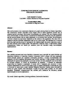
The second example consists of a point-set of 49388 points segmented in 10 primitives. The same parameters as above are used for the size of population, probability of crossover and probability of mutation. Figure 3 illustrates the convergence after 200 generations of a population of size 1000. The solid obtained from the best individual is illustrated by Fig. 4. Evolution of fitness with number of iterations 1000 minimum Value of fitness function
4
800 600 400 200 0 0
50
100
150
200
Number of iterations
Figure 3. Evolution of the fitness of the best individual for a population of size 1000 for the second mechanical part
Evolution of fitness with number of iterations 1000 Value of fitness function
minimum 800 600 400 200 0 0
50
100
150
200
Number of iterations
Figure 1. Evolution of the fitness of the best individual for a population of size 1000 for the first mechanical part
Figure 4. Result for the best individual for the second mechanical part
4.3
Comments
Comparing figures 1 and 3, we find a higher fitness value for the second example. It can be explained by a bigger number of points in the point-set used: the second point-set is approximately 5 times bigger. It can also be explained by a different accuracy in fitting the primitives. The number of points in the point-set has some influence on the algorithm. If this number is too big, it will slow down the evaluation of the fitness function and the overall speed of the algorithm.
5
Conclusion
We have presented a new algorithm based on a simple genetic algorithm to recover an FRep defined by a constructive tree from a segmented point-set and a list of fitted primitives. The algorithm is general, simple and can be easily extended to other operations than the set-theoretic ones: blending operation is an example. This algorithm exhibits similarities with genetic programming. The main difference is that genetic programming uses an infinite length representation for the solutions, where our problem has known finite length solutions. Still it may be interesting to investigate the behaviour of genetic programming and the found solutions on such problem.
Acknowledgements
[6] P. Benko and T. Varady, Direct segmentation of smooth, multiple point regions, Proc. of Geometric Modeling and Processing, Tokyo, Japan, 2002, 169– 178. [7] V. Shapiro and D. L. Vossler, Construction and optimization of csg representations, Computer-Aided Design, 23(1), 1991, 4–20. [8] V. Shapiro and D. L. Vossler, Efficient csg representation of two-dimensional solids, Transaction of ASME, Journal of Mechanical Design, 113, 1991, 292–305. [9] V. Shapiro and D. L. Vossler, Separation for boundary to csg conversion, ACM Transaction on Graphics, 12(1), 1993, 35–55. [10] S. Buchele and R. Crawford, Three-dimensional halfspace constructive solid geometry tree construction from implicit boundary representations, Computer Aided Design, 36(11), 2004, 1063–1073. [11] V. L. Rvachev, L. V. Kurpa, N. G. Sklepus, and L. A. Uchishvili, Method of r-functions in problems on bending and vibrations of plates of complex shape, Technical report, Naukova Dumka, 1973 (in Russian). [12] D. P. Peterson, Boundary to constructive solid geometry mappings: a focus on 3d issues, Computer-Aided Design, 18(1),1986, 3–14.
P.-A. Fayolle acknowledges support by Monbukagakusho, the Japanese Ministry of Education, Culture, Sports, Science and Technology. C. Toinard and C. Rosenberger would like to thank financial support provided by the Conseil G´en´eral du Cher.
[13] V. Shapiro, A convex deficiency tree algorithm for curved polygons, International Journal of Computational Geometry and Applications, 11(2), 2001, 215– 238.
References
[14] A. Pasko and V. Savchenko, Blending operations for the functionally based constructive geometry, Proc. of CSG 94 Set-theoretic Solid Modeling: Techniques and Applications, Winchester, UK, 1994, 151–161.
[1] A. A. G. Requicha and H. B. Voelcker, Constructive solid geometry, Technical Report 25, Production Automation Project, University of Rochester, November 1977. [2] V. L. Rvachev, Geometric applications of logic algebra, Technical report, Naukova Dumka, 1967, (in Russian). [3] V. Shapiro, Theory of r-functions and applications: A primer, Technical Report TR91-1219, Computer Science Department, Cornell University, Ithaca, NY, 1991. [4] A. Pasko, V. Adzhiev, A. Sourin, and V. Savchenko, Function representation in geometric modeling: Concepts, implementation and applications, The Visual Computer, 11(8), 1995, 429–446. [5] T. Varady, R. R. Martin, and J. Cox, Reverse engineering of geometric models – an introduction, Computer Aided Design, 29(4), 1997, 255–268.
[15] V. Savchenko and A. Pasko, Transformation of functionally defined shapes by extended space mappings, The Visual Computer, 14(5), 1998, 257–270. [16] H. Hoppe, Surface reconstruction from unorganized points (PhD thesis, Seattle, WA, USA, 1995). [17] D. Goldberg, Genetic Algorithms in search, optimization and machine learning (Addison-Wesley, 1989).