Sanjeev Pragada and Jayanthi Sivaswamy. Center for Visual Information Technology. International Institute of Information Technology - Hyderabad, Hyderabad ...
Design of Image Adaptive Wavelets for Denoising Applications Sanjeev Pragada and Jayanthi Sivaswamy Center for Visual Information Technology International Institute of Information Technology - Hyderabad, Hyderabad 500032, India Email: {pragadask@research., jayanthi@}iiit.ac.in Abstract—The traditional wavelet based denoising techniques use wavelets which are independent of the image under consideration and the level of noise present in the image. As these techniques which are based on thresholding of wavelet coefficients, rely mainly on the energy compaction and the sparseness of the wavelet representation used, the choice of wavelet is an important consideration. In this paper, for the first time we have proposed a method for designing biorthogonal wavelets for denoising applications from the image at hand using a separable kernel. The denoising performance of this image adapted wavelet is compared primarily against the available biorthogonal wavelets in terms of MSE, PSNR and visual quality, using BayesShrink method which is the current state-of-theart technique in the class of pointwise approaches for image denoising. We have achieved a average improvement of 35% in MSE, over the available biorthogonal wavelets for the low input SNR values (0 to 18db); that is where the actual need for adaptation arises. The results show the efficacy of the approach and the need for adaptive wavelet bases in image denoising.
I. I NTRODUCTION Digital images are often degraded by noise in their acquisition and/or transmission phase. The goal of a image denoising algorithm is to recover the clean image from its noisy version by removing noise and retaining as much as possible the image information. The wavelet transform because of its multiresolution and sparse representations, has been shown to be a powerful tool to achieve these goals. The motivation is that small wavelet coefficients are more likely due to noise and the large coefficients due to the image features. The interest in wavelet based denoising evolved from the seminal work on signal denoising via wavelet thresholding or shrinkage of Donoho and Johnstone in the additive white gaussian noise setting [1], [2]. These authors have proposed two thresholding strategies in which each wavelet coefficient is compared against a threshold; if the coefficient is smaller than the threshold, it is set to zero, otherwise it is kept (hard thresholding) or modified (soft thresholding) [3]. Initially, they have given a mechanism for finding a universal threshold value known as VisuShrink and showed it to be near-optimal in the minimax sense [1]. However, for denoising images, Visushrink is found to yield an overly smoothed estimate, as it is derived under the constraint that with high probability the estimate should be at least as smooth as the image. To overcome this problem, the same authors have proposed a new method called SUREShrink which uses a hybrid of the universal threshold and the SURE
threshold, derived from minimizing Stein’s unbiased risk estimate [4], and has been shown to perform well. Later on, there has been a fair amount of research on threshold value selection for image denoising. One of the most popular was proposed by Chang et al., who derived their threshold in a Bayesian framework, assuming a generalized Gaussian distribution for the wavelet coefficients and is called BayesShrink [5]. This method has a better MSE performance than SUREShrink . In the more recent literature, people have considered the intra and interscale dependencies among the wavelet coefficients and have shown to achieve better denoising performance compared to the pointwise approach. In addition, increasing the redundancy of the wavelet transform has substantially improved the denoising performance. In these views the three main techniques are the BiShrink proposed by Sendur et al. [6], ProbShrink proposed by Pizurica et al. [7] and BLSGSM proposed by Portilla et al. [8]. However, inspite of the improved performances with the use of scale dependencies and redundancy of the wavelet transform, we have used the point-wise techniques and non-redundant wavelet transforms for our comparison because of their simplicity and speed. Our work aims at designing a image matched wavelet which can be used in denoising applications. The motivation for this is that, unlike the Fourier methods, wavelet transforms do not have a unique basis and hence it is natural to seek a wavelet that is best in a particular context. We have explored this fact for the image denoising problem. Over the last decade, there has been a fair amount of research on designing matched wavelets for a particular context [9], [10], [11]. But no work has been reported for the image denoising application in particular. The work done so far in the wavelet based denoising has targeted towards finding the best threshold but not towards finding the best wavelet. We, in this paper have concentrated on the latter problem and our results show the need for adaptive wavelets in image denoising. In image denoising application, it is desirable that the wavelet adapts to the image and not to the noise. We present a technique to design wavelet from noisy image which adapts only to the clean image using statistical properties of noise. These properties help in designing a wavelet which can effectively deal with the noise present in the image, by improving the differential information between the image and noise in the wavelet domain. We have compared denoising performance of our designed biorthogonal wavelets with that of existing set
of biorthogonal wavelets using BayesShrink method which is the current state-of-the-art technique in the class of pointwise approaches. This paper is organized as follows. In Section II, we present our basic work of designing bi-orthogonal wavelets for image denoising applications. In Section III, the overall process of image denoising using our matched wavelets is presented. Experimental results on several images and discussions are given in Section IV and finally Section V deals with the conclusions and future work.
II. D ESIGN OF I MAGE M ATCHED WAVELETS In this section we will describe the algorithm for designing matched wavelets for image denoising. The image matched wavelets are designed using the separable kernel. i.e two sets of 1D matched wavelets are designed, one for row ordering of the image, say a0x (arranging all rows side by side) which contains variation in the horizontal direction only and the other for column ordering of the image, say a0y (arranging all columns one below the other and then taking its transpose) which contains variation in the vertical direction only. Now the design technique for finding 1D matched wavelets for denoising is presented. We use this technique two times, once with a0x as input and obtain the four corresponding filters (h0x , h1x , f0x , f1x ) and next with a0y as input and obtain the four corresponding filters (h0y , h1y , f0y , f1y ). Our criterion for matching is based on maximizing the projection of clean image characteristics in to the scaling subspace rather than the wavelet subspace, using the noise characteristics. Using this matching criteria, we can guarantee that the noise in the coarsest approximation subspace will be less. And, as the thresholding techniques usually leave the coarsest approximation without thresholding, it means that our matching criteria is decreasing the amount of residual noise in the denoising process. A similar approach was proposed by Gupta et al. [11] and their designed wavelets have shown to be having profound application in signal and image compression. However, their wavelets would not work for the denoising applications as they are matched directly to the input image which is the noisy image in denoising applications i.e their technique would maximize the projection of noisy image features into the scaling subspace and not the clean image eplacementsfeatures. Now we present various stages of our algorithm. A. Design of 1D Matched Biorthogonal Bases for image denoising a0 (k)
h0 (−k)
2
a−1 (k)
2
f0 (k)
a ˆ0 (k)
wavelets using a0x and a0y and then by using separable kernel we obtain the image matched wavelets which are suitable for denoising. We first design the analysis highpass filters in each case and use the bi-orthogonal relations to design the remaining filters. Here, we shall talk in terms of 1D signals as we are designing 1D matched wavelets. Design of Analysis High Pass Filter: Using the estimated noise variance, we shall design this filter such that our matching criterion is satisfied. Consider the scenario, where the signal is corrupted with white gaussian noise and we want to remove noise using signal adapted wavelet technique. Let x(t) be the pure signal and n(t) be WGN with independent and identical distribution (i.i.d) with zero mean and σ 2 variance. The noisy signal a(t) is given by, a(t) = x(t) + n(t)
(1)
The sampled value of the signal a(t) is applied as a input to the 2-channel filter bank structure shown in Fig.1 a0 (k) = x(k) + n(k)
(2)
Let a ˆ(t) be the signal reconstructed using only the detail coefficients d−1 (k) and N be the length of the filters in Fig 1. Now the analysis filter which maximizes the error energy between a(t) and a ˆ(t) is obtained using the following equation which is given by Gupta et al. [11]. N −1 X
h1 (p)
p=0
L/2−1 � X k=0
� a0 (2k + p)a0 (2k + r) = 0
(3)
For r=0,1,. . . ,j-1,j+1,. . . ,N-1. where j is the index of middle coefficient of h1 (k). The wavelet designed using the above equation is matched to both signal and noise, where as our goal is to design the filter which is matched only to the signal. To achieve our goal the equation (3) is modified as below N −1 X p=0
h1 (p)
L/2−1 � X k=0
� x(2k + p)x(2k + r) = 0
(4)
For r=0,1,. . . ,j-1,j+1,. . . ,N-1. where j is the index of middle coefficient of h1 (k). Solving the above equation for h1 directly, will need the knowledge of pure signal which we don’t know. So we need to modify equation (4) further so that it can be solved directly. Now, consider the bracketed term in the equation (3) f (p, r) =
L/2−1 2 X a0 (2k + p)a0 (2k + r) L
(5)
k=0
h1 (−k) Fig. 1.
2
d−1 (k)
2
f1 (k)
For p=0,1,. . . ,N-1 and r=0,1,. . . ,N-1 Using equation (2) we can write,
Two channel 1D maximally decimated PR filter bank
Fig.1 shows a 1D two-channel maximally decimated filter bank. We use this filter bank for designing 1D matched
f (p, r) =
L/2−1 2 X [x(2k+p)+n(2k+p)][x(2k+r)+n(2k+r)] L k=0 (6)
=
L/2−1 L/2−1 2 X 2 X x(2k + p)x(2k + r) + x(2k + p)n(2k + r) L L k=0
+
k=0
L/2−1 L/2−1 2 X 2 X n(2k + p)x(2k + r) + n(2k + p)n(2k + r) L L k=0
k=0
Since we assumed that noise is i.i.d and uncorrelated to signal we have, L/2−1 2 X [x(2k + p)n(2k + r)] = 0 L
(7)
k=0
L/2−1 2 X [n(2k + p)x(2k + r)] = 0 L
Design of Remaining Filters in the Matched Biorthogonal Filter Bank: Now the remaining three filters in Fig.1 are obtained using h1 (n) and the biorthogonal relations. That is, Compute f0 (n) using f0 (n) = (−1)n+1 h1 (M − n)
(15)
where M is any odd delay. Now h0 (n) can be calculated using the following two perfect reconstruction conditions and the vanishing moments imposed on f1 (n) N −1 X
h0 (n)f0 (n − 2m) = δ(m)
∀m ∈ Z
(16)
n=0
(8)
N −1 X
k=0
h0 (n)h1 (n) = 0
(17)
n=0
Putting these values in the equation (6), we have
Now let’s say we have imposed p vanishing moments on f1 (n) then, 2 X 2 X f (p, r) = x(2k+p)x(2k+r)+ n(2k+p)n(2k+r) N −1 X L L k=0 k=0 m1 (k) = nk f1 (n) = 0 f ork = 0, 1, . . . , p (18) (9) n=0 Now as auto-correlation function of white Gaussian noise which is transfered to h0 (n) as is zero for any non-zero lag, L/2−1
L/2−1
L/2−1 L/2−1 2 X 2 2 X n(2k+p)n(2k+r) = n (2k+r) L L k=0
; if p = r
k=0
=0
; otherwise
(10)
Let L/2−1 2 X 2 n (2k + r) Γ= L
(11)
k=0
Substituting equation (10) and equation (11) in equation (9), we have L/2−1 2 X f (p, r) = x(2k + p)x(2k + r) + Γ · δ[p − r] (12) L k=0
Thus L/2−1 2 X x(2k + p)x(2k + r) = f (p, r) − Γ · δ[p − r] (13) L k=0
Substituting above equation and equation (5) in to equation (4), we have N −1 X p=0
h1 (p)
�
L/2−1 � X k=0
� � a0 (2k + p)a0 (2k + r) − Γ · δ[p − r] = 0
(14) For r=0,1,. . . ,j-1,j+1,. . . ,N-1. where j is the index of middle coefficient of h1 (k). where Γ is given by equation (11) and can be calculated by assuming a white Gaussian noise with zero mean and known variance.
N −1 X
(−n)k h0 (n) = 0
f ork = 0, 1, . . . , p
(19)
n=0
Equations (16), (17) and (19) can be solved simultaneously to get h0 (n) of p vanishing moments. Now, f1 (n) can be easily found out from equation f1 (n) = (−1)n h0 (M − n)
(20)
Thus, all the four filters of the matched biorthogonal filter bank are derived as explained above. III. E XPERIMENTAL R ESULTS AND D ISCUSSION Now we use the standard wavelet based image denoising algorithm to compare the performance of our matched wavelets with that of fixed biorthogonal wavelets. It includes calculation of forward wavelet transform for the input noisy image and later thresholding of these coefficients with a properly designed threshold and then calculation of reverse wavelet transform of the thresholded coefficents to get the denoised image. The forward and reverse wavelet transforms can be calculated using the eight one dimensional filters (h0x , h1x , f0x , f1x ) and (h0y , h1y , f0y , f1y ) which can be designed using the method described in previous section and the non-redundant separable wavelet system shown in Fig 2. The thresholding strategy used for our comparison is the BayesShrink proposed by Chang et al [5]. The denoising performance of our matched wavelet is compared against existing biorthogonal wavelets for a representative set of standard 8-bit grayscale images such as lena, barbara, baboon, and goldhill, for various noise-levels. In our simulations, we have used 4 level wavelet decomposition obtained by decomposing the LL subband of Fig 2 further and
PSfrag replacements
¯ 0y h ¯ 0x h
2↓
a0 (n1, n2)
¯ 1x h
¯ 1y h
2↓
¯ 0y h
2↓
2↓ ¯ 1y h
Fig. 2.
2↓
2↓
LL
LH
HL
HH
2↑
f0y 2↑
2↑
f1y
2↑
f0y
a ˆ0 (n1, n2)
2↑ 2↑
f0x
f1x
f1y
First level decomposition and reconstruction using separable kernel and matched filters; The bars on filters denote time reversal
Fig. 3.
From left to right: Original Lena , Noisy Lena (sigma = 30) , Denoised using bior3.5, Denoised using matched wavelets
the coarsest approximation coefficients are left unthresholded. Although the thresholding technique, we have used in our simulations [5] was originally designed for orthonormal wavelets, selection of such a threshold is justified as our main motive is to compare the performances of matched wavelets versus fixed biorthogonal wavelets. The results of visual comparison for the lena image are shown in Fig 3 , MSE comparisons for the lena image are shown in Figs 4 and 5, and PSNR comparisons for the representative set are tabulated in Table I. As we can see from Figs 4 and 5, proposed technique performs on an average 35% percent better denoising as compared to non-adaptive biorthogonal wavelets at lower SNR (0-18db) and at higher SNR (>18db), percentage improvement in MSE with respect to non-adaptive wavelet transform decreases. This is a very good improvement in the low SNR cases and that is where the idea of matching is very much required. This is also evident from PSNR comparisons in Table I. At higher SNR, the energy of the noise is very less compared to that of signal. So the wavelet coefficients due to noise are very small and are spread out along all scales as the noise assumed is random, where as coefficients due to signal are very high and most of them exist only for few scales. In this way it is very easy to distinguish signal and noise in wavelet space
by using thresholding technique. Thus, the use of matched biorthogonal wavelets did not yield superior performance to non-adaptive biorthogonal wavelets in this range. However, at lower SNR, the energy of the noise is comparable to the signal. Here, if the correlation between the used wavelet and the image is more, the wavelet representation of the image will be more compact and the distinguishing information between the wavelet coefficients of the signal and noise will be more strong which will help to remove noise in the wavelet space. Thus in this range our adaptive biorthogonal wavelets are performing better than the non-adaptive ones. IV. C ONCLUSION In this paper, we have exploited the fact that wavelet bases are not unique, in designing the best biorthogonal bases for image denoising. We have designed image adaptive biorthogonal wavelet bases from the constraint that most of the energy of clean image should go in to scaling subspace rather than the wavelet subspace. The results showed that adapted biorthogonal wavelets performed much better denoising than the available biorthogonal wavelets for the low input SNR values. However the performance improvement decreased for the high SNR values as explained above. We suggest this approach when noise energy dominates signal energy (low
TABLE I PSNR COMPARISON OF MATCHED WAVELET AND FIXED BIORTHOGONAL WAVELETS σ input PSNR Wavelet Bior3.5 Bior2.2 Bior2.6 Matched Wavelet Bior3.5 Bior2.2 Bior2.6 Matched
5 34.14
10 28.13
15 24.60
35.77 36.22 36.26 31.15
30.61 31.65 31.75 29.69
27.31 28.81 28.87 28.25
32.66 32.57 32.83 27.43
28.36 28.47 28.62 26.01
25.82 26.18 26.25 25.68
20 25 22.10 20.16 Lena 512 X 512 24.92 23.03 26.52 24.92 26.69 25.07 26.74 25.57 Baboon 512 X 512 23.87 22.22 24.46 23.05 24.55 23.10 24.72 24.21
30 18.57
50 14.16
100 8.12
5 34.14
10 28.13
15 24.60
21.47 23.36 23.54 24.57
17.10 19.32 19.31 21.73
11.09 13.34 13.63 16.80
35.22 35.38 35.46 30.75
30.27 31.02 31.08 28.46
27.09 28.27 28.42 27.05
20.87 21.85 21.92 22.83
16.77 18.39 18.47 20.99
11.01 13.12 13.10 15.15
34.81 35.19 35.28 30.34
29.47 29.93 30.01 27.62
26.53 27.20 27.33 26.02
Comparison with bior 2.2,2.4,2.6,2.8 wavelets
60
60
bior 2.6 bior 2.8
% Improvement in MSE
% Improvement in MSE
50 14.16
100 8.12
21.35 23.19 23.34 24.13
17.03 19.15 19.24 21.54
11.13 13.38 13.57 16.68
21.14 22.46 22.53 23.5
16.92 18.72 18.84 20.02
11.02 13.09 13.28 16.15
70
bior 2.4
40
30 18.57
Comparison with Bior : 3.1, 3.3, 3.5, 3.7, 3.9 wavelets
80
bior 2.2
20 25 22.10 20.16 Goldhill 512 X 512 24.74 22.94 26.28 24.61 26.31 24.71 26.67 25.01 Barbara 512 X 512 24.36 22.59 25.30 23.80 25.43 23.95 25.81 24.2
20
0
−20
bior 3.1
50
bior 3.3 bior 3.5
40
bior 3.7 bior 3.9
30 20 10 0
−40
−10 −60
0
5
10
SNR + 1
15
20
25
−20
0
5
10
SNR + 1
15
20
25
Fig. 4. Showing % improvement in MSE over bior2.* series wavelets for Lena image
Fig. 5. Showing % improvement in MSE over bior3.* series wavelets for Lena image
SNR), because that is where the actual need for adaptation arises. Although our focus in this paper is on the adaptive biorthogonal wavelets, the adaptation can also be tried for orthonormal wavelets for yielding better denoising performance than the existing orthonormal wavelets.
[8] J. Portilla, V. Strela, M. Wainwright, and E. Simoncelli, “Image denoising using scale mixtures of gaussians in the wavelet domain,” IEEE Transactions on Image Processing, vol. 12, no. 11, pp. 1338–1351, 2003. [9] A. H. Twefik, D. Sinha, and P. Jorgensen, “On the optimal choice of a wavelet for signal representation,” IEEE Transactions on Information Theory, vol. 38, no. 2, pp. 747–765, 1992. [10] J. O. Chapa and R. M. Rao, “Algorithms for designing wavelets to match a specified signal,” IEEE Transactions on Signal Processing, vol. 48, no. 12, pp. 3395–3406, 2000. [11] A. Gupta, S. D. Joshi, and S. Prasad, “A new approach for estimation of statistically matched wavelet,” IEEE Transactions on Signal Processing, vol. 53, no. 5, pp. 1778–1793, 2005.
R EFERENCES [1] D. L. Donoho and I. M. Johnstone, “Ideal spatial adaptation by wavelet shrinkage,” Biometrika, vol. 81, no. 3, pp. 425–455, 1994. [2] ——, “Adapting to unknown smoothness via wavelet shrinkage,” Journal of the American Statistical Association, vol. 90, no. 432, pp. 1200–1224, july 1995. [3] D. L. Donoho, “De-noising by soft-thresholding,” IEEE Transactions on Information Theory, vol. 41, no. 3, pp. 613–627, 1995. [4] C. M. Stein, “Estimation of the mean of a multivariate normal distribution,” The Annals of Statistics, vol. 9, no. 6, pp. 1135–1151, 1981. [5] G. Chang, B. Yu, and M. Vetterli, “Adaptive wavelet thresholding for image denoising and compression,” IEEE Transactions on Image Processing, vol. 9, no. 9, pp. 1532–1546, 2000. [6] L. Sendur and I. W. Selesnick, “Bivariate shrinkage functions for wavelet-based denoising exploiting interscale dependency,” IEEE Transactions on Signal Processing, vol. 50, no. 11, pp. 2744–2756, 2002. [7] A. Pizurica and W. Philips, “Estimating the probability of the presence of a signal of interest in multiresolution single- and multiband image denoising,” IEEE Transactions on Image Processing, vol. 15, no. 3, pp. 654–665, 2006.