Development and application of a coupled-process parameter ...

PII: S 0 3 0 9 - 1 7 0 8 ( 9 8 ) 0 0 0 4 9 - 9

Advances in Water Resources Vol. 22, No. 8, pp 841±853, 1999 Ó 1999 Elsevier Science Ltd Printed in Great Britain. All rights reserved 0309-1708/99/$ ± see front matter

Development and application of a coupled-process parameter inversion model based on the maximum likelihood estimation method Alex S. Mayer* & Changlin Huang Department of Geological Engineering and Sciences, 1400 Townsend Drive, Michigan Technological University, Houghton, MI 49931, USA (Received 22 June 1998; accepted 14 November 1998) The coupled ¯ow-mass transport inverse problem is formulated using the maximum likelihood estimation concept. An evolutionary computational algorithm, the genetic algorithm, is applied to search for a global or near-global solution. The resulting inverse model allows for ¯ow and transport parameter estimation, based on inversion of spatial and temporal distributions of head and concentration measurements. Numerical experiments using a subset of the three-dimensional tracer tests conducted at the Columbus, Mississippi site are presented to test the model's ability to identify a wide range of parameters and parametrization schemes. The results indicate that the model can be applied to identify zoned parameters of hydraulic conductivity, geostatistical parameters of the hydraulic conductivity ®eld, angle of hydraulic conductivity anisotropy, solute hydrodynamic dispersivity, and sorption parameters. The identi®cation criterion, or objective function residual, is shown to decrease signi®cantly as the complexity of the hydraulic conductivity parametrization is increased. Predictive modeling using the estimated parameters indicated that the geostatistical hydraulic conductivity distribution scheme produced good agreement between simulated and observed heads and concentrations. The genetic algorithm, while providing apparently robust solutions, is found to be considerably less ecient computationally than a quasi-Newton algorithm. Ó 1999 Elsevier Science Ltd. All rights reserved Key words: Parameter inversion, Maximum likelihood estimation, Groundwater ¯ow, Transport.

o…/C† ; ot subject to initial conditions on R

1 INTRODUCTION 1.1 Coupled-process parameter inversion During the past few decades, computational models of groundwater ¯ow and solute transport have been developed to predict solute concentrations for contaminated subsurface systems. The commonly used models are based on the following partial di€erential equations on R r…Krh† ‡ W ˆ Ss

*

oh ; ot

r…Dr/C† ÿ r…Cq†M ˆ Ss

…2†

h ˆ h0 and C ˆ C0 at t ˆ t0

…3†

generalized hydraulic head boundary conditions on Ch bh rh
n ˆ nh …Hb ÿ h† ‡ ch …4† and generalized solute concentration boundary concentrations on CC bC rC
n ˆ nC …Cb ÿ C† ‡ cC ;

…1†

…5†

where K is the hydraulic conductivity tensor, h the hydraulic head, W the ¯uid sink or source, Ss the speci®c storage, D the hydrodynamic dispersion tensor with components Dij ˆ D0 ‡ …aL ÿ aT †vi
vj =jvj ‡ aT jvjdij , D0

Corresponding author. 841

842

A. S. Mayer, C. Huang

the molecular di€usion coecient; aL and aT are the longitudinal and transverse dispersivities, respectively, vi the pore velocities along Cartesian coordinate axes i; dij the Kronecker delta function, / the porosity, C is the solute concentration, q is the Darcy velocity, q ˆ ÿKrh, M is a solute sink or source term, b, n, and c are values of boundary conditions as de®ned in Table 1, n is the unit vector normal to the domain boundary …Ch or CC †; Hb and ch are the prescribed boundary head and ¯ow ¯ux, respectively, and Cb and cC are the prescribed boundary solute concentration and mass ¯ux, respectively. The success of concentration predictions requires accurate characterization of parameters such as hydraulic conductivity distributions and dispersion coecients over the problem domain and its boundaries. In practice, eqns (1)±(5) are solved by numerical methods. When numerical models are used to predict solute concentrations in the aquifer, the parameters must be identi®ed in discrete intervals over the entire domain. Unfortunately, the parameters generally are not measurable at the scale of discretization, since the few available parameters from the ®eld usually are taken from a limited region and are insucient to fully characterize parameter variations over the aquifer domain. The choice of appropriate parameters and their spatial distributions remains the most serious problem for producing accurate predictions of solute transport and for development of cost-e€ective remediation designs for contaminated sites. Inversion of head and concentration measurements can be useful for estimating model parameters. However, head and concentration measurements are limited to a ®nite number of observation points and frequently are corrupted by noise. The limited number of head and concentration measurements and the errors in these measurements produces an ill-posed inverse problem. The ill-posedness of the inverse problem is characterized by non-uniqueness and the instability of numerical solutions to the inversion problem. The inverse problem usually is formulated as the minimization of an objective function, implying that a global minimum associated with the best parameter estimates can be found. The presence of multiple local minima can result in nonunique solutions even if the parameters are identi®able or sensitive to model output. This non-uniqueness, called discrete non-uniqueness, cannot be prevented in general1.

Table 1. Boundary conditions Boundary type

bu

nu

cu

Dirichlet boundary Neuman boundary Mixed boundary

0 b b

1 0 n

0 c c

1.2 Previous work on parameter inversion Extensive investigations have been made to estimate ¯ow parameters in eqn (1) from hydraulic head measurements. The evolution of concepts in ¯ow inversion is brie¯y described by Carrera and Neuman2. A review and summary of the inverse problem solution through ¯ow modeling is given by Yeh3 and Carrera1. McLaughlin and Townley4 reviewed recent advances in ¯ow inverse problems and provided a more general formulation and methodology for parameter estimation. Solution of the inverse problem for mass transport processes has not been studied as extensively as the ¯ow inverse problem. Inversion of mass transport processes usually includes assumptions that the ¯ow ®eld is known exactly and that one- or two-dimensional transport with equilibrium chemistry is an acceptable idealization for mass transport processes (e.g. Refs.5,6). A brief review of mass transport process inversion can be found in Ref.1. Stochastic approaches for ¯ow and transport inversion are reviewed by Kitanidis7. Even less research has been conducted on the coupled ¯ow-mass transport inverse problem, but it is receiving more attention (Ref.8). The lack of published work on transport process inversion or coupled ¯ow-mass transport inversion is a consequence of uncertainty in hydraulic parameters and the computational diculties that arise in solving the solute transport equations. Uncertainty in the hydraulic conductivity ®eld will produce an uncertain ¯ow ®eld, which can further result in meaningless estimates of solute transport parameters. Numerical problems with the transport solution, such as instability, oscillations, and numerical dispersion, can arise for certain combinations of model parameters (Ref.1). Strecker and Chu9 presented a ¯ow-mass transport inversion procedure to estimate ¯ow and solute transport parameters in a sequential programming formulation. In their work, errors from the ®rst step of estimating hydraulic conductivity based on head measurements were incorporated into the second step where dispersivities were estimated from solute concentration measurements. Since the ¯ow inversion problem is loosely coupled with the transport inversion problem, the sequential approach can result in extreme values of dispersivities. Mishra and Parker10 compared sequential parameter estimation procedures with a simultaneous (coupled-process) parameter estimation procedure for a one-dimensional, transient, unsaturated ¯ow tracer problem. They concluded that the coupled-process procedure resulted in smaller estimation errors of dispersivity, dispersivity scale factors, saturation index exponent, and hydraulic conductivity. Wagner and Gorelick11 developed a methodology to incorporate ¯ow and transport process modeling with nonlinear, least squares, multiple regression for the simultaneous match of both head and concentration

Development and application of a coupled-process parameter inversion model measurements. Application of this approach to the Gloucester Land®ll site indicated that coupled-process parameter estimation, where both head and concentration data are matched, reduced the prediction uncertainty by about 50%, when compared to parameter estimates from matching concentration data alone39. Sun and Yeh8 demonstrated that hydraulic conductivity was identi®able through model inversion of concentration observations, by use of the adjoint state sensitivity method. Coupled-process inversion problems, including ¯ow-¯ow, ¯ow-heat, and ¯ow-mass transport coupling, were reduced to a vector form by formulating the inversion problems as multi-objective optimization problems. Sun and Yeh8 describe a procedure for deriving adjoint state equations to obtain gradient vectors of the objective functions and the sensitivity coecients. The procedure was applied to a two-dimensional, coupled ¯ow-mass transport problem. Woodbury and Smith12 and Woodbury et al.13 made a comprehensive study of the theory and application of coupled ¯ow-heat transport inversion, which is a similar problem to coupled ¯ow-solute transport inversion. In the example problem discussed in Woodbury et al.13, hydraulic conductivity and various boundary values were estimated from temperature and head measurements. Hyndman et al.14 presented a split inversion method combined with Wagner and Gorelick's nonlinear regression techniques11 to estimate e€ective zonation parameters of hydraulic conductivity and dispersivity. The parameters were inverted from seismic and tracer test data with pre-selected spatial covariance structural parameters. Harvey and Gorelick15 developed a coupled parameter estimation method for mapping ¯ow parameters from solute arrival time, hydraulic heads, and local measurements of hydraulic conductivity. Barlebo et al.16 used a nonlinear regression approach to simultaneously invert ¯ow and transport parameters using head and concentration data from the MADE tracer experiments. 1.3 Scope of the present contribution Coupled process inversion has been shown to produce improved estimates of ¯ow and transport parameters when compared to single process inversion. Many different approaches have been adopted for the formulation and numerical solution of the coupled inverse problem. However, generalized approaches to solving the statistical and numerical diculties associated with coupled process inversion have not been developed. Furthermore, there have been very few attempts to evaluate the performance of transport or coupled ¯ow and transport inversion models against ®eld data. An integrated approach for the estimation of ¯ow and transport parameters by matching head and concentration measurements simultaneously is developed in this work. Maximum likelihood estimation is applied

843

to formulate the identi®cation criterion. A simulation± evolution algorithm, the genetic algorithm, is used to solve the maximum likelihood formulation. The integrated approach is applied to a three-dimensional subset of the MADE2 tracer test data set17,18. Hydraulic conductivity distributions are estimated as either e€ective, zoned values or via geostatistical parameters. E€ective dispersivities and retardation coecients also are estimated. Initial soft and hard information for the site is incorporated to determine the constraint sets of the parameters to be estimated. The estimated parameters are applied in a predictive mode to further evaluate the inversion approach and the parametrization schemes. The performance of the genetic algorithm is compared to a more conventional optimization algorithm. 2 COUPLED PROCESS INVERSE MODEL 2.1 Formulation of the coupled inverse problem The basic idea of the indirect inverse problem is to minimize the model output error criterion and to iteratively improve parameter estimates until the model output is suciently close to the measurements. In this work, the maximum likelihood estimation (MLE) formulation of the ¯ow inversion problem of Carrera and Neuman2,19 is extended to the coupled ¯ow-mass transport inversion problem. MLE is applied to estimate the ``most likely'' parameters for a speci®c model structure, i.e. the governing ¯ow or mass transport equations, parametrization scheme, and the structure of measurement errors. MLE views parameters as ®xed, but unknown and uncertain variables. In Refs.2,19, it is assumed that all measurements are transformed to yield multivariate normal distributions of the prior errors. Following the same assumption and formulation of equations, the likelihood function of prior measurement errors …z ÿ z† for the coupled ¯ow-mass transport problem can be written as   1 ÿN =2 T exp ÿ …z ÿ z† Qÿ1 …z ÿ z† ; L…b=z † ˆ …2pjQj† 2 …6† 

T

T

where z ˆ …h ; C ; p † and z ˆ …h; C; p† are the measurement vectors and true value vectors, respectively, for T the state variables (h, C) and parameters (p), b ˆ …p; h† is the vector of all unknown parameters, p, and unknown statistical parameters, h ˆ …r2h ; r2C ; r2j ; q; . . .†T , used to de®ne prior error distributions, r2h , r2C , and r2j are positive scalars which can be known or unknown prior variances of solute concentrations, head, and the jth parameter type, and q is the temporal correlation matrix at any location xi . Usually, q is assumed to be constant over the domain, in order to reduce the computational burden.

844

A. S. Mayer, C. Huang

The covariance matrix (Q) of the prior errors is a symmetric positive de®nite matrix. The matrix Q reduces to a block diagonal form with diagonal elements …Qh ; QC ; Qpj †, if it is assumed that the prior measurement errors for the state variables and parameters are mutually independent. The prior measurement errors are independent if the state variables and parameters are obtained with independent measurement instruments, which is usually the case. Only the posterior estimation errors are correlated with each other because both the state variables and parameters are produced from the same groundwater simulator. In order to further reduce the computational burden of solving the inverse problem, we assume the prior estimates of the various parameter types are mutually uncorrelated. Thus, Qp is a block diagonal matrix with a diagonal component Qpj . In Q, Qh ˆ r2h Vh , QC ˆ r2C VC , and Qpj ˆ r2j Vj are the covariance matrices of the prior errors for the state variables and parameters. Vj is a known, symmetric positive de®nite matrix2. The symmetric positive de®nite matrix Vu can be expressed as Vuijkl ˆ Xuij
qukl ;

…7†

where the subscript u ˆ h or C, Vuijkl is the covariance between prior errors of the state variables at location xi and time tk , Xuij is the covariance between prior errors of the state variables at any xi and xj , and qukl is the temporal correlation between prior errors of the state variables between times k and l at any xi . Usually, Xuij is interpolated by kriging or residual kriging if the state variable is non-stationary (Ref.20). The matrix qukl represents systematic errors in the prior errors in the state variables. This matrix can be represented by an autoregressive model if the sampling interval is constant. Other properties of Vu are discussed in Ref.2. The modi®ed identi®cation criterion, based on the MLE formulation of the ¯ow inverse problem found in Ref.2, using a negative log likelihood basis, is J ˆ N ln…2p† ‡

X Ju

‡

X Jj

r2j u j X X ‡ …Nxu ln jqu j ‡ Ntu ln jXu j† ‡ ln jVj j r2u

u

j

X X Nu ln r2u ‡ Nj ln r2j ; ‡ u

…8†

j

where N is the total number of measurements of prior data, X X X X Nu ‡ Nj ˆ Nxu Ntu ‡ Nj : …9† Nˆ u

j

u

j

Ju is the residual criterion for the state variables …u ˆ h; C†, T

 Ju ˆ …u ÿ u† Vÿ1 u …u ÿ u†

…10†

and Jj is the penalty criterion of the jth parameter type pj

T

 Jj ˆ …pj ÿ p† Vÿ1 j …pj ÿ p†

…11†

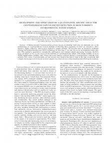
In practice, the prior error variances are applied to normalize the variances r2h , r2C , and r2j so that the discrepancy in units among various kinds of measurements can be reduced (Ref.21). Here, an empirical procedure is adopted from Ref.10 to normalize the variances and eliminate the dimensionality problem with the prior measurements. 2.2 Search method The genetic algorithm (GA) is an evolutionary search algorithm that has been applied to a wide range of optimization problems in science and engineering. Applications of GAs for inversion problems in the earth sciences primarily have been concentrated in geophysics, especially in seismology. Sambridge and Drijkonigen22 and Sambridge and Gallagher23 applied GAs for the inversion of real-time refraction data. Scales et al.24 applied GAs as a global optimization methods for a multi-modal inversion problem. Other seismological applications include that of Jin and Madriaga25 on inversion of the background velocity ®eld and Nolte and Frazer26 on inversion of vertical seismic pro®ling. The philosophy of GAs is analogous to the evolution of biological natural selection processes. GAs search from a population of solutions, rather than a single solution as in traditional, gradient-based optimization methods. Within a given environment and a set of initial populations or solutions, more successful solutions will survive and propagate. There are many variations of GAs, but the basic computational steps of GAs in each complete search cycle are similar and are described in Fig. 1. Each search cycle consists of one or more operations on each candidate solution and the cycle is repeated until a suitable solution criterion is reached. Unlike the traditional gradient-based approaches, there is no simple way to express the methodology in a few mathematical equations. Further discussion and fundamentals are given by Holland27, Goldberg28, and Davis29,30. In summary, it is relatively straightforward to implement a genetic algorithm for a given problem once the principle of the methodology is understood; but usually a preliminary study is conducted to achieve the most ecient combinations of operational parameters. Appropriate operational parameter combinations can produce a near global solution both rapidly and robustly. However, unexpected results can result from unrealistic formulation of the problem, especially with regard to the constraint sets. 2.3 Parametrization schemes Distributions of the ¯ow and transport parameters can be described in several ways, including uniform, e€ective homogeneous parameters; zones of e€ective parameters; or structured distributions based on stochastic models.

Development and application of a coupled-process parameter inversion model

845

p vector, where Y ˆ ln…K†. The stochastic representation also requires the selection of a covariance model to represent the geostatistical structure of the hydraulic conductivity ®eld. Once a covariance model is selected, kriged ®elds of hydraulic conductivity can be generated, based on the measured hydraulic conductivities and on the estimates of the variance and the scale parameters. The covariance model also is incorporated into the MLE formulation. Errors in the measured hydraulic conductivities are allowed, assuming that the measurement errors are independent of one another. The head and concentration measurements are not used directly to estimate the ln(K) ®eld through co-kriging, as was done in Ref.31. Instead, measurements of hydraulic conductivity alone are used to condition the ln(K) ®eld; the head and concentration measurements indirectly in¯uence the estimation of the ln(K) ®eld. 3 APPLICATION TO THE MADE SITE TRACER TEST 3.1 Overview of tracer test and modeling

Fig. 1. Flow chart for the genetic algorithm.

In the case of e€ective parameters, the values of these parameters are estimated by the MLE formulation by simply including them as explicit variables in the p vector. When stochastic models are used to describe parameter distributions, the parameters associated with the stochastic ®eld are estimated with the MLE formulation31. In this work, we consider only the hydraulic conductivity to be a stochastic parameter. This approach di€ers from that of Kitanidis and Vomvoris31, where point estimates of hydraulic conductivity and head are chosen to be stochastic variables. The scale parameters, ki , and variance, r2Y , associated with the hydraulic conductivity ®eld are included in the

The MADE experiment was a large-scale, natural gradient, ®eld tracer study conducted in a substantially heterogeneous, alluvial aquifer near Columbus, Mississippi. A complete description of the ®eld tracer site, experimental methods, and data analysis is given by Boggs et al.17, Adams and Gelhar32, Rehfeldt et al.33, and Boggs and Adams17. The input data for the example application is taken from a subset of the database of the MADE2 tracer test, which was conducted in 199034. The MADE2 tracer test consisted of a pulse injection of a conservative tracer solution (tritiated water) into the saturated zone of the aquifer. Spatial distributions of tracer concentrations were monitored at one- to threemonth intervals using an array of over 300 multilevel samplers spaced about 10 m apart in the horizontal direction and 0.38 m apart in the vertical direction. Hydraulic conductivity measurements were obtained from borehole ¯owmeter tests at 11 fully penetrating piezometers in the near-®eld region of the experimental site. These and other hydraulic conductivity measurements in the previous MADE1 test are used for generating the hydraulic conductivity ®elds in this work. The MADE2 test was selected as an application of the coupled inverse model because (1) the data is generally accepted to be of reasonably high quality, (2) previous work on the site has established ``true'' or ``likely'' values, or at least reasonable ranges, of the parameters to be estimated and (3) the site is representative of a moderate level of aquifer heterogeneity and thus represents a rigorous test of the parameter inversion model. The purpose of this application is to test the parameter inversion model, not to validate or prove any previous estimates of ¯ow and transport parameters at

846

A. S. Mayer, C. Huang

the Columbus site. It should be noted that some problems with the MADE data sets have been identi®ed, such as surpluses and de®cits in the global, measured tritium mass after the MADE2 tracer injection and questionable hydraulic conductivity measurements from the MADE1 test16. In order to reduce the computational burden of solving the coupled inverse problem, a subset of the MADE2 database is used. The physical dimensions of the aquifer subset are 23 m wide by 90 m long by 5 m deep. The aquifer subset is discretized into 23 by 90 by 5layer ®nite-di€erence grid, resulting in grid block sizes of 1 m by 1 m by 1 m. The groundwater ¯ow and solute transport simulators used in this work are MODFLOW35 and MT3D36, respectively. Two separate, temporal data sets from the MADE2 tracer test are used in this work: (1) a data set taken from the ®rst 132 days of the test was used for inversion modeling and (2) a data taken set taken from the next 92 days was used for predictive modeling. The boundary conditions used in the simulations include constant heads along the peripheral boundary and zero ¯ux at the bottom of the aquifer. The constant head boundary values along the peripheral ®nite di€erence cells were interpolated from the full-scale hydraulic head data set. These assumed boundary conditions are arti®cial due to the fact that the heads along the boundary could have varied over the period when the tracer data was obtained. In addition, the existence of a zero vertical ¯ux component has not been veri®ed. 3.2 Inversion modeling The initial conditions and data sets of hydraulic heads and tritium concentrations used for the parameter inversion are drawn from observations taken between days 27 and 132 after the tracer injection, including four head measurement data sets (days 27, 48, 111, and 132), and two concentration data sets (days 27 and 132). During this interval, precipitation and recharge were relatively small and hydraulic head ¯uctuations were minor. Fig. 2 shows the hydraulic heads measured at the end of the inversion modeling interval (day 132). The head distribution indicates that a non-uniform ¯ow condition exists in the aquifer subset. The trend in head distributions is consistent with the results of Adams and Gelhar32 and suggests that the aquifer subset may be representative of the full-scale aquifer. The values along the constant head boundary are interpolated from the day 27 head measurement data set. The initial tritium concentrations are taken from the appropriate subset of the MADE2 data set. Fig. 3 shows the measured tritium concentrations at the end of inversion interval in layer 4, which, along with layer 5, is where the majority of the tracer is found. The input parameters for the MLE and GA formulations and simulation models are listed in Table 2. Two parameters, porosity and bulk density, are

Fig. 2. Measured hydraulic heads at day 132 (end of inversion modeling interval).

Fig. 3. Measured tritium concentrations in layer 4 at day 132 (end of inversion modeling interval). Table 2. Parameters employed in MLE/GA applications MLE parameters r2u ˆ 1 r2j ˆ 1 Ntu ˆ 0 Nj ˆ 0 jVj j ˆ 1 jqu j ˆ 1 jXu j ˆ 1 GA parameters Probability of crossover: 0.6 Probability of mutation: 0.0033 Population size: 30±40

treated as known and uniform: / ˆ 0:33 and qb ˆ 1:77 g/cm3 , where qb is the aquifer material bulk density. 3.3 Parametrization schemes The coupled process inversion model was applied to several di€erent parametrization schemes, with each scheme providing successively more information. The allowable ranges for each parameter considered in these schemes are given in Table 3. In Scheme A, the aquifer is

Development and application of a coupled-process parameter inversion model Table 3. Range of parameters employed in parametrization schemes Parameter ˆ [minimum, maximum] K ˆ [0.0, 6.0] m/day r2Y ˆ ‰0:6; 3:5Š kx ˆ ky ˆ ‰0:3; 12Š m kz ˆ ‰0:1; 3:0Š m aL ˆ ‰0:12; 9:0Š m aT ˆ ‰0:05; 6:2Š m p1 ˆ p2 ˆ [0, 35] deg

Applicable scheme A, B C, D, E C, D, E C, D, E All All D, E

treated as a homogenous, isotropic aquifer. E€ective parameters for hydraulic conductivity (K), longitudinal dispersivity …aL † and transverse dispersivity …aT † are estimated. Scheme B involves a zonation approach, where three vertically zoned, e€ective hydraulic conductivities, K1 ; K2 , and, K3 , corresponding to the top two layers, middle two layers and bottom layer, respectively, are identi®ed. Each zone is assumed to have a distinct, isotropic value of hydraulic conductivity. E€ective values of aL and aT also are estimated for the aquifer system in Scheme B. Instead of identifying one or more e€ective hydraulic conductivities, Schemes C, D and E involve identi®cation of stochastic parameters (variance and correlation scales) for a ln(K) ®eld. The ln(K) ®elds are generated by kriging, assuming that the ln(K) covariance model is an exponential model, as in 2 !1=2 3 2 2 2 f f f 1 5; ‡ 2‡ 3 …12† C…f† ˆ r2Y exp 4 ÿ k21 k22 k23 where r2Y is the variance of the ln(K) ®eld, ki are the correlation scales in the principal coordinate directions i, and fi is the separation vector in the principal coordinate direction i. Equation (12) describes a three-dimensional, statistically anisotropic covariance function. The principal directions of the correlation scales are assumed to coincide with the x, y and z axes. The ln(K)®elds are kriged from 22 measurements of hydraulic conductivity obtained from the MADE1 and MADE2 databases. Of these 22 measurements, ®ve were arbitrarily chosen for calculating the model errors in the objective function. In Scheme C, the variance and correlation scales associated with an isotropic ln(K) ®eld are estimated, along with e€ective longitudinal and transverse dispersivities. It has been suggested that a high permeability zone crosses the tracer site, since geological interpretations of aerial photographs indicate the potential of an ancient river across the middle region of the site18. Scheme D incorporates this soft information by assuming that an anisotropic condition exists. The angles of anisotropy, p1 and p2 , are estimated, where p1 and p2 , are the angles between the principal directions of hydraulic conductivity and the principal ¯ow directions in the horizontal plane. Anisotropy in the horizontal plane is imposed on

847

the hydraulic conductivity ®eld by introducing o€-diagonal terms in the hydraulic conductivity tensor. The principal direction of hydraulic conductivity and the vertical direction of ¯ow are assumed to be aligned. Scheme D also involves estimation of the variance and correlation scales of the ln(K) ®eld and e€ective longitudinal and transverse dispersivities. Although tritium, the tracer chemical used in the MADE2 tracer tests, is considered to be conservative, it has been noted that the mass recovery of the tracer chemical at the end of the test was relatively low. Tracer sorption has been suggested as a potential explanation of the low mass recovery (Ref.17). Scheme E is identical to Scheme D, except that it considers the potential of tracer sorption by identifying the e€ective, linear aquifer material±water partitioning coecient …Kd †. A retardation factor …Rf ˆ 1 ‡ Kd qb =/† is incorporated into eqn (2) to allow for estimation of Kd . 3.4 Predictive modeling The parameters estimated for each parametrization scheme were used to predict ¯ow and transport from the end of the inversion modeling interval (day 132 after tracer injection) until day 224. A hydraulic head data set from day 196 and a tritium concentration data set from day 224 were used for veri®cation of the simulation results. There are 48 and 302 observations in the head and concentration veri®cation data sets, respectively. Fig. 4 shows the measured hydraulic heads from day 196. Comparison of Fig. 2 and Fig. 4 indicate that groundwater levels have generally increased from day 132 to day 196. The general direction of ¯ow, which is in approximately the y-direction, apparently has remained relatively constant, but the gradient in this direction has increased by about 50%. The head and gradient increases are presumably due to recharge and must be accounted for in the ¯ow model. Instead of explicitly accounting for recharge in the predictive simulations, the head boundary conditions are changed over time,

Fig. 4. Measured hydraulic heads at day 162 (during prediction modeling interval).

848

A. S. Mayer, C. Huang

according to observed heads in the vicinity of the model boundaries. The transient ¯ow modeling in the predictive interval (day 132 to day 196) was conducted over ten time steps. At each time step, the head boundary values were interpolated in time and space from the measured heads and incorporated as the constant boundary heads for the respective time step. An additional head data set from day 162 was used for interpolating the constant head boundary values through day 196. 4 RESULTS AND DISCUSSION 4.1 Parameter inversion results The results from Schemes A and B are found in Table 4, including the most likely estimates of the parameters, the beginning (Ji ) and ®nal (Jf ) values of the total residual criteria, and the number of generations required for convergence. The results in Table 4 show that the three-zoned parametrization (Scheme B) reduces the total residual by about 250 times when compared to

Table 4. Parameter estimates for Schemes A and B Parameter K (m/day) aL (m) aT (m) Ji (residual) Jf (residual) Number of generations required for convergence a b c d

Scheme A 3.1 2.5 0.57 4.37 ´ 106 1.22 ´ 106 10

Scheme B 2.9/2.7/1.3 2.8 0.61 8.05 ´ 104 4.94 ´ 104 11

Reference values a

0.03±5.1 b 1.2±3.1 c 0.3±0.6 c N/A d N/A N/A

K ˆ K1 /K2 /K3 . Boggs et al. 18. Adams and Gelhar 32. N/A: not applicable.

the single, e€ective parametrization (Scheme A), even though the three-layer zonation is purely arbitrary. Table 4 also lists measured or inferred values from the MADE1 and MADE2 studies for the overall hydraulic conductivity and dispersivities32,18. Since these reference values were generated for the full site and thus represent a physical scale approximately three times the scale used in the numerical experiments, comparisons between the reference and estimated values are somewhat suspect. However, it is worth noting that all of the estimated values fall within the range of reference values. The results for Schemes C, D, and E are given in Table 5. When comparing the results from the zoned parametrization (Scheme B) with that of the geostatistical simulation parametrization (Scheme C), it is found that the latter reduces the total residual by about 4.5 times. The values of longitudinal and transverse dispersivities for Scheme C are signi®cantly smaller than those in Schemes A and B. This result may indicate the stochastic hydraulic conductivity distribution in Scheme C is accounting for a portion of the macroscopic dispersion estimated in Schemes A and B. Comparisons of the results for Schemes C and D indicate statistically that there is an anisotropic condition in the hydraulic conductivity ®eld. The identi®cation of the horizontal anisotropic angle (Scheme D) reduces the residual by 8%, compared to the residual in Scheme C where anisotropic angle is not identi®ed. Although the reduction gained from estimating anisotropic angles is small for the aquifer subset considered in the numerical experiments, it may be more signi®cant for the full-scale site. In Scheme E, the model identi®es the linear aquifer material±water partitioning coecient (Kd ). The zero value estimated for the (Kd ) is consistent with the conservative properties of the tritium tracer and thus does not o€er an explanation for the poor mass recovery of the tracer. The reference parameter values shown in the last column of Table 5 for Schemes C±E are deduced from

Table 5. Parameter estimates for Schemes C, D, and E Parameter

Scheme C

Scheme D

Scheme E

Reference values

r2Y kx ˆ ky (m) kz (m) aL (m) aT (m) p1 ˆ p2 (deg.) Kd (cm3 /g) Ji Jf Number of generations required for convergence

1.0 5 0.65 1.8 0.31 N/A N/A 2.41 ´ 107 1.09 ´ 104 13

1.4 5.1 0.66 1.6 0.52 15 N/A 2.21 ´ 104 1.01 ´ 104 20

1.7 5.2 0.67 1.6 0.39 10.1 0.0 2.27 ´ 104 1.02 ´ 104 31

2.3±3.1 a 4.0±6.9 a 0.6±1.1 a 1.2±3.1 b 0.3±0.6 b N/A d 0.0 c N/A N/A N/A

a b c d

Rehfeldt et al. 33. Adams and Gelhar 32. Boggs et al. 18. N/A: not applicable.

Development and application of a coupled-process parameter inversion model ®eld measurements and moment calculations obtained in the Columbus site analyses32,17,18,33. Most of the estimated values fall within the range of the reference values. The exception is the value of the variance of the ln(K) ®eld, where the estimated values for Schemes C±E is lower than the range estimated by Rehfeldt et al.33 Since the reference values were obtained from a larger scale and the ln(K) variance may be scale dependent, it is not surprising that the estimated parameter values are lower than the reference values. The ln(K) variances estimated for Schemes C±E are signi®cantly di€erent, but the ®nal value of the MLE residual criteria for these schemes are similar. In an effort to determine whether the results of the MLE estimates are insensitive to the estimated ln(K) variances, the inversion modeling for Schemes C and E were reexecuted with a ®xed value of ln(K) variance, r2Y ˆ 1:4. This value represents the average of the estimated ln(K) variances for Schemes C±E and happens to correspond the value estimated for Scheme D. It was found that (1) the values of the remaining, estimated parameters were similar to those estimated when r2Y was allowed to vary and (2) the MLE residual criteria also were similar to those found when r2Y was allowed to vary. The MLE estimates appear to be relatively insensitive to the value of the ln(K) variance. However, this result is not surprising, since kriged ln(K) ®elds are independent of the variance.

849

aquifer subset over the predictive interval. The sample standard deviation of the measured heads in the aquifer subset at day 196 is 0.18 m. The average head residuals for Schemes are C, D, and E are quite small relative to the spatial standard deviation of the measured heads, indicating that the ¯ow portion of the predictive modeling is accurate for these schemes. The heads produced by Scheme B also appear to be relatively accurate, whereas Scheme A is signi®cantly less accurate than the other schemes. In Fig. 5, a kriged map of the point residuals between the measured and predicted hydraulic heads at day 162 is shown for Scheme C. The spatial distribution of the residuals in Fig. 5 is typical of the parametrization schemes, where the predicted heads are increasingly over-predicted for higher values of x and y. This bias is likely a result of the arti®cial, constant-head boundary conditions that are imposed on the heads. The di€erences between the predicted concentrations provided by Schemes A, B and C±E are signi®cant. The average, normalized errors for Schemes A and B are equivalent to average errors of 190% and 57%, which would seem to be unacceptably large. On the other hand, the normalized error for Schemes C±E are in the range of a 20% average error. This magnitude of error is reasonably good for a predictive solute transport simulation. Fig. 6(a) shows a kriged map of the point

4.2 Predictive modeling Table 6 shows the results of the ¯ow and transport predictions using each parametrization scheme. The hydraulic head and tritium concentration results are reported as the sum of the squares of the residuals between measured and predicted values (SSR) and as the p  average residual ( SSR=N ), where N is the number of observations). The tritium concentration results also are reported as the average residual normalized to the observed concentration. The results in Table 6 indicate that the performance of each parametrization scheme for the predictive modeling follows the performance from the inversion modeling, where Schemes C±E give similar results and are superior to Schemes A and B. To provide an idea of the signi®cance of the model error for the heads, the average head residuals can be compared against the spatial variations in heads in the

Fig. 5. Residual between measured and predicted hydraulic heads for Scheme C at day 162 (during prediction modeling interval).

Table 6. Residuals for each parametrization scheme

Head SSR Average head residual Concentration SSR Average concentration residual Average normalized concentration residual

Scheme A

Scheme B

Scheme C

Scheme D

Scheme E

2.8 ´ 10ÿ1 7.6 ´ 10ÿ2 1.4 ´ 107 2.1 ´ 102 1.9 ´ 100

1.7 ´ 10ÿ2 1.9 ´ 10ÿ2 5.1 ´ 105 4.1 ´ 101 3.7 ´ 10ÿ1

1.5 ´ 10ÿ3 5.5 ´ 10ÿ3 1.1 ´ 105 1.9 ´ 101 1.7 ´ 10ÿ1

1.7 ´ 10ÿ3 5.9 ´ 10ÿ3 1.1 ´ 105 1.9 ´ 100 1.7 ´ 10ÿ1

2.6 ´ 10ÿ3 7.3 ´ 10ÿ3 1.1 ´ 105 1.9 ´ 100 1.7 ´ 10ÿ1

850

A. S. Mayer, C. Huang 4.3 Algorithm performance

Fig. 6. (a) Residual and (b) normalized residual between measured and predicted tritium concentrations for Scheme C in layer 4 at day 224 (during prediction modeling interval).

residuals between the measured and predicted concentrations for Scheme C at day 224. The residual distributions for Scheme C are typical for all of the parametrization schemes, where the largest residuals occur near the source of the tracer, which is where the concentrations are highest. The residuals at day 224 have been normalized by the measured concentrations in Fig. 6(b). Many of the normalized residual peaks (overpredictions) and valleys (underpredictions) are found away from the tracer plume (see Fig. 3) and can be attributed primarily to noise in the lower, measured concentrations. Normalized residual valleys in the plume center are located at points where the highest measured concentrations have not been predicted well by the simulations. Similar problems in matching highest, measured concentrations were reported by Barlebo et al.16. Peaks in the normalized residual within the plume center represent areas where there are apparent, low-concentration discontinuities in the measured plume. There also is a region of relatively high, positive residuals along the lower (in terms of y) part of the boundary at x ˆ 9.5 m. The measured and simulated solute plumes have reached the boundary at x ˆ 9.5 m at this time, but since this boundary is treated as a no-¯ux boundary in the model, the model tends to overpredict concentrations near the boundary.

The uniqueness and robustness of the solutions obtained by the MLE-GA formulation were evaluated by restarting the parameter inversion process for each scheme. When the GA search is initialized, a new set of candidate solutions is generated randomly, resulting in a new set of starting points for the search (see Fig. 1). The solutions produced from the restarted search were relatively close the original solutions described in Tables 4 and 5, except for Scheme A. For Schemes B±E, parameter values from the restarted solutions were within about 10% of those values obtained from the original solutions. The di€erence in ®nal values of the MLE residual criteria between the restarted and original solutions were within about 5%, for all schemes but Scheme A. The fact that similar results were obtained for the restarted and original solutions is due either to a wellformulated inverse problem or to the fact that the GA is inherently robust, since the method begins with a relatively wide population of di€erent starting points, or candidate solutions. The performance of the inversion model was not robust for Scheme A; the di€erence in estimated parameter values between the original and restarted solutions was up to 80%. This performance is not surprising, given that a homogenous hydraulic conductivity distribution appears to be a poor representation for this parameter. As each parametrization scheme was modeled in the inversion modeling phase, the GA parameters (probability of crossover, probability of mutation, and population size) were varied. The purpose of varying the GA parameters was to ®nd the optimal values with respect to convergence performance, i.e., the values that produced faster rates of, but not premature, convergence. It was found that the GA parameter values reported in Table 2 produced similar, optimal performance for all parametrization schemes except Scheme A. This result demonstrated that extensive testing of the GA with respect to determining optimal GA parameter values may not be necessary for each parametrization scheme, as long as the model parametrization schemes are reasonable. However, as the parametrization schemes are re®ned, the computational e€ort increases, as measured by the number of generations required to reach convergence (see Tables 4 and 5). The typical population size for a GA run was 30±40, meaning that 30±40 separate ¯ow and transport simulations must be executed for each generation, or iteration. Smaller population sizes resulted in premature convergence, as evidenced by high values of the MLE criteria. Since the typical inverse model run for a 30±40 population size required a week of computational time on a Sun Sparcstation 10, more ecient search schemes may be required to estimate re®ned parametrization schemes for full-scale analyses.

Development and application of a coupled-process parameter inversion model Table 7. Comparison of GA and quasi-Newton performance for Scheme C Parameter estimates

GA

Quasi-Newton

r2Y kx ˆ ky (m) kz (m) aL (m) aT (m)

1.0 5 0.65 1.8 0.31

1.2 4.8 0.70 1.7 0.51

1.09 ´ 104 87.6 445

1.13 ´ 104 31.3 172

Performance Jf CPU time (h) Calls to MT3D

Gauss±Newton or quasi-Newton algorithms are more conventional optimization algorithms for parameter estimation. A quasi-Newton algorithm was applied to estimate the parameters for Scheme C, to provide a comparison of algorithm performance against the GA. The SNOPT software package37,38 for solving largescale, nonlinear optimization problems was used for the comparison. SNOPT employs a sparse SQP algorithm with limited-memory quasi-Newton approximations to the Hessian of the Lagrangian. The same stopping criteria was used for all of the GA runs and the SNOPT run, where the runs were terminated when the relative di€erence between successive values of the objective function were less than 10ÿ4 %. Table 7 shows the results of the application of SNOPT, in comparison with the results obtained with the GA. The results show that the values of the estimated parameters are similar and that the ®nal value of the objective function is only slightly smaller for the GA application. Most importantly, the quasi-Newton algorithm is far more ecient than the GA, as indicated by the much smaller CPU time requirement. The reduction in CPU time for the quasi-Newton algorithm is primarily due to the decrease in calls to the MT3D transport simulator. The MT3D simulations typically account for about 80% of the CPU time for the GA and quasi-Newton applications. The performance of the parameter inversion model apparently can be improved by using gradient-based methods instead of the GA used here. In addition, the use of a more computationally ecient transport simulator would have a signi®cant e€ect on model performance. 5 CONCLUSIONS An inverse, parameter identi®cation model based on coupled ¯ow-solute transport simulations was developed. The model is formulated by the MLE concept, resulting in an identi®cation criteria based on state variable and parameter residuals. The identi®cation criteria is posed as a residual minimization problem,

851

which is solved with the GA. The inverse model is constructed to allow for estimates of zoned parameters of hydraulic conductivities, geostatistical parameters of hydraulic conductivity ®elds and physico-chemical properties of the transport process. Three-dimensional, numerical experiments were conducted with a subset of the MADE2 tracer test conducted at the Columbus, Mississippi site. Several parametrization schemes for the hydraulic conductivity ®eld were tested, including homogeneous, zoned, spatially correlated random ®eld, and anisotropic schemes. The total residual criteria was reduced as the parametrization schemes are re®ned. The inverse model also provided estimates of hydrodynamic dispersivities and the solute partitioning coecient. All of the estimated parameters are within the range of previously published values, except for the variance in the log-hydraulic conductivity, or ln(K), ®eld. The estimated ln(K) variances were smaller than the reference values, most likely because the reference values were obtained for the fullscale site. The estimated parameters were applied in a predictive simulation mode to further simulate the evolution of the tracer migration. The model simulations were compared to measurements of head and solute concentrations. Again, as the hydraulic conductivity parametrization scheme was re®ned, the match between simulated and observed values was improved. The agreement between simulated and observed heads was good, particularly for the parametrization schemes involving a geostatistical ln(K) distribution. However, the good match with the ¯ow simulations is not surprising, considering that the area modeled is relatively small and the imposed, constant-head boundary conditions exert a signi®cant in¯uence on the ¯ow modeling. A signi®cant, future challenge for inverse modeling would be to estimate parameter values associated with boundary conditions, rather than ®xing these values a priori. Agreement between observed and simulated concentrations in the predictive model runs were relatively good for the parametrization schemes involving a geostatistical ln(K) distribution. The model boundary conditions impacted the ability of the predictive modeling to provide better ®ts of the observed concentration measurements. The predictive simulations also tended to underestimate the peak values of the observed concentrations and did not reproduce areas of low concentrations in the center of the plume. Both enlargement of the model boundaries and re®nement of the model grid could produce better results with regard to concentration matching. The MLE-GA formulation produced robust, reasonable solutions to the inverse ¯ow and transport problem for a signi®cantly heterogeneous groundwater system. However, the computation e€ort expended in the parameter inversion modeling was signi®cant. The

852

A. S. Mayer, C. Huang

GA is relatively slow to converge to a presumably optimal solution, and each iteration requires many separate ¯ow and transport simulations. The quasi-Newton algorithm is shown to be a signi®cantly more ecient optimization algorithm. Further improvements in computational eciency would be expected with a more ecient transport simulator.

16.

17.

REFERENCES 1. Carrera, J. State of the art of the inverse problem applied to the ¯ow and solute transport equations. Groundwater Flow and Quality Modeling, NATO ASI Ser. C, Mathematical and Physical Science, vol. 224, eds. E. Custodio, A. Gurgui and J. P. Lobo. Reidel, Hingham, MA, 1987, pp. 549±583. 2. Carrera, J. and Neuman, S. P. Estimation of aquifer parameters under transient and steady state conditions: 1. Maximum likelihood method incorporating prior information. Water Resour. Res., 1986, 22 (2), 199±210. 3. Yeh, W. W. -G. Review of parameter identi®cation procedures in groundwater hydrology: the inverse problem. Water Resour. Res., 1986, 22 (2), 95±108. 4. McLaughlin, D. Llyod and Townley, L. R. A reassessment of the groundwater inverse problem. Water Resour. Res., 1996, 32 (5), 1131±1136. 5. Murty, V. M. and Scott, V. H. Determination of transport model parameters in groundwater aquifers. Water Resour. Res., 1977, 13 (6), 941±947. 6. Umari, A. R., Willis, R. and Liu, P. L. -F. Identi®cation of aquifer dispersivities in two dimensional transient groundwater contamination transport: an optimization approach. Water Resour. Res., 1979, 15 (4), 814±831. 7. Kitanidis, P. K. Recent advances in geostatistical inference on hydrogeological variables. US National Report to International Union of Geodesy and Geophysics 1991± 1994: Contributions in Hydrology. American Geophysical Union, Washington, DC, 1995, pp. 1103±1109. 8. Sun, N. -Z. and Yeh, W. W. -G. Coupled inverse problems in groundwater modeling 1. Sensitivity analysis and parameter identi®cation. Water Resour. Res., 1990, 26 (10), 2507±2525. 9. Strecker, E. W. and Chu, W. S. Parameter identi®cation of a ground-water contaminant transport model. Ground Water, 1986, 24 (1), 56±62. 10. Mishra, S. and Parker, J. C. Parameter estimation for coupled unsaturated ¯ow and transport. Water Resour. Res., 1989, 25 (3), 385±396. 11. Wagner, B. J. and Gorelick, S. M. Optimal groundwater quality management under parameter uncertainty. Water Resour. Res., 1987, 23 (7), 1162±1174. 12. Woodbury, A. D. and Smith, L. Simultaneous inversion of hydrogeologic and thermal data 2. Incorporation of thermal data. Water Resour. Res., 1988, 24 (3), 356±372. 13. Woodbury, A. D., Smith, L. and Dunbar, W. S. Simultaneous inversion of hydrogeologic and thermal data 1. Theory and application using hydraulic head data. Water Resour. Res., 1987, 23 (8), 1586±1606. 14. Hyndman, D. W., Harris, J. M. and Gorelick, S. M. Coupled seismic and tracer test inversion for aquifer property characterization. Water Resour. Res., 1994, 30 (7), 1965±1977. 15. Harvey, C. F. and Gorelick, S. M. Mapping hydraulic conductivity: sequential conditioning with measurements

18.

19.

20.

21. 22. 23. 24. 25. 26. 27. 28. 29. 30. 31.

32. 33.

34.

of solute arrival time, hydraulic head, and local conductivity. Water Resour. Res., 1995, 31 (7), 1615±1626. Barlebo, H. C., Rosbjerg, D. and Hill, M. C. Identi®cation of groundwater parameters at Columbus, Mississippi, using a 3D inverse ¯ow and transport model. In Calibration and Reliability in Groundwater Modeling, Proceedings of the ModelCARE 96 Conference, Golden, Colorado, September 1996, IAHS Publ. No. 237, 1996, pp. 189±198. Boggs, J. M. and Adams, E. E. Field study of dispersion in a heterogeneous aquifer 4. Investigation of adsorption and sampling bias. Water Resour. Res., 1992, 28 (12), 3325± 3336. Boggs, J. M., Young, S. T., Beard, L. M., Gelhar, L. W., Rehfeldt, K. R. and Adams, E. E. Field study of dispersion in a heterogeneous aquifer 1. Overview and site description. Water Resour. Res., 1992, 28 (12), 3281± 3291. Carrera, J. and Neuman, S. P. Estimation of aquifer parameters under transient and steady state conditions: 2. Uniqueness, stability, and solution algorithms. Water Resour. Res., 1986, 22 (2), 199±210. Neuman, S. P. and Jacobson, E. Analysis of nonintrinsic spatial variability by residual kriging with application to regional ground water levels. Math. Geol., 1984, 16 (2), 499±521. Kool, J. B. and Parker, J. C. Analysis of the inverse problem for transient unsaturated ¯ow. Water Resour. Res., 1988, 24 (6), 817±830. Sambridge, M. S. and Drijkonigen, G. Genetic algorithms in seismic wave form inversion. Geophys. J. Int., 1992, 109 (2), 323±342. Sambridge, M. S. and Gallagher, K. Hypocentre location using genetic algorithms. Bull. Seis. Soc. Amer., 1993, 83 (5), 1467±1491. Scales, J. A. Smith, M. L. and Fischer, T. L. Global optimization methods for multimodal inverse problems, J. Comp. Phys., 103 (2), 258±268, 1992. Jin, S. and Madriaga, R. Background velocity inversion with a genetic algorithm. Geophys. Res. Lett., 1993, 20 (2), 93±96. Nolte, B. and Frazer, L. N. VSP inversion with genetic algorithms. Geophys. J. Int., 1994, 117, 162±178. Holland, J. H. Adaptation in Natural and Arti®cial Systems. University of Michigan, Ann Arbor, Michigan, 1975, 183 p. Goldberg, D. E. Genetic Algorithms in Search, Optimization, and Machine Learning. Addison±Wesley, Reading, MA, 1989. Davis, L. (Ed.), Genetic algorithms and simulated annealing. Research Notes in Arti®cial Intelligence. Pitman, London, 1987, 216 p. Davis, L. (Ed.), Handbook of Genetic Algorithms. Van Nostrand Reinhold, New York, 1991, 385 p. Kitanidis, P. K. and Vomvoris, E. G. A geostatistical approach to the inverse problem in groundwater modeling (steady state) and one-dimensional simulations. Water Resour. Res., 1983, 19 (3), 677±690. Adams, E. E. and Gelhar, L. W. Field study of dispersion in a heterogeneous aquifer 2. Spatial moments analysis. Water Resour. Res., 1992, 28 (12), 3281±3291. Rehfeldt, K. R., Boggs, J. M. and Gelhar, L. W. Field study of dispersion in a heterogeneous aquifer 3. Geostatistical analysis of hydraulic conductivity. Water Resour. Res., 1992, 28 (12), 3309±3324. Boggs, J. M., Beard, L. M., Long, S. E. and McGee, M. P. Database for the second macrodispersion experiment

Development and application of a coupled-process parameter inversion model (MADE-2), Interim report. Electric Power Research Institute, Palo Alto, California, 1993. 35. McDonald, M. G. and Harbaugh, A. W. A modular threedimensional ®nite-di€erence groundwater ¯ow model. USGS TWRI Chapter A1, Open-File Report 83-875, USGS, Reston, Virginia, 1983. 36. Zheng, C. MT3D: A modular three-dimensional transport model for simulation of advection, dispersion and chemical reactions of contaminants in groundwater systems. US EPA, R.S. Kerr Environmental Research Laboratory, Ada, Oklahoma, 1990.

853

37. Gill, P. E., Murray, W. and Saunders, M. A. SNOPT: An SQP algorithm for large-scale constrained optimization. Report SOL 97-3, Systems Optimization Laboratory, Stanford University, 1997. 38. Gill, P. E., Murray, W. and Saunders, M. A. SNOPT 5.3 User's Guide. Report NA 97-5, Department of Mathematics, University of California, San Diego, 1998. 39. Gailey, R. M., Crowe, A. S. and Gorelick, S. M. Coupled process parameter estimation and prediction uncertainty using hydraulic head and concentration data. Adv. Water Resour., 1991, 14 (5), 301±314.