Direct simulation of a zero-pressure-gradient turbulent boundary layer ...

Home

Search

Collections

Journals

About

Contact us

My IOPscience

Re

This article has been downloaded from IOPscience. Please scroll down to see the full text article. 2011 J. Phys.: Conf. Ser. 318 022023 (http://iopscience.iop.org/1742-6596/318/2/022023) View the table of contents for this issue, or go to the journal homepage for more

Download details: IP Address: 138.4.116.84 The article was downloaded on 13/01/2012 at 11:22

Please note that terms and conditions apply.

13th European Turbulence Conference (ETC13) Journal of Physics: Conference Series 318 (2011) 022023

IOP Publishing doi:10.1088/1742-6596/318/2/022023

Direct simulation of a zero-pressure-gradient turbulent boundary layer up to Re✓ = 6650 Juan Sillero1 , Javier Jiménez1 , Robert D. Moser2 and Nicholas P. Malaya2 School of Aeronautics, Universidad Politécnica de Madrid, 28040 Madrid, Spain Dept. Mech. Eng. and Inst. for Computat. Eng. and Sciences, U. of Texas, Austin, TX 78735, USA 1 2

E-mail: [email protected] Abstract. A direct simulation of an incompressible zero-pressure-gradient turbulent boundary layer over a flat plate is performed in Re✓ = 1100 6650 (Re⌧ ⇡ 2025), matching the range of the available numerical channels. The logarithmic region and the separation of scales are clearly observed. Proper turbulent inflow conditions, key in boundary layers, are generated by an auxiliary simulation at lower resolution and Reynolds number. Results are in agreement with existing numerical and experimental data sets.

1. Introduction Turbulent boundary layers are subjects of intensive research because of their technological importance. High-quality direct simulations have recently become possible for wall-bounded flows, mainly channels, featuring an appreciable logarithmic layer. Their role is essential to understand the kinematics and dynamics of the turbulent structures. Turbulent boundary layer Reynolds numbers have increased more slowly than in channels, because the streamwise inhomogeneity is harder to compute, and because of the difficulty of prescribing correct inflow conditions. Simulations have appeared in the past few years at Reynolds numbers up to Re✓ = 2100 in [Simens, Jiménez, Hoyas & Mizuno, 2009; Jiménez, Hoyas, Simens & Mizuno, 2010], and Re✓ = 4060 in [Schlatter & Örlü, 2010]. They show differences with respect to channels, which are also seen in experiments, but lack a good representation of the logarithmic layer. Therefore, the purpose of the present simulation is to extend the Reynolds number range to Re✓ ⇡ 6500 (Re⌧ = 2000), comparable to the largest available simulations of numerical channels. 2. Methods The boundary layer is simulated in a parallelepiped over a flat plate with periodic boundary conditions spanwise and non-periodic in streamwise direction. The turbulent inflow is generated using the method in [Lund, Wu & Squires, 1998], in which the velocities from a reference downstream plane are used to create the incoming turbulence. The effect is equivalent to the trip used in experiments [Simens, Jiménez, Hoyas & Mizuno, 2009], in that the flow must recover from an unrealistic condition to converge to an asymptotic state. The proper scale to measure the + , by which eddies are advected during length required for that recovery is the distance, Lto = U1 Published under licence by IOP Publishing Ltd

1

13th European Turbulence Conference (ETC13) Journal of Physics: Conference Series 318 (2011) 022023

IOP Publishing doi:10.1088/1742-6596/318/2/022023

a turnover time /u⌧ , where is the boundary-layer thickness, u⌧ is the local friction velocity and U1 is the free-stream velocity. The effective dimensionless length of the computational box Rx + ). It was found in [Simens, Jiménez, Hoyas & Mizuno, can then be defined as x ˜ = 0 dx/( U1 2009] that the accommodation length for most flow scales is at least x ˜ = 1. That remains true for the all but the largest fluctuations, but experiments during the present simulation convinced us that some properties of the mean profile, especially the shape factor, do not converge until x ˜ ⇡ 4. Unfortunately, the ratio to / increases with the Reynolds number, because u⌧ decreases, and simulations become increasingly expensive. For example, table 1 includes two of the cases run for this simulations. The first one, BLI , spans Re✓ = 2580 6340 in a box approximately twice longer (50 ) than those used in channels, but its mean profile has not reached equilibrium e x ⇡ 2.57. by the end of the box, L

Table 1. Parameters of the turbulent boundary layers cases considered. Lx , Ly and Lz are the e x is the effective box dimensions. The momentum thickness ✓ is taken at the middle of the box. L dimensionless computational box length. Nx , Ny andNz are the grid sizes. Case

Re✓

(Lx , Ly , Lz )/✓

BLI

2580-6340

BLII 1 BLII 2

1100-2970 2780-6650

534 ⇥ 30 ⇥ 67 481 ⇥ 47 ⇥ 191 547 ⇥ 29 ⇥ 84

ex L

x+ ,

2.57 2.61 2.68

y+,

z+

N x , Ny , Nz

6.10 ⇥ 0.30 ⇥ 4.15

16385 ⇥ 711 ⇥ 4096

13.00 ⇥ 0.32 ⇥ 7.28 7.00 ⇥ 0.32 ⇥ 4.07

3585 ⇥ 315 ⇥ 2560 15361 ⇥ 535 ⇥ 4096

Since only the largest scales appeared to be involved, the problem was solved using an auxiliary lower-resolution simulation, BLII 1 , run in synchrony with the high-resolution main layer. That auxiliary boundary layer uses the rescaling technique to generate its inflow, and is used to feed II the inflow of the main simulation, BLII ˜ ⇡ 2.39. The 2 , from a plane near the end of BL1 at x II lower resolution of BL1 is justified because its main purpose is to allow the large scales to reach equilibrium. Only a moderate under-resolution is required. Even a linear factor of 2 reduces the computational cost of the auxiliary simulation to about 10% of the main one. In fact, the fluctuation profiles of the auxiliary simulation appear essentially correct, and the intermediate spectrum of figure 3(a) belongs to that case. Note that, since BLII 2 does not use a rescaling technique, its accommodation length is very short, and most of its domain can be considered valid. 3. Results The preliminary statistics presented here are collected over a period of T u⌧ / = 3 eddy turnovers, measured at the middle of the domain of BLII 2 . This simulation is still in production stage, and 17 eddy turnovers are expected to be collected. +2 and the shape factor H = ⇤ /✓ as Figure 1(a)-(b) shows the friction coefficient cf = 2/U1 a function of Re✓ compared with available experimental [De Graaff & Eaton, 2000; Osterlund, Johansson, Nagib & Hites, 2000; Purtell, Klebanoff & Buckley, 1981; Erm & Joubert, 1991] and numerical data sets [Schlatter & Örlü, 2010; Simens, Jiménez, Hoyas & Mizuno, 2009]. The present simulation covers a fairly large extent of Reynolds numbers, Re✓ = 1100 6650, approximately equivalent to channels in the range Re⌧ = 440 2025 as shown in figure 2(e). Tripping techniques are commonly used to trigger turbulence, either in experiments or numerical simulations, and as a consequence, accommodation lengths of O(˜ x) are needed. This can be seen in the integral parameters cf and H. Experiments in [Erm & Joubert, 1991] were tripped at 2

13th European Turbulence Conference (ETC13) Journal of Physics: Conference Series 318 (2011) 022023

IOP Publishing doi:10.1088/1742-6596/318/2/022023

low Reynolds number by wire, grid and pins, resulting in high scatter up to about Re✓ ⇡ 1500. Numerical simulations in [Simens, Jiménez, Hoyas & Mizuno, 2009], as well as the present one, show the effect of tripping by means of the rescaling technique, resulting in a high cf and low H. These deviated values last up to distances of x ˜ between three and four, to finally settle in agreement with the rest of experimental and numerical data sets. This effect is especially severe at high Reynolds numbers, in which the accommodation length can be as long as the entire numerical domain or the experimental analysis region.

Figure 1. Friction coefficient (a) and shape factor (b) versus Re✓ number. Symbols are experiments by [De Graaff & Eaton, 2000], }; by [Purtell, Klebanoff & Buckley, 1981], ; [Erm & Joubert, 1991], 4; and [Osterlund, Johansson, Nagib & Hites, 2000], • ; and numerical simulations by [Schlatter & Örlü, 2010], t u. Lines are for the present simulation BLII and 1 , II BL2 , ; and for [Simens, Jiménez, Hoyas & Mizuno, 2009], In the present simulation, the purpose of the auxiliary BLII 1 is to provide realistic inlet II , i.e. at the beginning of BLII , conditions for BLII , as already discussed. By the end of BL 2 1 2 the large structures have covered about x ˜ ⇡ 2.6 and the values of cf are settling into agreement with experimental data. Shape factor also falls within the scatter of the experiments. Figure 2(a)-(d) presents mean and fluctuation velocity profiles from the present simulation compared with some of the experimental and numerical data sets used for figure 1, in the range of Re✓ = 4060 5160 (Re⌧ ⇡ 1320 1616), and it shows excellent agreement. Small scales inlet converge to nominal values within an eddy turn-over, approximately in a distance of 22 99 II from the inlet. BL1 velocity fluctuations are essentially correct through the entire domain, with the exception of the inlet accommodation length seen in figure 2(e). Also presented in figure 2 are the data from the numerical channel simulation Re⌧ = 2000 [Hoyas & Jiménez, 2006] for the velocity fluctuations. While the maximum of u0+ agrees with the boundary layer fluctuations, the transverse velocity fluctuations, v 0+ and w0+ , do not, and are higher for the boundary layers. This was already noted by [Hoyas & Jiménez, 2008], although using boundary layer simulations at relatively low Re⌧ . Figure 2(e) presents the maximum velocity fluctuations over the range Re⌧ = 500 2000 compared with channels at Re⌧ = 180, 550, 950 and 2000. Both boundary layers and channels exhibit a small Reynolds number dependence in their maximum intensities, failing the classical scaling with u⌧ near the wall, as already discovered by [De Graaff & Eaton, 2000] in a comparative study of boundary layers. In the buffer layer the squared intensities should be proportional to u2⌧ log(Re⌧ ) when the fluctuations are scaled at fixed y + instead of y/ . A slightly different scaling for the velocity fluctuations was investigated by [Jiménez, del Álamo & Flores, 2004] based on spectral arguments, noting that the intensities should be controlled by the 3

13th European Turbulence Conference (ETC13) Journal of Physics: Conference Series 318 (2011) 022023

IOP Publishing doi:10.1088/1742-6596/318/2/022023

scale ratio between the large structures in the outer region and the smallest ones at the buffer region.

     









Figure 2. (a) Mean streamwise velocity; (b,c,d) root-mean-squared velocity fluctuations. Symbols are: numerical channel [Jiménez, Hoyas, Simens & Mizuno, 2010] at Re⌧ = 2003, • ; boundary layer experiments by [De Graaff & Eaton, 2000] at Re✓ = 5160, ; and [Osterlund, Johansson, Nagib & Hites, 2000] at Re✓ = 5156, }. The simulations by [Schlatter & Örlü, 2010] at Re✓ = 4060 are . The law log(y + )/0.40 + 5 is ; and are the present simulation at Re✓ = 4060, 5160. (e) Maximum value of the velocity fluctuations versus Re⌧ . t u stands for [Schlatter & Örlü, 2010] Even more interesting are the spectra in figure 3, which shows premultiplied spectral energy ⇤⇤ = kx kz E⇤⇤ (kx kz ), where kx and kz are the wavenumbers in the two wall-parallel directions, with associated wavelengths = 2⇡/k, and ⇤ stands for the flow field variables. 4

13th European Turbulence Conference (ETC13) Journal of Physics: Conference Series 318 (2011) 022023

IOP Publishing doi:10.1088/1742-6596/318/2/022023

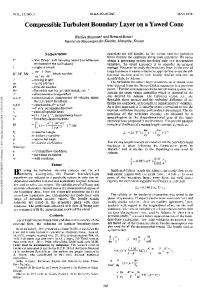
A two-dimensional spectra for boundary layer does not exist mathematically, since the only homogeneous direction is spanwise. Spectra is therefore computed as the Fourier transform of the two-points correlation function of each Fourier mode, after symmetrizing it with respect to x. The largest streamwise wavelength is chosen to be x ⇡ 20 99 for all the spectra, in which the boundary layer can be approximately considered as a parallel flow (for x ⇡ 20 99 , / ⇡ 0.25). + Figure 3(a) compares kinetic spectral density energy uu for channels at Re⌧ = 550 2000 and boundary layers at similar values of Re⌧ at the buffer layer, y + = 15 and for energy levels of 15% and 57% of the total energy. They clearly show the development of the scale separation with the Reynolds number, and also that the layers are slightly shorter than the channels at similar Re⌧ [Jiménez, Hoyas, Simens & Mizuno, 2010]. On the other hand, they show that the aspect ratio of the large structures in both flows are essentially the same, x = 10 z .

Figure 3. (a) Solid lines are two-dimensional spectral densities Φ+ uu from channels at Reτ = 550– 2000 [Hoyas & Jiménez, 2006], and dashed ones those of boundary layers at Reτ = 550 [Jiménez, Hoyas, Simens & Mizuno, 2010], and 1000 and 2000 from the present case at the buffer layer, y + = 15, in red, blue, and black respectively. (b) Large scales boundary layer footprint in the + vorticity spectral densities Φ+ ωω at the viscous sublayer y = 5 (black) and for the buffer layer + at y = 10 − 15 (red, blue) at Reτ ≈ 2000. In both cases, the straight dashed line is λx = 10λz and dots are λz = Reτ . It is interesting to note the effect of the Reynolds number near the wall, due to the large scale inactive motions in the sense of [Townsend, 1976]. This is clearly seen in figure 3(b), in which the spectral enstrophy density Φ+ ωω is presented for the boundary layer at Reτ ≈ 2000 at different wall-normal locations and for enstrophy levels of 8% and 50% of the total. Near the wall, the large scales of the flow are irrotational, because the v impermeability condition inhibits the Reynolds stresses hu0 v 0 i. This can be seen at the buffer layer locations, y + = 10 (red) and y + = 15 (blue), where the large scales are missing. The nearest wall value is y + = 5 (black), within the viscous layer, and in which the potential flow cannot satisfy the no-slip boundary condition, developing a thin rotational sublayer in which structures are long and wide so the no-slip condition is attained [Hoyas & Jiménez, 2008]. Very near to the wall the vorticity is the velocity gradient in the wall-normal direction, therefore, the vorticity and the velocity spectrum should be proportional at a constant y + , as observed in figure 3. 1D | versus y shows that the streamwise Further analysis of the one-dimensional spectra k|E∗∗ velocities fluctuations structures are long, those for spanwise wide, and those for wall-normal tall. The pressure fluctuations structures are as tall as the wall-normal velocity, but wider and slightly shorter than the streamwise fluctuations ones. This pattern can be observed in figure 5

13th European Turbulence Conference (ETC13) Journal of Physics: Conference Series 318 (2011) 022023

IOP Publishing doi:10.1088/1742-6596/318/2/022023

4, in which velocity fluctuations of an instantaneous realization of the flow field in the range Re✓ = 5800 6600 (Re⌧ ⇡ 1797 2016) are presented.

Figure 4. Instantaneous sections of the fluctuations: u+ (a, b), v + (c, d), w+ (e, f ), p+ (g, h). (a, c, e, g) are the x y sections for Re✓ = 5800 6600. (b, d, f, h) are the z y sections at Re✓ = 5800. Fluctuations are normalized with the friction velocity, and the coordinates are normalized with 99 at Re✓ = 5800. Dark grey areas are below -0.5 wall units, and lighter areas above +0.5.

4. Conclusions We have introduced the concept of the effective dimensionless length x ˜ in order to characterize the accommodation length needed for the large-scale structure of the flows to converge from artificial tripping methods to nominal values, resulting in lengths about x ˜ ⇡ 4. This is especially severe in the case of high Re✓ in which the flow may not achieve the equilibrium by the end of the physical domain. In order to perform a direct numerical simulation of a boundary layer at high Re✓ , an auxiliary simulation is conducted using relatively coarse resolution, and resolving correctly the large scales of the flow. The computational penalization of this auxiliary boundary layer is about 10% of the total time. It turns out that even at this low resolution the small scales are essentially well-resolved. A preliminary analysis of the statistics of this new simulation has been conducted. Integral parameters, such as cf and the shape factor, are within the scatter of the available experiments and numerical data sets. The same is true of the velocity fluctuations. At this relatively high Reynolds number, the mean profile exhibits a clear logarithmic region, and the fluctuations have been compared with the numerical channel at similar Reynolds numbers. Velocity fluctuations clearly show a weak dependence with the Re⌧ at the buffer layer, failing the classical scaling with the friction velocity u⌧ . The new simulation confirms that the transverse velocity fluctuations are stronger in boundary layers than in channels. Energy density spectra also shows the largescale structure footprint near the wall. Boundary layer and channel kinetic energy spectra are compared in that near-wall region, revealing that the structures for channels are somewhat larger than boundary layers, but showing similar features for the small-scale structures.

6

13th European Turbulence Conference (ETC13) Journal of Physics: Conference Series 318 (2011) 022023

IOP Publishing doi:10.1088/1742-6596/318/2/022023

Acknowledgments This research used resources of the Argonne Leadership Computing Facility at Argonne National Laboratory, which is supported by the Office of Science of the U.S. Department of Energy under contract DE-AC02-06CH11357. The work at the UPM was funded by CICYT under grant TRA2009-11498, and by the European Research Council under grant ERC-2010.AdG-20100224. J.A. Sillero was supported by an FPU fellowship from the UPM. References Lund, T. S., Wu, X. & Squires, K. D. 1998 Generation of Turbulent Inflow Data for SpatiallyDeveloping Boundary Layer Simulations. J. Comput. Phys. 140, 233–258 Hoyas, S. & Jiménez, J. 2006 Scaling of the velocity fluctuations in turbulent channels up to Re⌧ = 2003. Phys. Fluids 18, 011702 Jiménez, J., Hoyas, S., Simens, M. P. & Mizuno, Y. 2010 Turbulent boundary layers and channels at moderate Reynolds number. J. Fluid Mech. 657, 335–360 Jiménez, J. & Hoyas, S. 2008 Turbulent fluctuations above the buffer layer of wall-bounded flows. J. Fluid Mech. 611, 215–236 Jiménez, J., del Álamo, J. C. & Flores, O. 2004 The large-scale dynamics of near-wall turbulence. J. Fluid Mech. 505, 179–199 Simens, M. P., Jiménez, J., Hoyas, S. & Mizuno, Y. 2009 A high-resolution code for turbulent boundary layers. J. Comput. Phys. 228, 4218–4231 De Graaff, D. B. & Eaton, J. K. 2000 Reynolds number scaling of the flat-plate turbulent boundary layer. J. Fluid Mech. 422, 319–346 Osterlund, J. M., Johansson, A. V., Nagib, H. M. & Hites, M. 2000 A note on the overlap region in turbulent boundary layers. Phys. Fluids 12, 1–4 Schlatter, P. & Örlü, R. 2010 Assessment of direct numerical simulation data of turbulent boundary layers. J. Fluid Mech. 659, 116–126 Purtell, L. P., Klebanoff, P. S. & Buckley, F. T. 1981 Turbulent boundary layers at low Reynolds numbers. Phys. Fluids 24, 802–811 Erm, L. P. & Joubert, P. N. 1991 Low-Reynolds-number turbulent boundary layers. J. Fluid Mech. 230, 1–44 Hoyas, S. & Jiménez, J. 2008 Reynolds number effects on the Reynolds-stress budgets in turbulent channels. , Phys. Fluids 20, 101511 Townsend, A.A. 1976 The structure of turbulent shear flow. 2nd ed. (Cambridge U. Press, Cambridge)

7