2-approximation algorithm for the Student-Project Allocation problem

A 32 -approximation algorithm for the Student-Project Allocation problem Frances Cooper1 School of Computing Science, University of Glasgow [Glasgow, Scotland, UK] [email protected] [https://orcid.org/0000-0001-6363-9002]

David Manlove2

arXiv:1804.02731v1 [cs.DS] 8 Apr 2018

School of Computing Science, University of Glasgow [Glasgow, Scotland, UK] [email protected] [https://orcid.org/0000-0001-6754-7308]

Abstract The Student-Project Allocation problem with lecturer preferences over Students (spa-s) comprises three sets of agents, namely students, projects and lecturers, where students have preferences over projects and lecturers have preferences over students. In this scenario we seek a stable matching, that is, an assignment of students to projects such that there is no student and lecturer who have an incentive to deviate from their assignee/s. We study spa-st, the extension of spa-s in which the preference lists of students and lecturers need not be strictly ordered, and may contain ties. In this scenario, stable matchings may be of different sizes, and it is known that max spa-st, the problem of finding a maximum stable matching in spa-st, is NP-hard. We present a linear-time 32 -approximation algorithm for max spa-st and an Integer Programming (IP) model to solve max spa-st optimally. We compare the approximation algorithm with the IP model experimentally using randomly-generated data. We find that the performance of the approximation algorithm easily surpassed the 23 bound, constructing a stable matching within 92% of optimal in all cases, with the percentage being far higher for many instances. 2012 ACM Subject Classification Theory of computation → Design and analysis of algorithms Keywords and phrases Matching problems, Approximation, Algorithms, Stability Digital Object Identifier 10.4230/LIPIcs.SEA.2018.8

1

Introduction

Background and motivation. In universities all over the world, students need to be assigned to projects as part of their degree programmes. Lecturers typically offer a range of projects, and students may rank a subset of the available projects in preference order. Lecturers may have preferences over students, or over the projects they offer, or they may not have explicit preferences at all. There may also be capacity constraints on the maximum numbers of students that can be allocated to each project and lecturer. The problem of allocating students to projects subject to these preference and capacity constraints is called the Student-Project Allocation problem (spa) [8, Section 5.5][4, 5]. Variants of this problem can be defined for the cases that lecturers have preferences over the students that rank their

1 2

[Supported by an Engineering and Physical Sciences Research Council Doctoral Training Account] [Supported by Engineering and Physical Sciences Research Council grant EP/P028306/01]

© Frances Cooper and David Manlove; licensed under Creative Commons License CC-BY 17th International Symposium on Experimental Algorithms (SEA 2018). Editor: Gianlorenzo D’Angelo; Article No. 8; pp. 8:1–8:48 Leibniz International Proceedings in Informatics Schloss Dagstuhl – Leibniz-Zentrum für Informatik, Dagstuhl Publishing, Germany

8:2

A 32 -approximation algorithm for the Student-Project Allocation problem projects [2], or over the projects they offer [10], or not at all [7]. In this paper we focus on the first of these cases, where lecturers have preferences over students – the so-called Student-Project Allocation problem with lecturer preferences over Students (spa-s). Finding an optimal allocation of students to projects manually is time-consuming and errorprone. Consequently many universities automate the allocation process using a centralised algorithm. Given the typical sizes of problem instances (e.g., 130 students at the University of Glasgow, School of Computing Science), the efficiency of the matching algorithm is of paramount importance. In the case of spa-s, the desired matching must be stable with respect to the given preference lists, meaning that no student and lecturer have an incentive to deviate from the given allocation and form an assignment with one another [11]. Abraham et al. [2] described a linear-time algorithm to find a stable matching in an instance I of spa-s when all preference lists in I are strictly ordered. They also showed that, under this condition, all stable matchings in I are of the same size. In this paper we focus on the variant of spa-s in which preference lists of students and lecturers can contain ties, which we refer to as the Student-Project Allocation problem with lecturer preferences over Students including Ties (spa-st). Ties allow both students and lecturers to express indifference in their preference lists (in practice, for example, lecturers may be unable to distinguish between certain groups of students). A stable matching in an instance of spa-st can be found in linear time by breaking the ties arbitrarily and using the algorithm of Abraham et al. [2]. The Stable Marriage problem with Ties and Incomplete lists (smti) is a special case of spa-st in which each project and lecturer has capacity 1, and each lecturer offers one project. Given an instance of smti, it is known that stable matchings can have different sizes [9], and thus the same is true for spa-st. Yet in practical applications it is desirable to match as many students to projects as possible. This motivates max spa-st, the problem of finding a maximum (cardinality) stable matching in an instance of spa-st. This problem is NP-hard, since the corresponding optimisation problem restricted to smti, which we refer to as max smti, is NP-hard [9]. Király [6] described a 32 -approximation algorithm for max smti. He also showed how to extend this algorithm to the case of the Hospitals-Residents problem with Ties (hrt), where hrt is the special case of spa-st in which each lecturer l offers one project p, and the capacities of l and p are equal. Yanagisawa [12] showed that max smti is not approximable within a factor of 33 29 unless P=NP; the same bound applies to max spa-st. Our contribution. In this paper we describe a linear-time 32 -approximation algorithm for max spa-st. This algorithm is a non-trivial extension of Király’s approximation algorithm for hrt as mentioned above. We also describe an Integer Programming (IP) model to solve max spa-st optimally. Through a series of experiments on randomly-generated data, we then compare the sizes of stable matchings output by our approximation algorithm with the sizes of optimal solutions obtained from our IP model. Our main finding is that the performance of the approximation algorithm easily surpassed the 32 bound on the generated instances, constructing a stable matching within 92% of optimal in all cases, with the percentage being far higher for many instances. Note that a natural “cloning” technique, involving transforming an instance I of spa-st into an instance I 0 of smti, and then using Király’s 32 -approximation algorithm for smti [6] in order to obtain a similar approximation in spa-st, does not work in general, as we show in Appendix A. This motivates the need for a bespoke algorithm for the spa-st case. Structure of this paper. Section 2 gives a formal definition of spa-st. Section 3 describes the 32 -approximation algorithm, and the IP model for max spa-st is given in Section 4. The experimental evaluation is described in Section 5, and Section 6 discusses future work.

F. Cooper and D. Manlove

2

8:3

Formal definition of spa-st

An instance I of spa-st comprises a set S = {s1 , s2 , ..., sn1 } of students, a set P = {p1 , p2 , ..., pn2 } of projects, and a set L = {l1 , l2 , ..., ln3 } of lecturers. Each project is offered by one lecturer, and each lecturer lk offers a set of projects Pk ⊆ P , where P1 , . . . , Pk partitions P . Each project pj ∈ P has a capacity cj ∈ Z+ 0 , and similarly each lecturer lk ∈ L has a capacity dk ∈ Z+ 0 . Each student si ∈ S has a set Ai ⊆ P of acceptable projects that they rank in order of preference. Ties are allowed in preference lists, where a tie t in a student si ’s list indicates that si is indifferent between all projects in t. Each lecturer lk ∈ L has a preference list over the students si for which Ai ∩ Pk 6= ∅. Ties may also exist in lecturer preference lists. The rank of project pj on student si ’s list, denoted rank(si , pj ), is defined as 1 plus the number of projects that si strictly prefers to pj . An analogous definition exists for the rank of a student on a lecturer’s list, denoted rank(lk , si ). An assignment M in I is a subset of S × P such that, for each pair (si , pj ) ∈ M , pj ∈ Ai , that is, si finds pj acceptable. Let M (si ) denote the set of projects assigned to a student si ∈ S, let M (pj ) denote the set of students assigned to a project pj ∈ P , and let M (lk ) denote the set of students assigned to projects in Pk for a given lecturer lk ∈ L. A matching M is an assignment such that |M (si )| ≤ 1 for all si ∈ S, |M (pj )| ≤ cj for all pj ∈ P and |M (lk )| ≤ dk for all lk ∈ L. If si ∈ S is assigned in a matching M , we let M (si ) denote si ’s assigned project, otherwise M (si ) is empty. Given a matching M in I, let (si , pj ) ∈ (S × P )\M be a student-project pair, where pj is offered by lecturer lk . Then (si , pj ) is a blocking pair of M [2] if 1, 2 and 3 hold as follows: 1. si finds pj acceptable; 2. si either prefers pj to M (si ) or is unassigned in M ; 3. Either a, b or c holds as follows: a. pj is undersubscribed (i.e., |M (pj )| < cj ) and lk is undersubscribed (i.e., |M (lk )| < dk ); b. pj is undersubscribed, lk is full and either si ∈ M (lk ) or lk prefers si to the worst student in M (lk ); c. pj is full and lk prefers si to the worst student in M (pj ). Let (si , pj ) be a blocking pair of M . Then we say that (si , pj ) is of type (3x) if 1, 2 and 3x are true in the above definition, where x ∈ {a, b, c}. In order to more easily describe certain stages of the approximation algorithm, blocking pairs of type (3b) are split into two subtypes as follows. (3bi) defines a blocking pair of type (3b) where si is already assigned to another project of lk ’s. (3bii) defines a blocking pair of type (3b) where this is not the case. A matching M in an instance I of spa-st is stable if it admits no blocking pair. Define max spa-st to be the problem of finding a maximum stable matching in spa-st and let Mopt denote a maximum stable matching for a given instance. Similarly, let min spa-st be the problem of finding a minimum stable matching in spa-st.

3 3.1

Approximation algorithm Introduction and preliminary definitions

We begin by defining key terminology before describing the approximation algorithm itself in Section 3.2, which is a non-trivial extension of Király’s hrt algorithm [6]. A student si ∈ S is either in phase 1, 2 or 3. In phase 1 there are still projects on si ’s list that they have not applied to. In phase 2, si has iterated once through their list and are doing so again whilst a priority is given to si on each lecturer’s preference list, compared to

SEA 2018

8:4

A 32 -approximation algorithm for the Student-Project Allocation problem other students who tie with si . In phase 3, si is considered unassigned and carries out no more applications. A project pj is fully available if pj and lk are both undersubscribed, where lecturer lk offers pj . A student si meta-prefers project pj1 to pj2 if either (i) rank(si , pj1 ) < rank(si , pj2 ), or (ii) rank(si , pj1 ) = rank(si , pj2 ) and pj1 is fully available, whereas pj2 is not. In phase 1 or 2, si may be either available, provisionally assigned or confirmed. Student si is available if they are not assigned to a project. Student si is provisionally assigned if si has been assigned in phase 1 and there is a project still on si ’s list that meta-prefers to pj . Otherwise, si is confirmed. If a student si is a provisionally assigned to project pj , then (si , pj ) is said to be precarious. A project pj is precarious if it is assigned a student si such that (si , pj ) is precarious. A lecturer is precarious if they offer a project pj that is precarious. Lecturer lk meta-prefers si1 to si2 if either (i) rank(lk , si1 ) < rank(lk , si2 ), or (ii) rank(lk , si1 ) = rank(lk , si2 ) and si1 is in phase 2, whereas si2 is not. The favourite projects Fi of a student si are defined as the set of projects on si ’s preference list for which there is no other project on si ’s list meta-preferred to any project in Fi . A worst assignee of lecturer lk is defined to be a student in M (lk ) of worst rank, with priority given to phase 1 students over phase 2 students. Similarly, a worst assignee of lecturer lk in M (pj ) is defined to be a student in M (pj ) of worst rank, prioritising phase 1 over phase 2 students, where lk offers pj . We remark that some of the above terms such as favourite and precarious have been defined for the spa-st setting by extending the definitions of the corresponding terms as given by Király in the hrt context [6].

3.2

Description of the algorithm

Algorithm 1 begins with an empty matching M which will be built up over the course of the algorithm’s execution. All students are initially set to be available and in phase 1. The algorithm proceeds as follows. While there are still available students in phase 1 or 2, choose some such student si . Student si applies to a favourite project pj at the head of their list, that is, there is no project on si ’s list that si meta-prefers to pj . Let lk be the lecturer who offers pj . We consider the following cases. If pj and lk are both undersubscribed then (si , pj ) is added to M . Clearly if (si , pj ) were not added to M , it would potentially be a blocking pair of type (3a). If pj is undersubscribed, lk is full and lk is precarious where precarious pair (si0 , pj 0 ) ∈ M for some project p0j offered by lk , then we remove (si0 , pj 0 ) from M and add pair (si , pj ). This notion of precariousness allows us to find a stable matching of sufficient size even when there are ties in student preference lists (there may also be ties in lecturer preference lists). Allowing a pair (si0 , pj 0 ) ∈ M to be precarious means that we are noting that si0 has other fully available project options in their preference list at equal rank to pj 0 . Hence, if another student applies to pj 0 when pj 0 is full, or to a project offered by lk where lk is full, we allow this assignment to happen removing (si0 , pj 0 ) from M , since there is a chance that the size of the resultant matching could be increased. If on the other hand pj is undersubscribed, lk is full and lk meta-prefers si to a worst assignee si0 , where (si0 , pj 0 ) ∈ M for some project pj 0 offered by lk , then we remove (si0 , pj 0 ) from M and add pair (si , pj ). It makes intuitive sense that if lk is full and gets an offer to an undersubscribed project from a student si that they prefer to a worst assigned student si0 , then lk would want to remove si0 from pj 0 and take on si for pj 0 . Student si0 will subsequently remove pj 0 from their preference list as lk will not want to assign to them on re-application. This is done via the Remove-pref method (Algorithm 2).


8:5

Algorithm 1 3/2-approximation algorithm for spa-st Require: An instance I of spa-st Ensure: Return a stable matching M where |M | ≥ 23 |Mopt | 1: M ← ∅ 2: all students are initially set to be available and in phase 1 3: while there exists an available student si ∈ S who is in phase 1 or 2 do 4: let lk be the lecturer who offers pj 5: si applies to a favourite project pj ∈ A(si ) 6: if pj is fully available then 7: M ← M ∪ {(si , pj )} 8: else if pj is undersubscribed, lk is full and (lk is precarious or lk meta-prefers si to a worst assignee) then . according to the worst assignee definition in Section 3.1 9: if lk is precarious then let pj 0 be a project in Pk such that there exists (si0 , pj 0 ) ∈ M that is precarious 10: 11: else . lk is not precarious 12: let si0 be a worst assignee of lk such that lk meta-prefers si to si0 and let pj 0 = M (si0 ) 13: Remove-Pref(si0 , pj 0 ) 14: end if 15: M ← M \{(si0 , pj 0 )} 16: M ← M ∪ {(si , pj )} 17: else if pj is full and (pj is precarious or lk meta-prefers si to a worst assignee in M (pj )) then 18: if pj is precarious then 19: identify a student si0 ∈ M (pj ) such that (si0 , pj ) is precarious 20: else . pj is not precarious 21: let si0 be a worst assignee of lk in M (pj ) such that lk meta-prefers si to si0 22: Remove-Pref(si0 , pj ) 23: end if 24: M ← M \{(si0 , pj )} 25: M ← M ∪ {(si , pj )} 26: else 27: Remove-Pref(si , pj ) 28: end if 29: end while 30: Promote-students(M ) 31: return M ;

If pj is full and precarious then pair (si , pj ) is added to M while precarious pair (si0 , pj ) is removed. As before, this allows si0 to potentially assign to other fully available projects at the same rank as pj on their list. Since si0 does not remove pj from their preference list, si0 will get another chance to assign to pj if these other applications to fully available projects at the same rank are not successful. If pj is full and lk meta-prefers si to a worst assignee si0 in M (pj ), then pair (si , pj ) is added to M while (si0 , pj ) is removed. As this lecturer’s project is full (and not precarious) the only time they will want to add a student si to this project (meaning the removal of another student) is if si is preferred to a worst student si0 assigned to that project.

SEA 2018

8:6

A 32 -approximation algorithm for the Student-Project Allocation problem

Algorithm 2 Remove-Pref(si , pj ) – remove a project from a student’s preference list Require: An instance I of spa-st and a student si and project pj Ensure: Return an instance I where pj is removed from si ’s preference list 1: remove pj from si ’s preference list 2: if si ’s preference list is empty then 3: reinstate si ’s preference list 4: if si is in phase 1 then 5: move si to phase 2 6: else if si is in phase 2 then 7: move si to phase 3 8: end if 9: end if 10: return instance I Algorithm 3 Promote-students(M ) – remove all blocking pairs of type (3bi) Require: SPA-ST instance I and matching M that does not contain blocking pairs of type (3a), (3bii) or (3c). Ensure: Return a stable matching M . 1: while there are still blocking pairs of type (3bi) do 2: Let (si , pj 0 ) be a blocking pair of type (3bi) 3: M ← M \{(si , M (si ))} 4: M ← M ∪ {(si , pj 0 )} 5: end while 6: return M Similar to before, si0 will not subsequently be able to assign to this project and so removes it from their preference list via the Remove-pref method (Algorithm 2). When removing a project from a student si ’s preference list (the Remove-pref operation of Algorithm 2), if si has removed all projects from their preference list and is in phase 1 then their preference list is reinstated and they are set to be in phase 2. If on the other hand they were already in phase 2, then they are set to be in phase 3 and are hence inactive. The proof that Algorithm 1 produces a stable matching (see Appendix B) relies only on the fact that a student iterates once through their preference list. Allowing students to iterate through their preference lists a second time when in phase 2 allows us to find a stable matching of sufficient size when there are ties in lecturer preference lists (there may also be ties in student preference lists). This is due to the meta-prefers definition where a lecturer favours one student si over another si0 if they are the same rank and si is in phase 2 whereas si0 is not. Similar to above, this then allows si to steal a position from si0 with the chance that si0 may find another assignment and increase the size of the resultant matching. After the main while loop has terminated, the final part of the algorithm begins where all blocking pairs of type (3bi) are removed using the Promote-students method (Algorithm 3).

3.3

Proof of correctness

I Theorem 1. Let M be a matching found by Algorithm 1 for an instance I of spa-st. Then M is stable and |M | ≥ 23 |Mopt |, where Mopt is a maximum stable matching in I. Proof. Theorems 18, 22 and Theorem 30, proved in Appendix B, show that M is stable, and


8:7

that Algorithm 1 runs in polynomial time and has performance guarantee 32 . The proofs required for this algorithm are naturally longer and more complex than given by Király [6] for smti, as spa-st generalises smti to the case that lecturers can offer multiple projects, and projects and lecturers may have capacities greater than 1. These extensions add extra components to the definition of a blocking pair (given in Section 2) which in turn adds complexity to the algorithm and its proof of correctness. J Appendix B.5 shows a simple example instance where a matching found by Algorithm 1 is exactly 23 times the optimal size, hence the analysis of the performance guarantee is tight.

4

IP model

In this section we present an IP model for max spa-st. For the stability constraints in the model, it is advantageous to use an equivalent condition for stability, as given by the following lemma, whose proof can be found in Appendix C. I Lemma 2. Let I be an instance of SPA-ST and let M be a matching in I. Then M is stable if and only if the following condition, referred to as condition (*) holds: For each student si ∈ S and project pj ∈ P , if si is unassigned in M and finds pj acceptable, or si prefers pj to M (si ), then either: lk is full, si ∈ / M (lk ) and lk prefers the worst student in M (lk ) to si or is indifferent between them, or; pj is full and lk prefers the worst student in M (pj ) to si or is indifferent between them, where lk is the lecturer offering pj . The key variables in the model are binary-valued variables xij , defined for each si ∈ S and pj ∈ P , where xij = 1 if and only if student si is assigned to project pj . Additionally, we have binary-valued variables αij and βij for each si ∈ S and pj ∈ P . These variables allow us to more easily describe the stability constraints below. For each si ∈ S and lk ∈ L, let Tik = {su ∈ S : rank(lk , su ) ≤ rank(lk , si ) ∧ su 6= si }. That is, Tik is the set of students ranked at least as highly as student si in lecturer lk ’s preference list not including si . Also, for each pj ∈ P , let Tijk = {su ∈ S : rank(lk , su ) ≤ rank(lk , si ) ∧ su 6= si ∧ pj ∈ A(su )}. That is, Tijk is the set of students su ranked at least as highly as student si in lecturer lk ’s preference list, such that project pj is acceptable to su , not including si . Finally, let Sij = {pr ∈ P : rank(si , pr ) ≤ rank(si , pj )}, that is, Sij is the set of projects ranked at least as highly as project pj in student si ’s preference list, including pj . Figure 1 shows the IP model for max spa-st. Equation (1) enforces xij = 0 if si finds pj unacceptable. Inequality (2) ensures that a student may be assigned to a maximum of one project. Inequalities (3) and (4) ensure that project and lecturer capacities are enforced. In the left hand side of Inequality (5), if P 1 − pr ∈Sij xir = 1, then either si is unmatched or si prefers pj to M (si ). This also ensures that either αij = 1 or βij = 1, described in Inequalities (6) and (7). Inequality (6) ensures that, if αij = 1, the number of students ranked at least as highly as student si by lk (not including si ) and assigned to lk must be at least lk ’s capacity dk . Inequality (7) ensures that, if βij = 1, the number of students ranked at least as highly as student si in lecturer lk ’s preference list (not including si ) and assigned to pj must be at least pj ’s capacity cj .

SEA 2018

8:8


X X

maximise:

xij

si ∈S pj ∈P

subject to: 1. xij = 0 X 2. xij ≤ 1

∀si ∈ S ∀pj ∈ P , pj ∈ / A(si ) ∀si ∈ S

pj ∈P

3.

X

xij ≤ cj

∀pj ∈ P

si ∈S

4.

X X

xij ≤ dk

∀lk ∈ L

si ∈S pj ∈Pk

5.

X

1−

xir ≤ αij + βij

∀si ∈ S ∀pj ∈ P

pr ∈Sij

6.

X

X

xur ≥ dk αij


su ∈Tik pr ∈Pk

7.

X

xuj ≥ cj βij


su ∈Tijk

xij ∈ {0, 1},

αij ∈ {0, 1},

βij ∈ {0, 1}


Figure 1 IP model for max spa-st.

Finally, for our optimisation we maximise the sum of all xij variables in order to maximise the number of students assigned. The following result, proved in Appendix C, establishes the correctness of the IP model. I Theorem 3. Given an instance I of spa-st, let J be the IP model as defined in Figure 1. A maximum stable matching in I corresponds to an optimal solution in J and vice versa.

5 5.1

Experimental evaluation Methodology

Experiments were conducted on the approximation algorithm and the IP model using randomly-generated data in order to measure the effects on matching statistics when changing parameter values relating to (1) instance size, (2) probability of ties in preference lists, and (3) preference list lengths. Two further experiments (referred to as (4) and (5) below) explored scalability properties for both techniques. Instances were generated using both existing and new software. The existing software is known as the Matching Algorithm Toolkit and is a collaborative project developed by students and staff at the University of Glasgow. For a given spa-st instance, let the total project and lecturer capacities be denoted by cP and dL , respectively. Note that these capacities were distributed randomly, subject to there being a maximum difference of 1 between the capacities of any two projects or any two lecturers (to ensure uniformity). The minimum and maximum size of student preference lists is given by lmin and lmax , and ts represents the probability that a project on a student’s preference list is tied with the next project. Lecturer preference lists were generated initially from the student preference lists, where a lecturer lk must rank a student if a student ranks


8:9

a project offered by lk . These lists were randomly shuffled and tl denotes the ties probability for lecturer preference lists. A linear distribution was used to make some projects more popular than others and in all experiments the most popular project is around 5 times more popular than the least. This distribution influenced the likelihood of a student finding a given project acceptable. Parameter details for each experiment are given below. (1) Increasing instance size: 10 sets of 10, 000 instances were created (labelled SIZE1, ..., SIZE10). The number of students n1 increased from 100 to 1000 in steps of 100, with n2 = 0.6n1 , n3 = 0.4n1 , cP = 1.4n1 , dL = 1.2n1 . The probabilities of ties in preference lists were ts = tl = 0.2 throughout all instance sets. Lengths of preference lists lmin = 3 and lmax = 5 also remained the same and were kept low to ensure a wide variability in stable matching size per instance. (2) Increasing probability of ties: 11 sets of 10, 000 instances were created (labelled TIES1, ..., TIES11). Throughout all instance sets n1 = 300, n2 = 250, n3 = 120, cP = 420, dL = 360, lmin = 3 and lmax = 5. The probabilities of ties in student and lecturer preference lists increased from ts = tl = 0.0 to ts = tl = 0.5 in steps of 0.05. (3) Increasing preference list lengths: 10 sets of 10, 000 instances were generated (labelled PREF1, ..., PREF10). Similar to the TIES cases, throughout all instance sets n1 = 300, n2 = 250, n3 = 120, cP = 420 and dL = 360. Additionally, ts = tl = 0.2. Preference list lengths increased from lmin = lmax = 1 to lmin = lmax = 10 in steps of 1. (4) Instance size scalability: 5 sets of 10 instances were generated (labelled SCALS1, ..., SCALS5). All instance sets in this experiment used the same parameter values as the SIZE experiment, except the number of students n1 increased from 10, 000 to 50, 000 in steps of 10, 000. (5) Preference list scalability: Finally, 6 sets of 10 instances were created (labelled SCALP1, ..., SCALP6). Throughout all instance sets n1 = 500 with the same values for other parameters as the SIZE experiment. However in this case ties were fixed at ts = tl = 0.4, and lmin = lmax increasing from 25 to 150 in steps of 25. For each generated instance, we ran the 32 -approximation algorithm and then used the IP model to find a maximum stable matching. We also computed a minimum stable matching using a simple adaptation of our IP model for max spa-st, in order to measure the spread in the sizes of stable matchings. A timeout of 1800 seconds (30 minutes) was imposed on all instance runs. All experiments were conducted using a machine with 32 cores, 8×64GB RAM and Dual Intel® Xeon® CPU E5-2697A v4 processors. The operating system was Ubuntu version 17.04 with all code compiled in Java version 1.8, where the IP models were solved using Gurobi version 7.5.2. Each approximation algorithm instance was run on a single thread while each IP instance was run on two threads. No attempt was made to parallelise Java garbage collection. Repositories for the code and data can be found at https://doi.org/ 10.5281/zenodo.1183221 and https://doi.org/10.5281/zenodo.1186823 respectively. Correctness testing was conducted over all generated instances. This consisted of (1) ensuring that each matching produced by the approximation algorithm was at least 23 the size of maximum stable matching, as found by the IP, and, (2) testing that a given allocation was stable and adhered to all project and lecturer capacities. This was run over all output from both the approximation algorithm and the IP-based algorithm.

5.2

Experimental results

Experimental results can be seen in Tables 1, 2, 3 and 4. Tables 1, 2 and 3 show the results from Experiments 1, 2 and 3 respectively (in which the instance size, probability of

SEA 2018

8:10

A 32 -approximation algorithm for the Student-Project Allocation problem ties and preference list lengths were increased, respectively). From this point onwards an optimal matching refers to a maximum stable matching. In these tables, column ‘minimum A/Max’ gives the minimum ratio of approximation algorithm matching size to optimal matching size that occurred, ‘% A=Max’ displays the percentage of times the approximation algorithm achieved an optimal result, and ‘% A≥ 0.98Max’ shows the percentage of times the approximation algorithm achieved a result at least 98% of optimal. The ‘average size’ columns are somewhat self explanatory, with sub-columns ‘A/Max’ and ‘Min/Max’ showing the average approximation algorithm matching size and minimum stable matching size as a fraction of optimal. Finally, ‘average total time’ indicates the time taken for model creation, solving and outputting results per instance. The main findings are summarised below. The approximation algorithm consistently far exceeds its 32 bound. Considering the column labelled ‘minimum A/Max’ in Tables 1, 2 and 3, we see that the smallest value was within the SIZE1 instance set with a ratio of 0.9286. This is well above the required bound of 23 . On average the approximation algorithm provides results that are closer in size to the average maximum stable matching than the minimum stable matching. The columns ‘A/Max’ and ‘Min/Max’ show that, on average, for each instance set, the approximation algorithm produces a solution that is within 98% of maximum and far closer to the maximum size than to the minimum size. Table 4 shows the scalability results for increasing instance sizes (Experiment 4) and increasing preference list lengths (Experiment 5). The ‘instances completed’ column indicates the number of instances completed before timeout occurred. In addition to showing the average total time taken (where ‘total’ includes model creation time and solution time), the column ‘average solve time’ displays the time taken to either execute the approximation algorithm, or solve the IP model (in both cases, model creation time is excluded). For Experiment 4, the number of instances solved within the 30-minute timeout reduced from 10 to 0 for the IP-based algorithm finding the maximum stable matching. However, even for the largest instance set sizes the approximation algorithm was able to solve all instances on average within a total of 21 seconds (0.8 seconds of which was used to actually execute the algorithm). For Experiment 5, with a higher probability of ties and increasing preference list lengths, the IP-based algorithm was only able to solve all the instances of one instance set (SCALP2) within 30 minutes each, however the approximation algorithm took less than 0.3 seconds on average to return a solution for each instance. This shows that the approximation algorithm is useful for either larger or more complex instances than the IP-based algorithm can handle, motivating its use for real world scenarios.

6

Future work

This paper has described a 32 -approximation algorithm for max spa-st. It remains open to describe an approximation algorithm that has a better performance guarantee, and/or to prove a stronger lower bound on the inapproximability of the problem than the current best bound of 33 29 [12]. Further experiments could also measure the extent to which the order that students apply to projects in Algorithm 1 affects the size of the stable matching generated. The work in this paper has mainly focused on the size of stable matchings. However, it is possible for a stable matching to admit a blocking coalition, where a permutation of student assignments could improve the allocations of the students and lecturers involved without harming anyone else. Since permutations of this kind cannot change the size of the matching they are not studied further here, but would be of interest for future work.

minimum A/Max

% A=Max

% A≥ 0.98Max

0.9286 0.9585 0.9556 0.9644 0.9654 0.9641 0.9679 0.9684 0.9653 0.9701

17.8 1.6 0.1 0.0 0.0 0.0 0.0 0.0 0.0 0.0

62.7 62.6 63.7 65.6 66.5 66.8 65.4 67.4 68.6 68.0

A 96.4 192.6 288.7 384.9 481.0 577.2 673.3 769.5 865.6 961.7

Min 92.0 183.4 274.9 366.4 457.7 549.3 640.5 732.0 823.4 914.7

average Max 97.8 195.7 293.7 391.7 489.6 587.7 685.7 783.8 881.7 979.7

size A/Max 0.986 0.984 0.983 0.983 0.982 0.982 0.982 0.982 0.982 0.982

Min/Max 0.941 0.937 0.936 0.935 0.935 0.935 0.934 0.934 0.934 0.934

average total time A Min 43.3 147.6 51.2 230.6 56.6 346.4 59.7 488.7 62.8 660.3 66.4 862.3 69.8 1127.8 73.0 1437.3 76.5 1784.3 86.6 2281.2

(ms) Max 137.8 210.6 313.4 429.3 555.6 713.0 900.6 1098.2 1343.9 1651.0

A 284.0 284.9 285.9 287.0 288.0 289.2 290.3 291.4 292.5 293.7 294.8

Min 284.0 282.0 279.9 277.6 275.1 272.4 269.4 266.2 262.7 258.9 254.8

average Max 284.0 285.8 287.9 289.9 291.9 294.0 295.7 297.2 298.3 299.1 299.5

size A/Max 1.000 0.997 0.993 0.990 0.986 0.984 0.982 0.980 0.980 0.982 0.984

Min/Max 1.000 0.987 0.972 0.958 0.942 0.927 0.911 0.896 0.880 0.866 0.851

average total time A Min 59.2 184.0 61.2 192.4 61.7 201.0 62.3 213.3 62.9 234.3 64.2 274.2 64.3 358.3 64.2 577.3 65.2 1234.1 59.6 2903.4 60.4 5756.9

(ms) Max 186.9 194.7 203.1 214.5 231.0 260.6 311.3 380.7 427.5 409.1 377.4


Case SIZE1 SIZE2 SIZE3 SIZE4 SIZE5 SIZE6 SIZE7 SIZE8 SIZE9 SIZE10

Table 1 Increasing instance size experimental results.

Case TIES1 TIES2 TIES3 TIES4 TIES5 TIES6 TIES7 TIES8 TIES9 TIES10 TIES11

minimum A/Max

% A=Max

% A≥ 0.98Max

1.0000 0.9792 0.9722 0.9655 0.9626 0.9558 0.9486 0.9527 0.9467 0.9529 0.9467

100.0 38.0 12.1 3.4 1.0 0.4 0.2 0.2 0.2 0.5 1.0

100.0 100.0 99.3 95.2 82.5 66.7 52.9 46.4 50.4 61.9 74.2

Table 2 Increasing probability of ties experimental results.

8:11

SEA 2018

8:12

minimum A/Max

% A=Max

% A≥ 0.98Max

1.0000 0.9699 0.9617 0.9623 0.9661 0.9732 0.9767 0.9833 0.9866 0.9900

100.0 12.3 1.2 1.0 4.2 15.7 36.2 58.2 75.5 87.3

100.0 99.0 84.0 82.8 95.1 99.5 100.0 100.0 100.0 100.0

A 215.0 262.1 280.9 290.0 294.8 297.3 298.7 299.3 299.7 299.8

Min 215.0 249.1 266.4 277.0 283.9 288.7 292.1 294.4 296.1 297.4

average Max 215.0 264.1 284.7 293.9 297.7 299.1 299.7 299.9 299.9 300.0

size A/Max 1.000 0.993 0.987 0.987 0.990 0.994 0.997 0.998 0.999 1.000

Min/Max 1.000 0.943 0.936 0.943 0.954 0.965 0.975 0.982 0.987 0.991

average total time A Min 74.3 107.5 67.5 133.8 68.1 181.4 69.1 249.7 68.3 346.7 66.1 472.4 64.5 638.3 64.1 811.9 63.4 1032.2 104.3 1239.4

Table 3 Increasing preference list length experimental results.

Case SCALS1 SCALS2 SCALS3 SCALS4 SCALS5 SCALP1 SCALP2 SCALP3 SCALP4 SCALP5 SCALP6

A 10 10 10 10 10 10 10 10 10 10 10

instances completed Min Max 10 10 10 9 10 0 7 0 7 0 0 9 1 10 0 3 0 1 0 0 0 0

Table 4 Scalability experimental results.

A 136.5 242.4 491.7 718.8 803.5 25.1 23.3 31.7 37.8 59.0 45.7

average solve time (ms) Min Max 126162.8 225917.9 348849.4 1091424.2 777267.7 N/A 1049122.0 N/A 1288961.1 N/A N/A 93086.0 1425177.0 626774.9 N/A 867107.7 N/A 1551376.0 N/A N/A N/A N/A

A 1393.8 5356.7 13095.3 18883.5 20993.0 193.3 189.4 196.6 248.5 283.7 288.4

average total time Min 127980.3 353272.3 785421.2 1062076.4 1307728.7 N/A 1428844.0 N/A N/A N/A N/A

(ms) Max 227764.3 1096045.6 N/A N/A N/A 94242.9 631225.2 882251.0 1594201.0 N/A N/A

(ms) Max 105.1 128.7 174.0 242.6 340.3 440.6 550.9 660.3 789.1 931.0


Case PREF1 PREF2 PREF3 PREF4 PREF5 PREF6 PREF7 PREF8 PREF9 PREF10


8:13

References 1

2 3 4

5 6 7

8 9 10 11 12

D.J. Abraham, K. Cechlárová, D.F. Manlove, and Kurt Melhorn. Pareto optimality in house allocation problems. In Proceedings. ISAAC ’04: The 15th Annual International Symposium on Algorithms and Computation, Lecture Notes in Computer Science, volume 3341, pages 3 – 15. Springer, 2004. D.J. Abraham, R.W. Irving, and D.F. Manlove. Two algorithms for the student-project allocation problem. Journal of Discrete Algorithms, 5:73–90, 2007. G. Brassard and P. Bratley. Fundamentals of Algorithmics. Prentice-Hall, 1996. R. Calvo-Serrano, G. Guillén-Gosálbez, S. Kohn, and A. Masters. Mathematical programming approach for optimally allocating students’ projects to academics in large cohorts. Education for Chemical Engineers, 20:11–21, 2017. M. Chiarandini, R. Fagerberg, and S. Gualandi. Handling preferences in student-project allocation. Annals of Operations Research, to appear, 2018. Z. Király. Linear time local approximation for maximum stable marriage. Algorithms, 6:471–484, 2013. A. Kwanashie, R.W. Irving, D.F. Manlove, and C.T.S. Sng. Profile-based optimal matchings in the Student–Project Allocation problem. In Proceedings of IWOCA ’14: the 25th International Workshop on Combinatorial Algorithms, volume 8986 of Lecture Notes in Computer Science, pages 213–225. Springer, 2015. D.F. Manlove. Algorithmics of Matching Under Preferences. World Scientific, 2013. D.F. Manlove, R.W. Irving, K. Iwama, S. Miyazaki, and Y. Morita. Hard variants of stable marriage. Theoretical Computer Science, 276(1-2):261–279, 2002. D.F. Manlove and G. O’Malley. Student-project allocation with preferences over projects. Journal of Discrete Algorithms, 6:553–560, 2008. A.E. Roth. The evolution of the labor market for medical interns and residents: a case study in game theory. Journal of Political Economy, 92(6):991–1016, 1984. H. Yanagisawa. Approximation Algorithms for Stable Marriage Problems. PhD thesis, Kyoto University, School of Informatics, 2007.

Appendix A

Cloning from SPA-ST to HRT

Manlove [8, Theorem 3.11] describes a polynomial transformation from a weakly stable matching in and instance of hrt to a weakly stable matching in an instance of smti, and vice versa, where the size of matchings is conserved. A natural cloning method to convert instances of SPA-ST to instances of HRT is given as Algorithm 4. This algorithm involves converting students into residents and projects into hospitals. Hospitals inherit their capacity from projects. Residents inherit their preference lists naturally from students. Hospitals inherit their preference lists from the lecturer who offers their associated project; a resident entry ri is ranked only if ri also ranks this hospital. In order to translate lecturer capacities into the HRT instance, a number of dummy residents are created for each lecturer. The number created for lecturer lk is equal to the sum of capacities of their offered projects Pk minus the capacity of lk . We will ensure that all dummy residents are assigned in any stable matching. To this end, each dummy resident has a first position tie of all hospitals associated with projects of lk , and each hospital hj in this set has a first position tie of all dummy residents associated with lk . In this way, as all dummy

SEA 2018

8:14

A 32 -approximation algorithm for the Student-Project Allocation problem residents must be assigned in any stable matching by Proposition 4 lecturer capacities are automatically adhered to. I Proposition 4. Let I 0 be an instance of hrt created from an instance I of spa-st using Algorithm 4. All dummy residents must be assigned in any stable matching in I 0 . Proof. In I 0 , for each lecturer lk , the number of dummy residents created is equal to P fk = pj ∈Pk cj − dk . Assume for contradiction that one of the dummy residents rdk1 is unassigned in some stable matching M 0 of I 0 . Let Hk denote the set of hospitals associated with projects of lk . Since rdk1 is a dummy resident, it must have all hospitals in Hk tied in first position. Also, each hospital in Hk must rank all fk dummy students (associated with lk ) in tied first position. Since rdk1 is unassigned in M 0 , rdk1 would prefer to be assigned to any hospital in Hk . Also, since there is at least one dummy resident unassigned, there must be at least one hospital hkd2 in Hk that has fewer first-choice assignees than its capacity. Hospital hkd2 must exist since if it did not, then all dummy residents would be matched. But then (rdk1 , hd2 ) would be a blocking pair of M 0 , a contradiction. J Algorithm 4 Clone-spa-st, Converts an spa-st instance into an HRT instance Require: An instance I of spa-st Ensure: Return an instance I 0 of hrt 1: for all student si in S do 2: create a resident ri 3: ri inherits their preference list from si ’s list, ranking hospitals rather than projects 4: end for 5: for all project pj in P do 6: create a hospital hj 7: hj ’s capacity is given by ej = cj 8: let lk be the lecturer offering project pj 9: hj inherits their preference list from lk ’s list, where a resident entry ri is retained only if ri also ranks hj 10: end for 11: for all lecturer lk in L do P 12: if dk < pj ∈Pk cj then P 13: let fk = pj ∈Pk cj − dk 14: create fk new dummy residents rk = {r1k , r2k , . . . , rfk } 15: let Hk denote the set of all hospitals in I 0 associated with the projects of Pk in I 16: the preference list of each dummy resident is given by a first position tie of all hospitals in Hk 17: a first position tie of all residents in rk is added to the start of the preference list of each hospital in Hk 18: end if 19: end for 20: Let hrt instance I 0 be formed from all residents (including dummy residents) and hospitals 21: return instance I 0 I Theorem 5. Given an instance I of spa-st we can construct an instance I 0 of hrt in O(n1 + Dn2 + m) time with the property that a stable matching M in I can be converted to a


8:15

P P stable matching M 0 in hrt in O(Dn2 + m) time, where |M 0 | = |M | + lk ∈Q pr ∈Pk (cr ) − dk . Here, n1 denotes the number of students, n2 the number of projects, D the total capacities of lecturers and m the total length of student preference lists. Proof. Suppose M is a stable matching in I. We construct an instance I 0 of hrt using Algorithm 4. The time complexity of O(n1 + Dn2 + m) for the reduction carried out by the algorithm is achieved by noting that I 0 has a maximum of n1 + n2 + D agents and that there are a maximum of Dn2 + m acceptable resident-hospital pairs. Initially let M 0 = M . Let the set of dummy residents Rd in I 0 form a resident-complete matching (when considering the residents in Rd ) with the set of all hospitals and add these pairs to M 0 . This is possible (as proved in Proposition 4) because for each lecturer lk each dummy resident associated with lk denoted Rdk finds all projects in Pk acceptable, and moreover the total number of remaining positions of the projects is at least as large as P pr ∈Pk (cr ) − |M (lk )| = δk and |Rk | = δk by definition. We claim that M 0 is stable in I 0 . Suppose for contradiction that (ri , hj ) blocks M 0 in I 0 . All dummy residents must be assigned in M 0 to their first-choice hospital by above, hence ri corresponds to a student si in I. Resident ri inherited their preference list from si hence we know that si finds pj acceptable. Therefore by the definition given in Section 2, condition (1) of a blocking pair of M in I is satisfied. Resident ri is either unassigned in M 0 or prefers hj to M 0 (ri ). Student si is therefore in an equivalent position and condition (2) of a blocking pair of M in I is satisfied. Hospital hj is either undersubscribed or prefers ri to their worst assignee in M 0 . If hj is undersubscribed, then pj must also be undersubscribed. If lk were full in M , P then hj would be full in M 0 since pr ∈Pk (cr ) = δk + |M (lk )| in this scenario, therefore lk must be undersubscribed. But if lk is undersubscribed then this satisfies condition (3a) of a blocking pair. If hj prefers ri to their worst assignee in M 0 , then lk must prefer si to their worst assignee in M (pj ). This satisfies condition 3(c) of a blocking pair. Therefore by the definition in Section 2, (si , pj ) is a blocking pair of M in I, a contradiction. Since dummy residents are added in the algorithm’s execution it is clear that in general |M | 6= |M 0 |. However, since all dummy residents must be assigned by Proposition 4, it is trivial to calculate the difference X X |M 0 | = |M | + |Rd | = |M | + (cr ) − dk . lk ∈Q pr ∈Pk

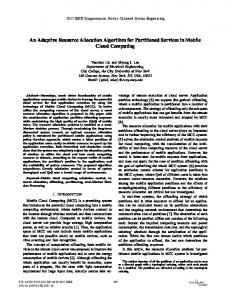
J The converse of Theorem 5 is not true in general, as shown in the example in Figure 2. Here a stable matching M 0 in an instance I 0 of hrt does not convert into a stable matching M of the associated instance I of spa-st. A natural question arises as to whether in special circumstances we can use the cloning process described in Algorithm 4: that is, convert to hrt then to smti, then use Király’s 3/2-approximation algorithm on the smti instance, and obtain as a result a matching that is a 3/2-approximation to a maximum stable matching in the original instance of spa-st. For example, assuming that the matching M resulting from the above process is stable, can we ensure the 3/2 bound? The following example demonstrates Algorithm 4 in use and shows that the process described above is not sufficient to retain the 3/2-approximation in an spa-st instance even if M is stable.

SEA 2018

8:16

A 32 -approximation algorithm for the Student-Project Allocation problem Resident preferences: r1 : h1 h2 r2 : h2 h3 r3 : (h1 h2 ) Hospital preferences: h1 : r3 r1 e1 = 1 h2 : r3 r2 r1 e2 = 1 h3 : r2 e3 = 1

Student preferences: s1 : p1 p2 s2 : p2 p3 Project details: p1 : lecturer l1 , c1 = 1 p2 : lecturer l1 , c2 = 1 p3 : lecturer l2 , c3 = 1 Lecturer preferences: l1 : s2 s1 d1 = 1 l2 : s2 d2 = 1

(a) hrt instance I0 converted from the spa-st instance in Figure 2b Stable matching M0 = {(r1 , h1 ), (r2 , h3 ), (r3 , h2 )} shown in bold.

(b) Example SPA-ST instance I. Unstable matching M = {(s1 , p1 ), (s2 , p3 )} derived from M 0 shown in bold.

Figure 2 Conversion of a stable matching M 0 in hrt into matching M in spa-st.

Algorithm 4 is used to convert the spa-st instance I in Figure 3a to an instance I 0 of HRT in Figure 3b which is then itself converted to the instance I 00 of SMTI in Figure 3c using the process described by Manlove [8, Theorem 3.11]. In this process men correspond to hospitals in I 0 (projects in I) and women correspond to residents in I 0 (students in I). Executing Király’s [6] 3/2-approximation algorithm on the smti instance I 00 could (depending on order of proposals) yield the matching M 00 = {(w2 , m4 ), (w4 , m3 ), (w5 , m2 ), (w6 , m6 ), (w7 , m7 )} in I 00 . A trace of how this matching is created is given in Table 5. As w5 , w6 and w7 were created from dummy residents in Algorithm 4, M 00 (stable in I 00 ) converts into the matching Mc = {(s2 , p4 ), (s4 , p3 )} of size 2 in I. But a maximum stable matching in I is of size 4, given by M = {(s1 , p3 ), (s2 , p1 ), (s3 , p3 ), (s4 , p2 )}. Therefore using the cloning method described above and Király’s algorithm does not result in a 3/2-approximation to the maximum stable matching for instances of spa-st. This motivates the development of a 3/2-approximation algorithm to the maximum stable matching specifically for instances of spa-st. An intuitive idea as to how the addition of dummy residents in the conversion of this spa-st instance to an smti instance stops the retention of the 3/2 bound follows. Figure 4a shows the spa-st instance I2 which is the same as the instance in Figure 3a but with project 1 and 2 capacities reduced to 1. Figure 4c shows I2 converted into an smti instance I200 using the same two-stage process as in Figure 3. Finally, Table 6 shows the algorithm trace for instance I200 using Király’s 3/2 smti algorithm. The main first difference in the traces can be seen on line 14 of Table 5 and line 11 of Table 6. On line 11 of Table 6, m2 applies to w4 as an advantaged man, giving them the ability to take w4 from m3 . This shows the benefit of having a tie including m2 and m3 at the beginning of w4 ’s list - either of these men being matched to w4 would be equally useful in a stable matching. Therefore allowing m2 to take w4 from m3 gives m3 a chance to get another partner, increasing the size of matching eventually attained. On line 14 of Table 5, m2 becomes ‘stuck’ on w5 , one of the women derived from a dummy resident. This stops m2


1 2 3 4 5 6 7 8 9 10 11 12 13 14 15 16 17 18 19 20 21 22 23 24 25 26 27 28 29 30 31 32 33 34 35 36 37 38 39

Action m7 applies w7 , accepted m6 applies w5 , accepted m5 applies w6 , accepted m4 applies w7 , rejected, w7 pref removed by m4 m4 applies w4 , accepted m3 applies w7 , rejected, w7 pref removed by m3 m3 applies w4 , accepted, w4 pref removed by m4 m4 applies w2 , accepted m2 applies w5 , rejected, w5 pref removed by m2 m2 applies w6 , rejected, w6 pref removed by m2 m2 applies w2 , rejected, w2 pref removed by m2 m2 applies w4 , rejected, w4 pref removed by m2 m2 advantaged m2 applies w5 , accepted, w5 removed by m6 m6 applies w6 , rejected, w6 removed by m6 m6 applies w2 , rejected, w2 removed by m6 m6 applies w4 , rejected, w4 removed by m6 m6 advantaged m6 applies w5 , rejected, w5 pref removed by m6 m6 applies w6 , accepted, w6 pref removed by m5 m5 applies w5 , rejected, w5 pref removed by m5 m5 applies w2 , rejected, w2 pref removed by m5 m5 applies w4 , rejected, w4 pref removed by m5 m5 advantaged m5 applies w5 , rejected, w5 pref removed by m5 m5 applies w6 , rejected, w6 pref removed by m5 m5 applies w2 , rejected, w2 pref removed by m5 m5 applies w4 , rejected, w4 pref removed by m5 m5 inactive m1 applies w5 , rejected, w5 removed by m1 m1 applies w6 , rejected, w6 removed by m1 m1 applies w2 , rejected, w2 removed by m1 m1 applies w4 , rejected, w4 removed by m1 m1 advantaged m1 applies w5 , rejected, w5 removed by m1 m1 applies w6 , rejected, w6 removed by m1 m1 applies w2 , rejected, w2 removed by m1 m1 applies w4 , rejected, w4 removed by m1 m1 inactive

8:17

m1

m2

m3

m4

w4 w4

−

w5 w5 w5 w5 w5 w5 w5 w5 w5 w5 w5 w5 w5 w5 w5 w5 w5 w5 w5 w5 w5 w5 w5 w5 w5 w5

w4 w4 w4 w4 w4 w4 w4 w4 w4 w4 w4 w4 w4 w4 w4 w4 w4 w4 w4 w4 w4 w4 w4 w4 w4 w4 w4 w4 w4 w4 w4 w4 w4

w2 w2 w2 w2 w2 w2 w2 w2 w2 w2 w2 w2 w2 w2 w2 w2 w2 w2 w2 w2 w2 w2 w2 w2 w2 w2 w2 w2 w2 w2 w2 w2

m5

w6 w6 w6 w6 w6 w6 w6 w6 w6 w6 w6 w6 w6 w6 w6 w6 w6

− − − − − − − − − − −

m6 w5 w5 w5 w5 w5 w5 w5 w5 w5 w5 w5 w5

w6 w6 w6 w6 w6 w6 w6 w6 w6 w6 w6 w6 w6 w6 w6 w6 w6 w6 w6 w6

m7 w7 w7 w7 w7 w7 w7 w7 w7 w7 w7 w7 w7 w7 w7 w7 w7 w7 w7 w7 w7 w7 w7 w7 w7 w7 w7 w7 w7 w7 w7 w7 w7 w7 w7 w7 w7 w7 w7 w7

Table 5 Trace of running Király’s HRT 3/2-approximation algorithm to the maximum stable matching for instance I 00 in Figure 3c.

SEA 2018

8:18

A 32 -approximation algorithm for the Student-Project Allocation problem Student preferences: s1 : p3 s2 : p4 p1 p2 s3 : p3 s4 : (p2 p3 ) p4 p1 Project details: p1 : lecturer l1 , c1 p2 : lecturer l1 , c2 p3 : lecturer l2 , c3 p4 : lecturer l2 , c4

=2 =2 =2 =1

Lecturer preferences: l1 : s2 s4 d1 = 2 l2 : s4 (s1 s2 s3 ) d2 = 2

Resident preferences: r1 : h3 r2 : h4 h1 h2 r3 : h3 r4 : (h2 h3 ) h4 h1 r5 : (h1 h2 ) r6 : (h1 h2 ) r7 : (h3 h4 )

Women’s preferences: w1 : (m3 m7 ) w2 : m4 (m1 m5 ) (m2 m6 ) w3 : (m3 m7 ) w4 : (m2 m6 m3 m7 ) m4 (m1 m5 ) w5 : (m1 m5 m2 m6 ) w6 : (m1 m5 m2 m6 ) w7 : (m3 m4 m7 )

Hospital preferences: h1 : (r5 r6 ) r2 r4 e1 = 2 h2 : (r5 r6 ) r2 r4 e2 = 2 h3 : r7 r4 (r1 r3 ) e3 = 2 h4 : r7 r4 r2 e4 = 1

Men’s preferences: m1 : (w5 w6 ) w2 w4 m2 : (w5 w6 ) w2 w4 m3 : w7 w4 (w1 w3 ) m4 : w7 w4 w2 m5 : (w5 w6 ) w2 w4 m6 : (w5 w6 ) w2 w4 m7 : w7 w4 (w1 w3 )

(a) Example SPA-ST in- (b) hrt instance I 0 converted (c) smti instance I 00 converted from stance I. from the spa-st instance in the hrt instance in Figure 3b. Figure 3a. Figure 3 Conversion of an spa-st instance to an smti instance.

being able to ever apply to w4 as an advantaged man and the benefits of having m2 and m3 tied at the beginning of w4 ’s preference list are not realised.

B B.1

3 -approximation 2

algorithm correctness proofs

Preliminary proofs

I Proposition 6. Let T0 denote the point in Algorithm 1’s execution at the end of the main while loop. If a project pj is not fully available at some point before T0 , then it cannot subsequently become fully available before T0 . Proof. Assume for contradiction that project pj is not fully available at some point before T0 , but then subsequently becomes fully available before T0 . At a point where pj is not fully available, either pj is full or lk is full (or both), where lk offers pj . If lk is full, it is clear that lk must remain so, since students can only be removed from a project of lk ’s if they are immediately replaced by another student assigning to a project of lk . Therefore assume that pj is full. Then they must somehow become undersubscribed in order to be classified as fully available. The only way this can happen before T0 is if lecturer lk removes a student assigned to pj in order to replace them with a student becoming assigned to another project of lk ’s. But then this deletion can only occur if lk is full and as above lk remains full, so pj cannot become fully available before T0 , a contradiction. J I Proposition 7. Suppose a blocking pair (si , pj 0 ) of type (3bi) exists at the end of the main while loop of Algorithm 1, where lk offers pj 0 , and denote this time by T0 . Then at time T0 , lk is full.


Students preferences: s1 : p3 s2 : p4 p1 p2 s3 : p3 s4 : (p2 p3 ) p4 p1 Project details: p1 : lecturer l1 , c1 p2 : lecturer l1 , c2 p3 : lecturer l2 , c3 p4 : lecturer l2 , c4

=1 =1 =2 =1

8:19

Resident preferences: r1 : h3 r2 : h4 h1 h2 r3 : h3 r4 : (h2 h3 ) h4 h1 r5 : (h3 h4 )

Women’s preferences: w1 : (m3 m5 ) w2 : m4 m1 m2 w3 : (m3 m5 ) w4 : (m2 m3 m5 ) m4 m1 w5 : (m3 m5 m4 )

Hospital preferences: h1 : r2 r4 e1 = 1 h2 : r2 r4 e2 = 1 h3 : r5 r4 (r1 r3 ) e3 = 2 h4 : r5 r4 r2 e4 = 1

Men’s preferences: m1 : w2 w4 m2 : w2 w4 m3 : w5 w4 (w1 w3 ) m4 : w5 w4 w2 m5 : w5 w4 (w1 w3 )

(b) hrt instance I20 converted from the spa-st instance in Figure 4a.

(c) smti instance I200 converted from the hrt instance in Figure 4b.

Lecturer preferences: l1 : s2 s4 d1 = 2 l2 : s4 (s1 s2 s3 ) d2 = 2 (a) Example SPA-ST instance I2 . Same as instance I in Figure 3a except that projects 1 and 2 have an capacity of 1.

Figure 4 Conversion of an spa-st instance to an smti instance.

1 2 3 4 5 6 7 8 9 10 11 12 13 14 15 16 17 18

Action m5 applies w5 , accepted m4 applies w5 , rejected, w5 pref removed by m4 m4 applies w4 , accepted m3 applies w5 , rejected, w5 pref removed by m3 m3 applies w4 , accepted, w4 pref removed by m4 m4 applies w2 , accepted m2 applies w2 , rejected, w2 pref removed by m2 m2 applies w4 , rejected, w4 pref removed by m2 m2 advantaged m2 applies w2 , rejected, w2 pref removed by m2 m2 applies w4 , accepted, w4 pref removed by m3 m3 applies w1 , accepted m1 applies w2 , rejected, w2 pref removed by m1 m1 applies w4 , rejected, w4 pref removed by m1 m1 advantaged m1 applies w2 , rejected, w2 pref removed by m1 m1 applies w4 , rejected, w4 pref removed by m1 m1 inactive

m1

m2

m3

m4

w4 w4 w4 w4 w4 w4 w4 w4

−

w4 w4 w4 w4 w4 w4 w4 w4

w1 w1 w1 w1 w1 w1 w1

w2 w2 w2 w2 w2 w2 w2 w2 w2 w2 w2 w2 w2

m5 w5 w5 w5 w5 w5 w5 w5 w5 w5 w5 w5 w5 w5 w5 w5 w5 w5 w5

Table 6 Trace of running Király’s smti 3/2-approximation algorithm to the maximum stable matching for instance I200 in Figure 3c.

SEA 2018

8:20

A 32 -approximation algorithm for the Student-Project Allocation problem Proof. Assume for contradiction that lk is undersubscribed at T0 . We know that once a lecturer is full they must remain full (since we can only remove a pair associated with a lecturer if we are immediately replacing it with an associated pair). Therefore lk must have always been undersubscribed. At T0 , pj 0 must be undersubscribed for (si , pj 0 ) to be a blocking pair of type (3bi). Therefore at T0 , pj 0 is fully available and must always have previously been fully available by Proposition 6. But si must have applied to pj 0 at least once before T0 and as pj 0 was fully available this must have been accepted. Then since (si , pj 0 ) is not in the matching at T0 it must have been removed before T0 . But in order for this to happen either pj 0 or lk would have to be full, contradicting the fact that pj 0 was fully available before T0 . Hence lk must be full at T0 . J The following proposition extends Proposition 6. I Proposition 8. During the execution of Algorithm 1, if a project pj is not fully available at some point, then it cannot subsequently become fully available. Proof. Let T0 denote the point in the algorithm’s execution at the end of the main while loop. We know from Proposition 6 that if a project is not fully available before T0 then it cannot subsequently become fully available before T0 . Let lecturer lk offer project pj and assume project pj is not fully available at T0 . If lk contains no blocking pairs of type (3bi) then there can be no changes to allocations of pj after T0 . Therefore assume lk contains at least one blocking pair. Then by Proposition 7, lk is full at T0 . But Algorithm 3 does not change the student allocations for any lecturer and hence lk remains full and pj cannot subsequently become fully available. It remains to show that if pj is fully available at T0 , that it cannot subsequently cease to be fully available and then return to be fully available before the end of the algorithms execution. Since lk is undersubscribed at T0 , lk cannot contain any blocking pairs by Proposition 7. Since Algorithm 3 can only affect allocations of projects offered by a full lecturer it is not possible for pj to change to being not fully available after T0 . J I Proposition 9. No student promotion carried out in Algorithm 3 can be to a fully available project or create a precarious pair. Proof. Suppose in Algorithm 3, si is being promoted from project pj to project pj 0 both offered by lecturer lk . We know that in the main while loop si must have iterated over their preference list at least to the position of pj (and perhaps further if si has been previously promoted). Therefore, si has either been removed from and / or rejected by all projects at the same rank as pj 0 in their preference list at least once. This can only occur if each of those projects was not fully available at the time and by Proposition 8 none of these projects could subsequently be fully available. Therefore when si is promoted to pj 0 , it can never form a precarious pair. J I Proposition 10. Let lecturer lk offers project pj . If lk is full and not precarious at some point, then they cannot subsequently become precarious. Similarly, if a project pj is full and not precarious at some point, then it cannot subsequently become precarious. Further if lk is full and pj is not precarious then pj cannot subsequently become precarious. Proof. We know that a precarious pair cannot be created in Algorithm 3 by Proposition 9, therefore we focus on the main while loop of Algorithm 1. Let lecturer lk be full and not precarious at some point during the main while loop Algorithm 1’s execution and assume that they later becomes precarious. Since lk is currently not precarious, the only way they


8:21

can become so is by a student si forming a precarious assignment to a project of lk ’s. But recall that a student will first apply to fully available projects at the head of their preference list. Since lk is full, no project of lk ’s can be considered fully available. In order for si to apply to a project of lk ’s they must first apply to all fully available projects at the head of their list, gain the assignment and then be removed from M . But if a pair (si , pj ) is removed from M , pj cannot be fully available. Ultimately, si will have exhausted all previously fully available projects at the head of their list before eventually applying to a project of lk ’s. But then at that point si cannot be precarious giving a contradiction. Now, let pj be full and not precarious at some point during the main while loop of Algorithm 1’s execution and assume that it later becomes precarious. If pj remains full until the time at which it becomes precarious then using similar reasoning to above, any student assigning to pj cannot be precarious giving a contradiction. If pj becomes undersubscribed at any point then lk must be full for the remainder of the algorithm by Proposition 8. It is possible at this point that lk is precarious (with precarious pairs that include projects other than pj ) but since lk is full, pj is not fully available. Therefore using similar reasoning to before, any student assigning to pj cannot be precarious giving a contradiction. It also follows then that if lk is full and pj is not precarious then pj cannot subsequently become precarious. J I Proposition 11. Suppose a blocking pair (si , pj 0 ) of type (3bi) exists at the end of the main while loop of Algorithm 1, where lk offers pj 0 , and denote this time by T0 . Then at time T0 , lk is non-precarious. Proof. Let M0 be the matching being built at T0 and let (si , pj ) ∈ M0 with lk offering pj . Suppose for contradiction that lk is precarious at T0 . As (si , pj 0 ) is a blocking pair of type (3bi), pj 0 must be undersubscribed at T0 . Also, since (si , pj 0 ) is a blocking pair we know that si prefers pj 0 to pj . Therefore si must have removed pj 0 from their preference list. Denote this time as T1 . The removal at T1 occurred either because (si , pj 0 ) was removed as a non-precarious pair, or because si was rejected on application to pj 0 . If (si , pj 0 ) was removed as a non-precarious pair at T1 then either lk was full, nonprecarious and si was a worst student assigned to lk , or pj 0 was full, non-precarious and si was a worst student assigned to pj 0 . If on the other hand, si was rejected on application to pj 0 at T1 , we know that either lk was full, non-precarious and lk did not meta-prefer si to a worst student in M (lk ), or pj 0 was full, non-precarious and lk did not meta-prefer si to a worst student in M (pj ). Whichever of these possibilities occurred we know that at T1 , either lk was full and non-precarious or pj was full and non-precarious. Firstly suppose lk was full and non-precarious at T1 . In this case by Proposition 10 lk cannot subsequently become precarious, a contradiction to the fact that lk is precarious at T0 . Therefore, pj 0 must have full and non-precarious at T1 . By Proposition 10, pj 0 cannot subsequently become precarious. We also know that pj 0 must go from being full to being undersubscribed since pj 0 is undersubscribed at T0 . Denote this point in the algorithm’s execution as T2 . At T2 , pj 0 must be non-precarious by above and so a non-precarious pair involved with pj 0 is removed and replaced with a pair involved with some other project of lk ’s. This could only happen if lk was full and non-precarious and so as before cannot again become precarious, a contradiction.

SEA 2018

8:22

A 32 -approximation algorithm for the Student-Project Allocation problem Therefore, lk must be non-precarious at T0 .

J

I Proposition 12. Algorithm 3 cannot change the fully available or precarious status of any project or lecturer. Additionally, Algorithm 3 cannot change the precarious status of any pair. Proof. By Proposition 9, in Algorithm 3 it is not possible to assign a student to a fully available project. Therefore we cannot change a fully available project or lecturer to being not fully available. Also, any promotions that take place will be to remove a blocking pair of type (3bi), and so by definition the lecturer involved, say lk , will be full and |M (lk )| will remain the same. Therefore, none of lk ’s projects are not fully available at the start of Algorithm 3 and must remain so. By Proposition 9, in Algorithm 3 it is not possible to create a precarious pair, meaning we cannot change a non-precarious project or lecturer to being a precarious project or lecturer. Finally, by Proposition 11 no changes can be made to any assignments involving a precarious project or lecturer, hence we cannot change a precarious project or lecturer to be non-precarious. Also, since Algorithm 3 cannot change the fully available status of any project, it is not possible for a pair to change it’s precarious status. J Recall, a worse student than student si , according to lecturer lk , is any student with a lower rank than si on lk ’s preference list, or if si is in phase 2, any student of the same rank that is in phase 1. I Proposition 13. Let T0 denote the point in Algorithm 1’s execution at the end of the main while loop. Then the following statements are true. 1. If a project pj offered by lk is full before T0 , then a student si worse than or equal to lk ’s worst ranked assignee(s) in M (pj ) cannot subsequently become assigned to pj before T0 unless pj is precarious when si applies to pj . 2. If a lecturer lk is full, then a student si worse than or equal to lk ’s worst assignee(s) cannot become assigned to a project pj offered by lk unless this occurs during the main while loop and lk is precarious when si applies to pj . Proof. We deal with each case separately. 1. Assume first that pj is full and not precarious. Before T0 , student si can only be added to the matching if the conditions on Line 17 are held, and lk meta-prefers si to a worst assignee in M (pj ). Therefore lk cannot accept a student that is worse than or equal to a worst student in M (pj ) before T0 . 2. It is clear that in Algorithm 3 students assigned to a particular lecturer cannot change, hence we concentrate only on the main while loop of Algorithm 1. Now assume that lk is full and not precarious before T0 . Also since the case where pj is full has been dealt with, assume that pj is undersubscribed. Since lk is not precarious, if si were to be added to the matching, lk must adhere to the conditions on Line 8 and so meta-prefer si to a worst assignee of lk . Therefore lk cannot accept a student that is worse than or equal to a worst student in M (lk ). Therefore each case is proved. J If on the other hand, as an example, lk is full and precarious (or pj is full and precarious) before T0 it is easy to see that a student worse than the current lowest ranked assignee in M (lk ) (M (pj )) could be added before T0 .


B.2

8:23

Stability

I Lemma 14. Let M1 denote the matching constructed immediately after the main while loop in Algorithm 1 has completed and let T1 denote this point in the algorithm’s execution. At T1 , no blocking pair of type (3a), (3bii) or (3c) can exist relative to M1 . Proof. Assume for contradiction that (sb1 , pb2 ) is a blocking pair of M1 of type (3a), (3bii) or (3c). Let lb3 be the lecturer who offers pb2 . It must be the case that in M1 , sb1 is either assigned to a project of lower rank than pb2 or is assigned to no project. Therefore, sb1 must have removed pb2 from their preference list during the main while loop of Algorithm 1. Let M0 denote the matching constructed immediately before pb2 was first removed from sb1 ’s list and let T0 denote this point in the algorithm’s execution. We know that pb2 cannot be fully available at T0 (otherwise (sb1 , pb2 ) would have been added to M0 ) and cannot subsequently become fully available by Proposition 8. There are three places where pb2 could be removed from sb1 ’s list, namely Lines 13, 22 and 27. We look at each type of blocking pair in turn. (3a) - Assume we have a blocking pair of type (3a) in M1 . Then, pb2 and lb3 are both undersubscribed (and hence pb2 is fully available) in M1 . But this contradicts the above statement that pb2 cannot be fully available after T0 . (3bii) & (3c) - Assume we have a blocking pair of type (3bii) or (3c) in M1 . At T0 , pb2 is not fully available and so either pb2 is undersubscribed with lb3 being full, or pb2 is full. If pb2 was undersubscribed and lb3 was full at T0 then lb3 cannot have been precarious (since sb1 is about to remove pb2 from their list) and by Proposition 10, cannot subsequently become precarious. By Proposition 13, lb3 cannot subsequently accept a student ranked lower than a worst student in M0 (lb3 ). Also either sb1 is a worst assignee in M0 (lb3 ) (Line 13), or lb3 ranks sb1 at least as badly as a worst student in M0 (lb3 ) (Line 27). Lecturer lb3 must remain full for the rest of the algorithm since if a student is removed from a project offered by lb3 then they are immediately replaced. Therefore lb3 must be full in M1 , and since lb3 cannot have accepted a worse ranked student than sb1 after T0 , (sb1 , pb2 ) cannot be a blocking pair of M1 of type (3bii) or (3c). Instead assume at T0 that pb2 is full in M0 . As sb1 is about to remove pb2 , we know pb2 cannot be precarious, and by Proposition 10, cannot subsequently become precarious. Either sb1 is a worst assignee in M0 (pb2 ) (Line 22), or lb3 ranks sb1 at least as badly as a worst student in M0 (pb2 ) (Line 27). If pb2 remains full until T1 , then clearly (sb1 , pb2 ) cannot block M1 by Proposition 13. So assume pb2 becomes undersubscribed at some point between T0 and T1 for the first time, say at T0.5 . This can only happen if lb3 is full and there is a student si who assigns to another project pj that lb3 offers, where si is meta-preferred to a worst student in M0 (lb3 ). This worst student must also be a worst student in M0 (pb2 ) since we are removing from M0 a pair associated with pb2 . But then sb1 must be ranked at least as badly as a worst student in M0 (lb3 ). Using similar reasoning to the previous case, lb3 must be full in M1 , non-precarious, and since lb3 cannot have accepted a worse ranked student than sb1 after T0.5 , (sb1 , pb2 ) cannot be a blocking pair of M1 of type (3bii) or (3c). Hence it is not possible for (sb1 , pb2 ) to be a blocking pair of M of type (3a), (3bii) or (3c) after the main while loop. J

SEA 2018

8:24

A 32 -approximation algorithm for the Student-Project Allocation problem I Proposition 15. Let M1 be the matching constructed immediately at the end of the main while loop of Algorithm 1’s execution, and let T1 denote this point in the algorithm’s execution. At T1 , for each blocking pair (si , pj 0 ) of type (3bi), si must be one of the worst assignees of M1 (lk ), where lk offers pj 0 . Proof. Since (si , pj 0 ) is a blocking pair of type (3bi), we know that si is assigned to another project, say pj , of lk ’s in M1 , where si prefers pj 0 to pj . During the main while loop’s execution, student si must have removed pj 0 from their preference list in order to eventually assign to pj . Student si ’s removal of pj 0 could only happen if pj 0 was not precarious at this point. By Proposition 10, pj 0 cannot subsequently become precarious. Let the matching constructed immediately before this removal be denoted by M0 and let T0 denote this point in the algorithm’s execution. Project pj 0 was either full or undersubscribed at T0 . We show that in both of these cases, si is one of the worst students in M1 (lk ). Suppose pj 0 was full at T0 . Then as pj 0 is not precarious, pj 0 cannot subsequently be assigned a student worse than the worst assignee in M0 (pj 0 ) up until T1 , by Proposition 13. Since si removed pj 0 from their list while pj 0 was full we know that either si is a worst assignee in M0 (pj 0 ) (Line 22), or lk ranks si at least as badly as a worst student in M0 (pj 0 ) (Line 27). Between T0 and T1 , si assigns to the project pj , at a worse rank than pj 0 in si ’s list, where pj is also offered by lk . Now, we know that pj 0 becomes undersubscribed by T1 and so it must be the case that there is a point T0.5 between T0 and T1 , such that another student si0 assigns to a project (not pj 0 ) of lk ’s which removes pair (si00 , pj 0 ) from the matching constructed just before that removal, denoted by M0.5 . Let T0.5 be the first point at which pj 0 becomes undersubscribed after T0 . Lecturer lk must be full at this point since the addition of si0 removes a student (namely si00 ) from a different project (namely pj 0 ). Also, lecturer lk cannot have been precarious, otherwise pj 0 would have been identified as a precarious project at Line 10, but we know pj 0 cannot have been precarious after T0 . So si00 must have been a worst assignee in M0.5 (lk ) and therefore M0.5 (pj 0 ). Since T0.5 is the first point pj 0 becomes undersubscribed after T0 , the worst student in M0.5 (pj 0 ) can be no worse than the worst student in M0 (pj 0 ) by Proposition 13. Student si must be either a worst student in M0.5 (lk ), or be as bad as a worst student in M0.5 (lk ). By Propositions 10 and 13, lk cannot be assigned a worse student than si between T0.5 to T1 , and so as si is assigned to lk at T1 then they must be one of the worst students in M1 (lk ). Suppose then that pj 0 is undersubscribed at T0 . Since a preference element is being removed, lk must have been full, non-precarious and either si is a worst assignee in M0 (lk ) (Line 13), or lk ranks si at least as badly as a worst student in M0 (lk ) (Line 27). But then by Propositions 10 and 13, lk must have remained non-precarious until T1 and been unable to assign to a worse student than si . Since si is assigned to a project of lk ’s, si must be one of the worst students in M1 (lk ). Therefore, for any blocking pair (si , pj 0 ) of type (3bi) of M1 , si must be one of the worst students in M1 (lk ). J I Proposition 16. In Algorithm 3, if a blocking pair (si0 , pj ) of type (3bi) is created (in the process of removing a different blocking pair of type (3bi)) then si0 must be one of the worst students in M2 (lk ), where lk is the lecturer who offers pj and M2 is the matching constructed immediately after this removal occurs.


8:25

Proof. Let M0 denote the matching at the end of the main while loop of Algorithm 1, and let T0 denote this point in the algorithm’s execution. Assume that during Algorithm 3’s execution, the first promotion to reveal a blocking pair (si0 , pj ) of type (3bi) occurs such that si0 is not a worst student in M1 (lk ). Let M1 be the matching constructed just before this promotion occurs. Suppose the promotion involves student si moving from a less preferred pj to a more preferred project pj 0 . It is clear that in the removal of blocking pairs of type (3bi) there is no change in regards to which students are assigned to projects of lk , therefore the same students are assigned to each lecturer in M0 , M1 and M2 . By Proposition 15, si is and remains one of the worst assignees of lk in M0 , M1 and M2 . Since si0 is not a worst assignee in M2 (lk ), lk must prefer si0 to si . But this would mean (si0 , pj ) was a blocking pair of type (3c) in M0 if pj were full or (3bii) in M0 if pj were undersubscribed, both a contradiction to Lemma 14. J I Proposition 17. It is not possible in Algorithm 3’s execution, for a blocking pair of any type other than (3bi) to be created. Proof. Let M0 denote the matching constructed immediately after the main while loop of Algorithm 1 terminates and let T0 denote this point in the algorithm’s execution. By Lemma 14, only blocking pairs of type (3bi) of M0 may exist at T0 therefore we restrict our attention to the removal of such pairs. Assume for a contradiction that during Algorithm 3’s execution, the first promotion to reveal a blocking pair of type not equal to (3bi) occurs. Let M1 (respectively M2 ) be the matching constructed just before (respectively after) this promotion occurs with T1 (respectively T2 ) denoting this point in the algorithm’s execution. Suppose that this promotion involves student si being promoted from project pj to project pj 0 as pair (si , pj 0 ) is a blocking pair of M1 of type (3bi). Since (si , pj 0 ) is a blocking pair of M1 of type (3bi) we know that pj and pj 0 are both offered by the same lecturer, say lk . Assume that this promotion has now revealed a blocking pair (si0 , pj ) of type (3a), (3bii) or (3c) in M2 . We look at each case in turn. (3a) - Since in M1 , (si , pj 0 ) was a blocking pair of type (3bi) we know that lk is full at T1 . The promotion involves moving si from one project offered by lk to another, therefore at T2 , lk must be full and so pj cannot be involved in a blocking pair of type (3a) in M2 , a contradiction. (3bii) - Suppose (si0 , pj ) is a blocking pair of type (3bii) in M2 . Since it is of type (3bii), lk must prefer si0 to a worst assignee in M2 (lk ) (and consequently M1 (lk ) as students do not change lecturer). If pj was undersubscribed at T1 then (si0 , pj ) would have constituted a blocking pair of type (3bii), a contradiction. Therefore pj must have been full in M1 . We know that (si , pj ) ∈ M1 and that si is a worst assignee in M1 (lk ) by Proposition 15 and 16, therefore lk prefers si0 to si . It follows that (si0 , pj ) would have constituted a blocking pair in M1 of type (3c), a contradiction to the fact that no blocking pair of any type other than (3bi) was revealed prior to T2 . (3c) - Suppose finally that (si0 , pj ) is a blocking pair of M2 of type (3c). But blocking pairs of type (3c) require pj to be full in M2 which it cannot be since (si , pj ) has been removed just before T2 , hence pj cannot be involved in a blocking pair of type (3c). Therefore it is not possible for a blocking pair of type (3a), (3bii) or (3c) to be created during the first promotion of a student, and hence any promotion. J I Theorem 18. Any matching produced by Algorithm 1 must be stable. Proof. Let M0 be the matching constructed immediately after the termination of the main while loop of Algorithm 1 and let T0 denote this stage of the algorithm. Recall that by

SEA 2018

8:26

A 32 -approximation algorithm for the Student-Project Allocation problem Lemma 14, only blocking pairs of type (3bi) may exist relative to M0 . Also, by Lemma 17, no blocking pair of any other type can exist relative to the matching constructed after T0 . Algorithm 3 systematically removes blocking pairs of type (3bi) in a series of student promotions. Each promotion improves the outcome for a student. Therefore there are no blocking pairs of any type in the finalised matching Ms and so Ms is stable. J Since this proof relies only on the fact that pb2 is removed from sb1 ’s list once for (sb1 , pb2 ) not to become a blocking pair, we can infer that if we allowed students to only iterate once through their preference preference list rather than twice, this would still result in a stable matching.

B.3

Time complexity and termination

I Proposition 19. The maximum number of times a student si can apply to a project pj on their preference list during the main while loop of Algorithm 1 is three. Proof. First we note that as soon as si removes pj from their preference list once during Algorithm 1’s execution, (si , pj ) cannot currently be or subsequently become a precarious pair by Proposition 10. Focussing on the main while loop, assume for some iteration, that phase 1 student si applies to project pj on their preference list. Either (si , pj ) is added to the matching being built M , or pj is removed from si ’s list. If pj is removed from si ’s list then si may still apply to project pj in phase 2 but as noted above (si , pj ) cannot become a precarious pair. Assume instead that (si , pj ) is added to M . If it remains in M until the algorithm completes then si cannot apply to pj again. So assume that (si , pj ) is removed from M at some point due to another pair being added to M . If (si , pj ) was not precarious at the point it is removed from M then si removes pj from their list and the next time si could apply to pj is when si is in phase 2 when as above (si , pj ) cannot become a precarious pair. Assume therefore that (si , pj ) was precarious when removed from M . Then si does not remove pj from their list and si can again apply to pj during phase 1. Note that if (si , pj ) is re-added to M it must be as a non-precarious pair. This is because, using similar reasoning that was used in Proposition 10, at the point at which si reapplies to pj they must have exhausted all fully available projects at the head of their list, therefore (si , pj ) cannot again become precarious. Therefore, si can apply to pj a maximum of three times during the execution of the while loop: at most twice while si is in phase 1 (twice only if (si , pj ) is removed as a precarious pair) and at most once in phase 2. J I Lemma 20. All operations inside the main while loop of Algorithm 1 run in constant time. Proof. The data structures required are described below and are summarised in Figure 5. For initialisation purposes, each student, project and lecturer has a list of length n2 , n1 and n1 respectively, each entry of which requires O(1) space. In order to not exceed a time complexity of order the sum of lengths of preference lists, a process of virtual initialisation is used on these data structures [3, p. 149]. Student data structures. For each student a doubly-linked list of (project, rank) tuples embedded in an array, prefList, stores their preference list in order of rank, representing the undeleted entries. A small example is shown in Figure 5 with p3 , p2 and p1 all of rank 1 on si ’s preference list. Entries may be deleted from this array; a copy of this list prior to any deletions being carried out is retained in order to allow a second iteration through a


8:27

student’s preference list, if they move into phase 2. An array projPosition of length n2 retains links to the position of (project, rank) tuples in prefList, allowing a constant time removal of projects from prefList. An integer variable associated with each student stores which phase this student is in. Examples for these final two data structures are also shown in Figure 5. Project data structures. Each project has a link to their supervising lecturer. An array, projectedPrefList stores the projected preference list of lk for pj in the form of (student, rank, boolean) tuples. As an example, suppose pj has a projected preference list starting with s7 at rank 1, s4 at rank 1 and s6 at rank 2 as is shown in Figure 5. The boolean values indicate which student-project pairs are currently in the matching. Once a project is full and non-precarious it cannot accept a worse student than it already has for the remainder of the algorithm, according to Proposition 10. Assume pj is full and nonprecarious. Let the worst student assigned to pj be given by sw . We retain a pointer, last, which points to the rightmost student at the same rank as sw in pj ’s projectedPrefList. This pointer must move from right to left in a linear fashion (moving up in ranks) given the above proposition. During the course of the algorithm, we may need to remove the worst student according to lk from M (pj ). It is possible that there are two or more students who are worst assignees with some being in phase 1 and some in phase 2. In order to ensure that we prioritise the removal of phase 1 students, two pointers are added for each entry in projectedPrefList, which point to the head of a phase 1 and a phase 2 doubly-linked list associated with that tie embedded in the projectedPrefList array (this data structure is not shown in Figure 5). Adding or removing a phase 1 or 2 student to either list takes constant time, as they do not need to be kept in order. Then, un-assigning a student requires a check to be made in the tie associated with the worst position (found using last), in order to prioritise a phase 1 student’s removal. In total this takes constant time. Note that a student can only change phase if they are not allocated and therefore updating an allocated student’s phase in these lists is not necessary unless they have just been added. Each project also contains a doubly-linked list embedded in an array of students, denoted by precariousList, containing students who have formed a precarious pair with this project. In the example in Figure 5, pj is not precarious and so no students form a precarious pair with pj . Adding to and removing from this list takes constant time if we assume that si is stored at index i − 1. A project pj supports a student si in being precarious if (si , pj 0 ) ∈ M and pj is the first fully available project at the same rank as pj 0 in si ’s list. Then, a doubly-linked list embedded in an array of students, supportList, stores the students for which pj gives their support. As before, adding to and removing from this list takes constant time. A counter stores the number of students assigned to pj in M . Lecturer data structures. For each lecturer an array of (student, rank, boolean) tuples, prefList, stores their preference list in order of rank, with a True value stored in the ith boolean if student si is assigned to a project of lk ’s. Figure 5 shows an example with s8 not assigned to lk at rank 1 and s2 and s3 both assigned at rank 2. Each lecturer also has an array of length n1 , studentPositions which retains links to the position of (student, rank, boolean) tuples in lk ’s prefList, and a counter stores the number of students assigned to lk in M . A doubly-linked list embedded in an array of projects, precariousProjList, stores the projects offered by lk that are precarious, where project pj is stored at index j − 1 in this list if it is precarious. Figure 5 shows p2 being a precarious project of lk . Similar to projects, by Proposition 10, once a lecturer is full and non-precarious they cannot accept a worse student than they already have for the remainder of the algorithm.

SEA 2018

8:28

A 32 -approximation algorithm for the Student-Project Allocation problem Assume lk is full and non-precarious. Using similar data structures described in the Project Data Structures section above we are able to find lk ’s worst assigned student in constant time. Student pointers. A student si retains two pointers for the project(s) tied at the head of their list. One pointer first stores the first fully available project when iterating from left to right, and second stores the second fully available project. If first (respectively second) reaches the end of the tie, then a boolean firstFin (respectively secondFin) is set to True. For each iteration of the main while loop of Algorithm 1, each student si first seeks a project at the head of their list that is fully available. This will be precisely the project pj that first points to. Then if second has not reached the end of the tie, (si , pj ) is precarious and the project that second points to, pj 0 , supports pj . If however, firstFin is set to True, then the leftmost project at the head of si ’s list is a favourite project, with (si , pj ) being unable to become precarious. Proposition 19 shows that maximum number of applications a student can make to a project on their preference list is 3. At most twice in phase 1 (twice if removed as a precarious pair) and once in phase 2. During phase 2 there are no fully available projects on si ’s list since si must have applied and been rejected (in some way) from every project on their preference list at least once already. Therefore, the first and second pointers are not required in phase 2. During phase 1 the the first and second pointers are only required to iterate once over each tie as described above. Hence, the maximum number of times a student’s list is iterated over is 4; once each for the two pointers first and second, once again after first and second have reached the end of the tie at the head of a student’s list (the student may have retained projects at the head of their list after this point if the projects were precarious), and finally once during phase 2. Matching data structures. The current matching is stored in an array of cells matchArray where cell i − 1 contains project pj if (si , pj ) ∈ M or null otherwise. Figure 5 shows and example with student s2 being assigned to project p6 . Processes (in the order encountered in Algorithm 1): 1. a student si applies to a favourite project: if si ’s FirstFin is set to True then there are no fully available projects at the head of si ’s list, and a favourite project of si will be the leftmost project. If however, FirstFin is False then there are fully available projects at the head of their list and a favourite project of si is pointed to by first, which is retrievable in constant time. 2. deciding if a project pj is undersubscribed or full or deciding if a lecturer lk is undersubscribed or full: Using the counters described above a comparison can be made between pj ’s capacity and their current number of allocations. A similar comparison can be made for lk . Both can be achieved in constant time. 3. deciding if project pj is fully available: pj would not be fully available if either pj is full or lk is full. Therefore a comparison of the number of allocations for pj and lk and their respective capacities is required. Again this can be achieved in constant time. 4. adding a pair (si , pj ) to M : Project pj is placed in the i − 1’th cell of matchArray and pj and lk ’s allocation counters are incremented. Project pj ’s projectedPrefList and lecturer lk ’s prefList booleans are updated in constant time using their associated studentPositions data structures. Each tuple in these lists has a link to the head of phase 1 and phase 2 lists for their tie. When the pair is added the tuple is added to either the phase 1 or phase 2 list. If (si , pj ) is precarious then si is added to pj ’s precariousList and the project pointed to by second, pj 0 adds si to their supportList. If pj has just changed from being non-precarious to precarious then lk adds pj to their


5.

6.

7.

8.

9. 10.

8:29

precariousProjList. If the addition of (si , pj ) to M means that pj goes from being fully available to not being fully available then we need to ensure that other students who rely on pj as their support are updated. Therefore pj alerts each student on their supportList that they are no longer to be relied upon as a fully available project. This triggers each of those students to update their second pointers. The time required for this can be attributed to the movement of second pointers as noted earlier. After being alerted, some other pair in M may stop being precarious, but any changes can be conducted in constant time as described above. If on adding pair (si , pj ), pj has now become full and non-precarious then the last pointer will move from right to left over projectedPrefList until it reaches the end of a tie whose phase 1 and phase 2 lists are non-empty. From this point on last is only updated upon removing a pair from M (Point 8). deciding if lk is precarious, and returning a precarious project if one exists: Checking whether precariousProjList is empty for lk is a simple process that takes constant time. Retrieving a precarious pair should one exist requires selection of the first student from lk ’s precariousProjList. Finding a worst assignee of lk and deciding if lk meta-prefers si to this worst assignee: This operation only needs to be executed if lk is full and non-precarious. In that situation lk ’s last pointer will point to the rightmost position in a tie in prefList such that lk ’s current worst student sw is assigned at the same rank. Then as previously discussed, all that is required is to check the links to phase 1 and phase 2 students for this tie and return a phase 1 student if one exists, or phase 2 student if not. This can be conducted in constant time. Deciding if lk meta-prefers si to sw can also be done in constant time by comparing rank and phase. removing a preference list entry from si ’s list: This process is shown in Algorithm 2 which runs in constant time, since we can find a specific project pj in si ’s prefList using the projPosition array. removing a pair (si , pj ) from M : The i − 1’th cell of matchArray is set to null, and pj and lk ’s allocation counters are decremented. Project pj ’s projectedPrefList and lecturer lk ’s prefList booleans are updated in constant time. The tuples associated with si in these lists are removed from their phase 1 or phase 2 list in constant time. If a pair (si , pj ) is removed from M , then this is either because pj or lk is full. By Proposition 8, pj cannot subsequently become fully available. Thus, the removal of a pair cannot change pj ’s fully available status. All that is required then is to check whether (si , pj ) was precarious, and update pj ’s precariousList and lk ’s precariousProjList. If on removing pair (si , pj ), the last pointer now points to a tie with empty phase 1 and phase 2 lists, last needs to be updated and accordingly moves from right to left until it reaches the end of a tie with a non-empty phase 1 or phase 2 list. deciding if pj is precarious, and returning a precarious pair if one exists: Similar to Point 5 above but using the precariousList of pj . Finding a worst assignee of pj according to lk and deciding if lk meta-prefers si to this worst assignee: Similar to Point 6 above, this operation is only required if pj is full and not precarious, at which point pj ’s last pointer will point to the rightmost position in a tie in projectedPrefList such that lk ’s current worst student assigned to pj , sw is assigned at the same rank. As above retrieving sw and comparing its rank and phase with si takes constant time.

Therefore, all operations inside the main while loop of Algorithm 1 run in constant time. J

SEA 2018

8:30

A 32 -approximation algorithm for the Student-Project Allocation problem Algorithm 5 gives a more detailed look at the processes involved in Algorithm 3. Proposition 21 shows that Algorithm 5 is has linear time complexity. Algorithm 5 Promote-students(M ) Removes all blocking pairs of type 3bi Require: SPA-ST instance I and matching M which does not contain blocking pairs of type (3a), (3bii) or (3c). Ensure: Return a stable matching M . 1: create data structures as described in Proposition 21 2: while S 6= ∅ do 3: pop pj from stack S 4: remove the first student si from list ρj 5: let ρk = M (si ) 6: if si prefers pk to pj then . pj is undersubscribed, si is assigned and prefers pj to M (si ) 7: M ← M \{(si , pk )} 8: M ← M ∪ {(si , pj )} let ρk be the list of student and rank tuples associated with project M (si ) and let 9: boolean βk indicate whether M (si ) is on stack S 10: if ρk 6= ∅ then 11: push pk onto stack S if it is not already on S . using βk 12: end if 13: end if 14: if ρj 6= ∅ and pj is undersubscribed then 15: push pj onto stack S . pj cannot currently be on S 16: end if 17: end while 18: return M I Proposition 21. The time complexity of Algorithm 5 is O(m) where m is the total length of all students preference lists. Proof. Abraham et al. [1] describes the process of a sequence of promotions for houses in the ha problem in order to return a trade-in-free matching. A similar process is described here to remove all blocking pairs of type (3bi). We create the following data structures. A linked list ρj of students si for each project pj such that si is assigned in M , finds pj acceptable. We may also start by assuming that ρj involves only students who prefer pj to M (si ), however the time complexity is unaffected by this. A ranking list ri for each student si built as an array such that ri = j contains the rank of pj for student si ; A stack S of undersubscribed projects pj , such that ρj is non-empty, is created; A variable βj for each project pj which records whether pj is already in S. These data structures can be initialised in O(m) time where m is the total length of all student preference lists. Execution of Algorithm 5 proceeds as follows. For each iteration of the while loop a project pj is taken from stack S. Project pj must be undersubscribed and have non-empty list ρj . The first tuple from ρj , (si , r) is removed and if si would prefer to be assigned to pj than M (si ) (found by comparing r and αi ) then we remove pair (si , M (si )) from M and add


8:31

Student si (p3 , 1)

(p2 , 1)

first

(p1 , 1)

prefList, (project, rank) tuples

second projPosition

3

2

1

1

phase of si

F

firstFin, True if first pointer reaches end of tie

F

secondFin, True if second pointer reaches end of tie

Project pj (s7 , 1, T) (s4 , 1, F) (s6 , 2, T)

projectedPrefList, (student, rank, boolean) tuples

last null

5

null

studentPositions

null

null

null

precariousList

null

null

s3

supportList

l5

lecturer offering pj

2

number of allocations in M

Lecturer lk (s8 , 1, F) (s2 , 2, T) (s3 , 2, T)

prefList, (student, rank, boolean) tuples last

null

2 p2

null 3

3

studentPositions

null

precariousProjList

number of allocations in M

Matching M matchArray, cell i − 1 contains pj if (si , pj ) ∈ M or null if si is unmatched p6 null null

Key boolean/int/link/tuple Array Doubly linked list embedded in an array Figure 5 Data structures guide for Lemma 20

SEA 2018

8:32

A 32 -approximation algorithm for the Student-Project Allocation problem (si , pj ), updating αi . Now, M (si ) is certainly an undersubscribed project and it is added to S (unless it already exists on S). Whether or not (si , pj ) is added to M , pj may still be undersubscribed. If ρj is non-empty and pj is undersubscribed, then pj is added to S. With each iteration we remove a tuple from some project’s ρ list. These lists must be finite because preference lists are finite and therefore Algorithm 5 will terminate with empty S. It is clear that Algorithm 5 will take O(m) time where m is the total length of all students preference lists. J I Theorem 22. Algorithm 1 always terminates and runs in linear time with respect to the total lengths of students’ preference lists. Proof. By Proposition 19 each student can apply to a project on their preference list a maximum of three times during the main while loop of Algorithm 1. Since all operations within this while loop run in constant time by Proposition 20, this part of the algorithm must run in O(3m) = O(m) time, where m is the sum of lengths of all students’ preference lists. Proposition 21 shows that Algorithm 5 also runs in O(m) time, therefore so must Algorithm 1. Finally, since student preference lists are of finite length, Algorithm 1 must terminate. J

B.4 B.4.1

Performance guarantee Preliminary definitions

The underlying graph G of an spa-st instance I consists of sets of student, project and lecturer vertices. Edges exist between a student vertex si and a project vertex pj if si finds pj acceptable. Edges exist between a project vertex pj and lecturer vertex lk if lk offers pj . The mapped graph G0 of the underlying graph G of the spa-st instance I is created in the following way. Let all student vertices remain unchanged. For each lecturer vertex lk we create multiple cloned vertices lk1 . . . lkrk , where rk = dk − |M (lk ) ∩ Mopt (lk )| and dk is lk ’s capacity. Let M be the matching found by Algorithm 1 for instance I and let Mopt be a maximum stable matching in I. In G there are edges between students and projects, and projects and lecturers, whereas G0 contains only edges between students and lecturer clones. An (si , pj ) edge in G corresponds to an (si , lkr ) edge in G0 , where lkr denotes the rth 0 0 lecturer clone of lecturer lk . Edges in G0 are given by M 0 and Mopt , defined below. Mopt edges are defined as follows. For each lecturer lk , if Mopt \M (lk ) = {si1 , ..., sit } then add 0 (sir , lkr ), (1 ≤ r ≤ t) to Mopt , the mapped version of Mopt in G0 . M 0 edges are then added using Algorithm 6. By using this algorithm we ensure that where possible, pairs of edges 0 in M 0 and Mopt involving the same project are assigned to the same lecturer clone in G0 . According to Algorithm 6 we do the following. A copy of M \Mopt is created and denoted M0 which intuitively contains the set of student-project pairs that have not yet been mapped. L0 is a copy of the set of all lecturer clone vertices, and L00 is the empty set. Intuitively, L00 0 will collect up any remaining lecturer clones, after pairs of edges in M 0 and Mopt involving r the same project are dealt with. For each lecturer clone lk ∈ L0 , if there is an edge (si , lkr ) in 0 Mopt for some si then we let pj be the project assigned to si in Mopt . If there is not, then lkr 0 is added to L00 . Assuming (si , lkr ) ∈ Mopt , then we check if there is an edge (si0 , pj ) in M0 0 for some student si . Again, if there is not then lkr is added to L00 . If (si0 , pj ) ∈ M0 for some student si0 then we add edge (si0 , lkr ) to M 0 and remove (si0 , pj ) from M0 . After all lecturer clones have been tested, then for each student-project pair (si , pj ) remaining in M0 we find an unused lecturer clone lkr ∈ L00 , where lk offers pj , and add (si , lkr ) to M 0 . Project vertices and all other edges are ignored in G0 .


8:33

Algorithm 6 Create-mapped(M), obtains a set of edges M 0 for the mapped graph G0 corresponding to edges in M \Mopt Require: An instance I of spa-st, a stable matching M and maximum stable matching 0 Mopt of I and a mapped version Mopt of Mopt . 0 Ensure: Return a mapped version M of M \Mopt . 1: M0 ← M \Mopt . where M0 is the working set of student project pairs in M 2: let L0 be a copy of the set of all lecturer clones 3: L00 ← ∅ 4: M 0 ← ∅ 5: while L0 is non-empty do 6: remove a lecturer clone lkr from L0 0 7: if (si , lkr ) is an edge in Mopt for some si then 8: let pj be the project assigned to si in Mopt 9: if (si0 , pj ) is in M0 for some student si0 then 10: M 0 ← M 0 ∪ {(s0i , lkr )} 11: M0 ← M0 \{(s0i , pj )} 12: else 13: L00 ← L00 ∪ {lkr } 14: end if 15: else 16: L00 ← L00 ∪ {lkr } 17: end if 18: end while 19: while M0 is non-empty do 20: pick some (si , pj ) ∈ M0 21: M0 ← M0 \{(si , pj )} 22: let lkr be some lecturer clone in L00 , where lk offers pj . lkr must exist since there are dk − |M (lk ) ∩ Mopt (lk )| clones for lk 23: L00 ← L00 \{lkr } 24: M 0 ← M 0 ∪ {(si , lkr )} 25: end while 26: return M 0

SEA 2018

8:34

A 32 -approximation algorithm for the Student-Project Allocation problem Student preferences: s1 : p1 p2 p3 s2 : (p1 p2 ) s3 : (p3 p2 ) s4 : p3

Project details: p1 : lecturer l1 , c1 = 2 p2 : lecturer l2 , c2 = 1 p3 : lecturer l2 , c3 = 1

Lecturer preferences: l1 : s1 s2 d1 = 2 l2 : (s2 s3 ) s4 s1 d2 = 2

Figure 6 Example instance I of spa-st.

B.4.2

Example

This example demonstrates the creation of graph G0 from graph G and matchings M and Mopt . Figure 6 shows example instance I of spa-st. Let M = {(s1 , p1 ), (s2 , p2 ), (s3 , p3 )} and Mopt = {(s1 , p1 ), (s2 , p1 ), (s3 , p2 ), (s4 , p3 )} be stable matchings in I. Clearly, Mopt is also a maximum stable matching as all students are assigned. Figure 7a shows the underlying graph G of instance I. To create the vertices of G0 , student vertices are copied, and multiple lecturer cloned vertices are created. For lecturer vertices l1 and l2 in G with capacities of 2, we create l11 , l12 , l21 and l22 in G0 . Using the 0 0 definition of Mopt above, we obtain the edge set Mopt = {(s2 , l11 ), (s3 , l21 ), (s4 , l22 )}. Figure 7b 0 0 shows a part built G with all Mopt edges added. Next M 0 is calculated using Algorithm 6. A copy of M \Mopt is created and denoted M0 = {(s2 , p2 ), (s3 , p3 )}. L0 = {l11 , l12 , l21 , l22 } is a copy of the set of all lecturer cloned vertices, and L00 is the empty set. We iterate through L0 as follows. 0 Lecturer clone l11 is removed from L0 . Since there is an edge (s2 , l11 ) ∈ Mopt and s2 is 1 assigned p1 in Mopt , but (si0 , pj ) ∈ / M0 for each student si0 , l1 is added to L00 ; 0 Lecturer clone l12 is removed from L0 . As there is no edge (si , l12 ) ∈ Mopt for any student 2 0 si , l1 is added to L0 ; 0 Next lecturer clone l21 is removed from L0 . There is an edge (s3 , l21 ) ∈ Mopt , s3 is assigned 1 p2 in Mopt and there is an edge (s2 , p2 ) ∈ M0 , hence (s2 , l2 ) is added to M 0 and (s2 , p2 ) is removed from M0 ; Using the same reasoning when the final lecturer clone l22 is removed from L0 , (s3 , l22 ) is also added to M 0 and (s3 , p3 ) is removed from M0 .

As M0 is now empty, we do not enter the final while loop on Line 19 of Algorithm 6 therefore M 0 is now complete. Figure 7c shows the completed mapped graph G0 with edge 0 . set M 0 ∪ Mopt

B.4.3

Components in G0

An alternating path in G0 is defined as a path that comprises edges in Mopt and in M alternately. A path or alternating path is described as even if there are an even number of edges in the path, odd otherwise. Finally, an alternating cycle is a sequence of edges in Mopt and M alternately, which forms a cycle. A component c in G0 is defined as any maximal connected subgraph in G0 . Figure 8 shows the possible component structures that may be found in G0 which are described in more detail below. Let nc,l and nc,s denote the maximum number of lecturer clones and students respectively, in some component c of G0 , and let nc = max{nc,l , nc,s }. Notation for a lecturer clone in component c is defined as lc,r indicating the rth lecturer clone of component c. Similarly, sc,r indicates the rth student of component c.


s1 p1

8:35

s1

l11

s1

l11

s2

l12

s2

l12

s3

l21

s3

l21

s4

l22

s4

l22

l1

s2 p2 s3

l2 p3

s4 (a) The underlying graph G. M and Mopt are shown in bold and non-bold edges respectively. Edges not in M ∪ Mopt are dashed.

(b) Part-built G0 . All student and lecturer clone 0 vertices are added. Mopt = 1 1 2 {(s2 , l1 ), (s3 , l2 ), (s4 , l2 )} edges are also shown.

(c) G0 with edge set 0 0 M 0 ∪ Mopt , where Mopt = 1 1 2 {(s2 , l1 ), (s3 , l2 ), (s4 , l2 )} (non-bold edges) and M0 = {(s2 , l21 ), (s3 , l22 )} (bold edges) are shown.

Figure 7 Example illustrating the underlying graph G and mapped graph G0 relative to two stable matchings M and Mopt in G. 0 Each vertex in G0 is incident to at most one M 0 edge and at most one Mopt edge, 0 0 meaning every component must be a path or cycle comprising alternating M and Mopt edges. Therefore the structure of each component must have one of the following forms.

(a) (b) (c) (d) (e) (f) (g)

An An An An An An An

alternating cycle; even length alternating path, with lecturer clone end vertices; even length alternating path, with student end vertices; odd length alternating path, with end edges in M ; odd length alternating path, with end edges in Mopt , for nc ≥ 3; odd length alternating path, with end edges in Mopt , for nc = 2; odd length alternating path, with end edges in Mopt , for nc = 1;

We wish to show that any stable matching found by Algorithm 1 must be at least 2/3 the size of Mopt .

B.4.4

Proofs

0 I Proposition 23. Let (si , lc,r ) ∈ Mopt be an edge in G0 where (si , pj ) ∈ Mopt . If lc,r is 0 unmatched in M or if there exists an edge (si0 , lc,r ) ∈ M 0 where si0 is assigned a project other than pj in M , then |Mopt (pj )| > |M (pj )|, and hence pj is undersubscribed in M .

Proof. Assume for contradiction that |Mopt (pj )| ≤ |M (pj )|. During the execution of Algorithm 6, the first while loop iterates over the lecturer clones in G0 once. This means that 0 all edges in Mopt corresponding to edges in Mopt (pj ) are iterated over. c,r 0 Let l be the current lecturer clone being iterated over. We know that (si , lc,r ) ∈ Mopt where (si , pj ) ∈ Mopt . If there is an edge (si0 , pj ) ∈ M not yet mapped then we immediately ‘pair’ on this lecturer clone by adding edge (si0 , lc,r ) to G0 . Since |Mopt (pj )| ≤ |M (pj )|, there 0 are at least |Mopt (pj )| opportunities for these pairings to occur. Therefore, every lc,r clone corresponding to an edge in Mopt (pj ) must be assigned an additional edge in M 0 which itself

SEA 2018

8:36


sc,1

lc,1

sc,1

lc,1

sc,1

lc,1

sc,2

lc,2

sc,2

lc,2

sc,2

lc,2

sc,3

lc,3

sc,µ

lc,µ

sc,µ

lc,µ

lc,γ

sc,γ

sc,γ

lc,γ (a)

(b)

(c)

sc,1

lc,1

sc,1

lc,1

sc,2

lc,2

sc,2

lc,2

sc,γ

lc,γ

sc,γ

(d)

lc,γ (e) γ ≥ 3

sc,1

sc,1

lc,1

sc,2

lc,2 (f) γ = 2

lc,1 (g) γ = 1

Figure 8 The possible component structures in G0 for a component c, where γ = nc , the size of 0 the component, and µ = γ − 1. M 0 and Mopt edges are shown in bold and non-bold, respectively.


8:37

corresponds to an edge in M (pj ). This provides the required contradiction to the assumption that lc,r is unmatched in M 0 or (si0 , lc,r ) ∈ M 0 where si0 is assigned a project other than pj in M . It follows immediately that pj is undersubscribed in M . J I Proposition 24. Let (si , lc,r ) ∈ M 0 be an edge in G0 where (si , pj ) ∈ M . If there 0 exists an edge (si0 , lc,r ) ∈ Mopt where si0 is assigned a project other than pj in Mopt , then |M (pj )| > |Mopt (pj )|, and hence pj is undersubscribed in Mopt . 0 Proof. Assume for contradiction that there exists an edge (si0 , lc,r ) ∈ Mopt where si0 is assigned a project other than pj in Mopt and |M (pj 0 )| ≤ |Mopt (pj 0 )|. When we iterate over the lecturer clones in the first while loop of Algorithm 6, if there is an edge (si0 , pj 0 ) ∈ M not yet mapped then we immediately ‘pair’ on this lecturer clone. Clearly all pairs of this type in M will be used up since there are only |M (pj 0 )| opportunities for these pairings to occur. But since an edge (si0 , lc,r ) ∈ M 0 where si0 is assigned a project pj 0 this is not the case and we have our required contradiction. Hence pj 0 is undersubscribed in Mopt . J

I Proposition 25. Let c be the component of G0 in Figure 8f. Let sc,1 be assigned to project pj in Mopt . Then project pj is fully available in M and, sc,1 and sc,2 can never have applied to pj at any point in Algorithm 1’s execution. Proof. Let lecturer clone lc,1 correspond to lecturer lk . In G0 , lecturer clone lc,1 is unassigned in M 0 , therefore we know that lk is undersubscribed in M . Since there is no edge in M 0 incident to lc,1 , by Proposition 23, we know pj is undersubscribed in M . Project pj is by definition fully available in M and by Proposition 8 must have been fully available throughout the algorithm’s execution. Now we prove that neither sc,1 nor sc,2 can have applied to pj . In Algorithm 3 students can only apply to projects that are not fully available by Proposition 9, hence we only look at the main while loop of Algorithm 1. We consider sc,1 first. Assume for contradiction that sc,1 applied to pj at some point during the main while loop of Algorithm 1’s execution. Then (sc,1 , pj ) would be added to M as pj was always fully available. But we know that (sc,1 , pj ) is not in the final matching M hence it must have been rejected by lk at some point. But this can only have happened if pj was not fully available, which contradicts the fact that pj is always fully available above. Therefore sc,1 can never have applied to pj at any point. By identical reasoning sc,2 can also never have applied to pj . J I Proposition 26. Suppose that student si applied to project pj in phase 2 of Algorithm 1 and denote this time by T0 . Then at time T0 , pj is not fully available and is non-precarious. Proof. Let lk be the lecturer offering pj . Assume for contradiction that pj is fully available at T0 . Since si is applying to pj in phase 2, lk must have rejected si when si was in phase 1. But this can only happen if pj is not fully available and by Proposition 8, pj cannot again become fully available. Assume then that pj is precarious at T0 . Then there must exist a precarious pair (si0 , pj ) in the matching for some student si0 . We know from Proposition 10 that when a project is not fully available and non-precarious, it cannot again become precarious. Therefore, when si applied in phase 1 to pj , it was either fully available or precarious (or both), and so (si , pj ) must have been added to the matching. But at some point before T0 , since si is applying in phase 2, (si , pj ) was removed from the matching. This can only happen when pj is not fully available and either (si , pj ) is precarious or is a worst student in M (pj ) (also a worst assignee of M (lk )).

SEA 2018

8:38

A 32 -approximation algorithm for the Student-Project Allocation problem If (si , pj ) is precarious then, once removed, si would again apply to pj in phase 1 and must be successfully added for the same reason as before, although this time as a nonprecarious pair (since other fully available projects tied with pj on si ’s list would be applied to by si before pj ). The removal of non-precarious (si , pj ) can only happen because pj is non-precarious which contradicts the assumption that pj is precarious at T0 by Proposition 10, since pj is also not fully available. Therefore pj is non-precarious at T0 . Therefore pj can be neither fully available nor precarious at T0 . J I Proposition 27. Let T0 denote the point in Algorithm 1’s execution at the end of the main while loop. If a project pj offered by lk is full and non-precarious before T0 , then a student si worse than or equal to lk ’s worst ranked assignees in M (pj ) cannot subsequently become assigned to pj . Proof. We know that a student worse than or equal to lk ’s worst ranked assignees in M (pj ) cannot become assigned to pj before T0 by Proposition 13. It remains to strengthen this statement to be true for the rest of the algorithm. After T0 , if there is a blocking pair associated with a student assigned to pj then by Propositions 15 and 16 we know that at T0 , M (pj ) must contain one of the worst students in M (lk ). Therefore, the only way a worse ranked student could become assigned to pj after T0 is if pj is undersubscribed at T0 . But this would mean that there was some point T1 before T0 and after pj was full and non-precarious, that pj became undersubscribed by the removal of (si , pj ) for some student si . Denote this point as T2 . The removal of (si , pj ) occurring at T2 can only have happened if lk was full, non-precarious (since we are removing a non-precarious pair) and lk preferred some other student si0 to si . But by Proposition 13 lk cannot assign to a worse student after this point. Therefore lk cannot subsequently assign to a worse student than si (the worst student in M (pj ) when pj was full). J I Lemma 28. Let M be a stable matching found by Algorithm 1 for instance I of spa-st, and let Mopt be a maximum stable matching in I. No component of the type given in Figure 8f can exist in the mapped graph G0 . Proof. Assume for contradiction that there is a component c of the type shown in Figure 8f 0 in G0 . Let pj be the project assigned to sc,1 in Mopt in Figure 8f. We look at the possible configurations in G that could map to c in G0 . Lecturer clones lc,1 and lc,2 may or may not be the same lecturer in G. It may also be the case that sc,1 0 and sc,2 are assigned to the same or different projects in M 0 and Mopt , respecting the fact c,1 that projects may only be offered by one lecturer. Let s = si and sc,2 = si0 . Figure 9 shows the possible configurations in G relating to c in G0 . They are found by noting that all configurations in G must have: 2 students; 1 or 2 lecturers; between 2 and 3 projects; student si0 must be unassigned in M ; and si0 must be assigned a project of the same lecturer in Mopt as si is in M . Note that it is not possible for there to be only one project pj in the 0 configuration since si would be assigned to pj in both M and Mopt , meaning (si , pj ) would not exist in Mopt \M or M \Mopt and so neither of the edges from sc,1 would exist in G0 , a contradiction. We now show that none of the subgraphs shown in Figure 9 can occur in a matching M with respect to G found using Algorithm 1. Assume for contradiction that one does occur. We consider each type of subgraph separately. (a) Students si and si0 are assigned to pj and pj 0 in Mopt respectively, and si is assigned to pj 0 in M . Lecturer lk offers both pj and pj 0 .


8:39

pj si si

pj

si lk

si0

pj 0

pj 0

pj lk

si0

(a)

lk

si0

pj 0

pj 00

(b)

(c)

pj si si

pj

lk

si

pj

lk pj 0

lk si0

si0

pj 0

lk 0

si0

(d)

pj 0 (e)

lk 0

lk 0 pj 00 (f)

0 Figure 9 The possible configurations in G for an alternating path of size 3 in G0 with Mopt end edges. M and Mopt are shown in bold and non-bold edges respectively. Any project and lecturer vertices shown may have additional assignments involving other vertices not shown in the graphs.

There are three sub-cases to consider. i. si strictly prefers pj to pj 0 : If si prefers pj to M (si ) then si must have applied to pj at least once. But this contradicts Proposition 25. ii. pj and pj 0 are tied on si ’s preference list: Project pj is fully available in the finalised matching M by Proposition 25 and has always been fully available by Proposition 8. As there is a fully available project tied with pj 0 on si ’s list, once edge (si , pj 0 ) is added to M , as long as it remains, it must be precarious. Pair (si , pj 0 ) cannot be removed at any stage before the end of the main while loop, since doing so would mean si would apply to pj before again applying to pj 0 (since pj is fully available) contradicting Proposition 25. Also Algorithm 3 cannot change the allocations of any precarious lecturer by Proposition 11. Therefore Algorithm 1 must terminate with (si , pj 0 ) as a precarious pair. Student si0 must have applied to pj 0 in phase 2 since they are unassigned in the finalised matching M . By Proposition 26, at the point of application, pj 0 is not fully available and is non-precarious. But by Proposition 10 pj 0 cannot subsequently become precarious and so the algorithm will terminate with a non-precarious pj 0 , contradicting the above. iii. si strictly prefers pj 0 to pj : We consider three further sub-cases based on lk ’s preference list. 1. lk strictly prefers si to si0 : We know that si strictly prefers pj 0 to pj and that lk strictly prefers si to si0 . But then (si , pj 0 ) forms a blocking pair of stable matching Mopt , a contradiction.

SEA 2018

8:40

A 32 -approximation algorithm for the Student-Project Allocation problem 2. si0 and si are tied on lk ’s preference list: Project pj is fully available in M by Proposition 25 and has always been fully available by Proposition 8. Student si must have been assigned to pj 0 in phase 1, otherwise si would have applied to pj , contradicting Proposition 25. Student si0 must have applied to pj 0 in phase 2 since si0 is unassigned in M . Denote the point at which si0 applies to pj 0 in phase 2 as T0 . By Proposition 26, at T0 , pj 0 is not fully available and is non-precarious. By Proposition 10, pj 0 remains non-precarious from time T0 until the algorithm’s termination. Regardless of whether (si , pj 0 ) exists in the matching at time T0 , we know from time T0 , (si , pj 0 ) cannot be removed from M , otherwise si would remove pj 0 from their preference list (as pj 0 is not precarious) contradicting the fact that si assigned to pj 0 in phase 1. We consider the following two possibilities. si0 applied to pj 0 in phase 2 before pair (si , pj 0 ) was added: Assume si0 is unsuccessful in its application at T0 . From above we know that pj 0 remains non-precarious from T0 onwards. If pj 0 is undersubscribed at time T0 , then lk cannot be precarious (as si0 was rejected) and so lk does not meta-prefer si0 to its worst assignee sw ∈ M (lk ). Lecturer lk must be full at this point since pj 0 is not fully available and is undersubscribed. As lk is full and must remain non-precarious by Proposition 10, after T0 , it is only possible for lk to improve their allocations, by Proposition 13. Since lk meta-prefers si0 to si (si0 is in phase 2), when si applies to pj 0 , si must also be rejected. Project pj 0 is not precarious and so si must remove pj 0 from their list, contradicting the fact that si must be assigned to pj 0 in phase 1. If pj 0 is full at T0 then we know lk does not meta-prefer si0 to its worst assignee sw in M (pj 0 ). By Proposition 13, pj 0 cannot accept worse assignments than are currently in M (pj 0 ) until after the main while loop, therefore when si applies to pj 0 before the main while loop as in the previous case they must also be rejected, a contradiction as above. Assume therefore that si0 is successful in their application at T0 . Pair (si0 , pj 0 ) must be removed at some point after T0 since (si0 , pj 0 ) ∈ / M . Denote the time 0 0 (si , pj ) is removed as T1 . The removal at T1 must have occurred before the end of the main while loop since otherwise si0 would be assigned to some project in the finalised matching M , a contradiction (the same students are assigned when removing blocking pairs of type (3bi)). We know that (si , pj 0 ) was added either after T0 and before T1 or after T1 . Once added (si , pj 0 ) cannot be removed from above. Assume (si , pj 0 ) was added before T1 . At T1 (before the end of the main while loop) pair (si0 , pj 0 ) is removed. This must either be because pj 0 is undersubscribed and lk is full, or because pj 0 is full. ∗ If the former then lk is full and cannot be precarious since we are removing a non-precarious pair (pj 0 is non-precarious after T0 ). But this removal can only happen if si0 is the worst student assigned to lk at T1 . But by the definition of a worst assignee si (being in phase 1) would be removed before si0 . Therefore, (si , pj 0 ) must have already been removed from the matching, a contradiction to the fact that (si , pj 0 ) cannot be removed. ∗ Using similar reasoning, if pj 0 is full at T1 , then (as we are removing a non-precarious pair), si0 must be the worst student assigned in M (pj 0 ).


8:41

But this would mean (si , pj 0 ) had already been removed, a contradiction. Assume (si , pj 0 ) was added after T1 . Again we consider 2 sub-cases. ∗ If pj 0 was undersubscribed at time T1 , then lk must have been full and must be non-precarious since non-precarious pair (si0 , pj 0 ) was removed. This pair was removed as si0 was a worst student in lk at T1 . By Proposition 10, lk remains non-precarious from this point onwards and therefore by Proposition 13, lk can only improve their allocations from time T1 . Therefore, as lk meta-prefers si0 to si (as si0 is in phase 2), it must be that si , applying after T1 , will be rejected. This would result in the removal of pj 0 from si ’s list contradicting the fact that si assigned to pj 0 in phase 1. ∗ If pj 0 is full at T1 then using similar reasoning to above, we know that at T1 , si0 is a worst assignee in M (pj 0 ). Since, at T1 , pj 0 is full and nonprecarious, and remains non-precarious, by Proposition 13, pj 0 cannot subsequently accept a worse assignee until the end of the main while loop. Therefore si will be rejected on application, a contradiction as above. si0 applied to pj 0 in phase 2 after pair (si , pj 0 ) was added: Since lk meta-prefers si0 to si , (si0 , pj 0 ) must be added to the matching with some student other than si0 being removed. But now we are in the same position as before where (si0 , pj 0 ) must be removed from M , but this can only happen if (si , pj 0 ) is removed first, a contradiction. 3. lk strictly prefers si0 to si : Since si0 is unassigned in M , (si0 , pj 0 ) is a blocking pair of stable matching M , a contradiction. (b) Students si and si0 are both assigned to the same project pj in Mopt and si is assigned to project pj 0 in M . Both pj and pj 0 are offered by lecturer lk . Since si0 is unassigned in M , we know that si0 has to have applied to pj during the algorithm’s execution, but this directly contradicts Proposition 25. (c) Students si and si0 are assigned to pj and pj 00 in Mopt and si is assigned to pj 0 in M . Lecturer lk offers pj , pj 0 and pj 00 . By Proposition 23 pj 00 is undersubscribed in M since lecturer clone lc,2 in Figure 8f has two edges corresponding to different projects in M and Mopt . We know that lk is undersubscribed in M by Proposition 25 and so pj 00 must also be fully available. By Proposition 8 we know that pj 00 has always been fully available during the algorithm’s execution. Since si0 is unassigned in M they must have applied to pj 00 during the course of the algorithm. But as pj 00 has always been fully available this must have been accepted. As we end up with si0 being unassigned it must also be the case that lk rejects pair (si0 , pj 00 ) but we know that pj 00 is always fully available and so this cannot have happened, a contradiction. (d) Students si and si0 are assigned to pj and pj 0 in Mopt and si is assigned to pj 0 in M . Lecturers lk and lk0 offer projects pj and pj 0 , respectively. Identical arguments to those found in Case aai and aaii can be used to show a contradiction. Similarly, identical arguments to those found in Case aaiii can also be used to show a contradiction, but exchanging lk for lk0 . (e) Students si and si0 are both assigned to project pj in Mopt and si is assigned to project pj 0 in M . Projects pj and pj 0 are offered by lecturers lk and lk0 respectively. Using identical arguments to Case b, as student si0 is unassigned in M , they must have applied to pj during the algorithm’s execution, but this contradicts Proposition 25.

SEA 2018

8:42

A 32 -approximation algorithm for the Student-Project Allocation problem (f) Students si and si0 are assigned to pj and pj 00 in Mopt and si is assigned to pj 0 in M . Lecturer lk offers project pj , whereas lk0 offer projects pj 0 and pj 00 . We consider the following 3 sub-cases. i. si strictly prefers pj to pj 0 : Identical arguments to those found in Case aai can be used to show a contradiction. ii. pj and pj 0 are tied on si ’s preference list: Using similar reasoning to Case aaii we know that once edge (si , pj 0 ) is added to M it is, and remains, a precarious pair and cannot be removed at any stage. Also pj 0 must have been fully available on application by si otherwise fully available pj at the same rank would have been applied to by si . Therefore pj 0 is either fully available or precarious throughout the algorithm’s execution. Student si0 is not assigned in M and so must have applied to pj 00 whilst they were in phase 2. Let this time of application be denoted T0 . By Proposition 26, pj 00 cannot be precarious at T0 . If pj 0 is fully available at T0 then lk0 is undersubscribed and so si0 would only be rejected if pj 00 was not precarious, full and si0 was not meta-preferred by lk0 to an student in M (pj 00 ). If pj 0 is precarious at T0 then lk0 is also precarious and therefore si0 would again only be rejected if pj 00 was not precarious, full and si0 was not meta-preferred by lk0 to an student in M (pj 00 ). Therefore we have the following two cases. 1. If si0 was rejected then it must be because pj 00 was not precarious, full and si0 was not meta-preferred by lk0 to any student in M (pj 00 ), by above. But similar to Case c we can say that by Proposition 23, pj 00 is undersubscribed in the finalised matching M . Therefore, at least one non-precarious pair involved with pj 00 must be removed (without a pair involving pj 00 immediately replacing it) before the end of the algorithm. Denote this point in the algorithm’s execution as T1 and the removed pair (si00 , pj 00 ) for some student si00 . Note T1 may either be before of after the end of the main while loop. This type of removal can only happen when lk0 is full (this is clear before the main while loop, and is true after the main while loop by Proposition 7), and once a lecturer is full they remain full (since any pair deletion involving a project of lk0 can only occur with a pair addition involving a project of lk0 ). But (si , pj 0 ) was assigned when pj 0 was fully available and so (si , pj 0 ) was assigned before T1 . If T1 occurs after the end of the main while loop then lk0 must be non-precarious at T1 by Proposition 11. But this means precarious pair (si , pj 0 ) must have been removed before T1 , a contradiction to the fact that (si , pj 0 ) can never be removed. Therefore the removal of (si00 , pj 00 ) at T1 must have occurred before the end of the main while loop. But, since (si , pj 0 ) is precarious, it would be removed before non-precarious (si00 , pj 00 ), a contradiction. 2. If si0 was accepted then pair (si0 , pj 00 ) would need to be removed before the algorithm terminated (since (si0 , pj 00 ) ∈ / M ). We know from before that pj 00 is non-precarious at the point of application and further that pair (si0 , pj 00 ) must remain non-precarious by definition since si0 applied in phase 2. Therefore, we need to remove non-precarious pair (si0 , pj 00 ) from the matching which can only happen if either pj 00 is full or lk0 is full. Firstly assume that pj 00 is full and pair (si0 , pj 00 ) is replaced with a meta-preferred student assigned to pj 00 (pj 00 must be non-precarious since we are removing a non-precarious pair). Since pj 00 needs to be undersubscribed in the finalised matching M we are in the same position and


8:43

contradiction as the previous case. Secondly, lk0 is full (and therefore remains full), in which case pair (si , pj 0 ) must already have been assigned and, as above, should be removed before pair (si0 , pj 00 ), a contradiction. iii. si strictly prefers pj 0 to pj : We now consider three sub-cases based on lk0 ’s preference list. 1. lk0 strictly prefers si to si0 : We know that pj 0 is undersubscribed in Mopt by Proposition 24. Therefore as lk0 strictly prefers si to si0 and si strictly prefers pj 0 to pj , (si , pj 0 ) is a blocking pair of stable Mopt , a contradiction. 2. si0 and si are tied on lk0 ’s preference list: For this initial paragraph we use some similar reasoning to Case aaiiia(iii)2. Student si must have assigned to pj 0 in phase 1, otherwise si would have applied to pj a contradiction to Proposition 25. Unlike Case aaiiia(iii)2, pj 0 may be precarious at this point of application. Also, student si0 , not being assigned in M , must have applied to pj 00 whilst in phase 2. Denote the point at which si0 applies to pj 00 in phase 2 as T0 . At T0 we know that pj 00 is not fully available and not precarious by Proposition 26 and that pj 00 remains non-precarious from this point onwards by Proposition 10. We look at two possibilities: A. si0 was rejected at T0 . There would be two possible reasons for the rejection. Firstly, that lk0 is non-precarious, full and lk0 does not meta-prefer si0 to any student in M (lk0 ). Secondly, that pj 00 is non-precarious, full and lk0 does not meta-prefer si0 to any student in M (pj 00 ). We can rule out the first option as follows. If lk0 is non-precarious and full at T0 then by Proposition 13, lk0 cannot accept a worse student than currently exists in M (lk0 ) for the remainder of the algorithm. Since si0 was rejected we can conclude that no worse student than si0 can exist in M (lk0 ) at T0 and cannot exist in M (lk0 ) from T0 onwards. But si0 being in phase 2 is meta-preferred to si in phase 1. This contradicts the fact that (si , pj 0 ) ∈ M . Therefore, si0 was rejected because pj 00 is non-precarious, full and lk0 does not meta-prefer si0 to any student in M (pj 00 ). By Proposition 27, lk0 cannot accept a student to project pj 00 that is worse or equal to a worst student existing in M (pj 00 ) for the remainder of the algorithm. Using a similar strategy to Case ffii, we know that pj 00 is undersubscribed in the finalised matching M by Proposition 23, therefore before the algorithm terminates a pair (si00 , pj 00 ) involving pj 00 must be removed without being immediately replaced with another pair involving pj 00 . Denote the first such occurrence as happening at time T1 , where T1 occurs after T0 . Note that T1 may be either before or after the end of the main while loop. Assume T1 occurs before the end of the main while loop. We know any removal of the type occurring at T1 must be due to lk being full. By Proposition 13, we know lk0 cannot be subsequently assigned in M a worse student than exists in the matching at T1 . Using the same proposition we know that pj 00 cannot be assigned in M a worse student until the end of the main while loop than exists in the matching at T0 . Since a pair involving pj 00 was removed at T1 , a worst assignee in M (lk0 ) at T1 can be no worse than a worst assignee in M (pj 00 ) at T0 . Finally, this means that no student assigned to lk0 from T1 onwards can be worse than si0 rejected at T0 , but si being in phase 1 is worse than si0 in phase 2 according to lk0 , a contradiction to the fact that (si , pj 0 ) ∈ M .

SEA 2018

8:44

A 32 -approximation algorithm for the Student-Project Allocation problem Assume therefore that T1 occurs after the end of the main while loop. Then si has to be assigned to pj 0 at this point. Since pj 00 becomes undersubscribed at T1 , pair (si00 , pj 00 ) must be a blocking pair of type (3bi). By Propositions 15 and 16, si00 must be a worst student in M (lk0 ) and therefore M (pj 00 ). But, we also know that at T0 when si0 was rejected, lk0 could not subsequently accept a student to project pj 00 that is worse or equal to a worst student existing in M (pj 00 ) for the remainder of the algorithm, by Proposition 27. Therefore, si00 cannot be worse than si0 according to lk0 . Recall that (si , pj ) was assigned in phase 1 and so must exist in the matching at T1 . This means that si00 is either at an equal rank to si (as the rank of si and si0 are equal) but is in phase 2 with si being in phase 1, or si00 is at a higher rank than si . In either case si00 is not a worst student in M (lk0 ) at T1 , a contradiction to the fact that si00 must be a worst student in M (lk0 ) at T1 . B. si0 application to pj 00 was accepted at T0 . Pair (si0 , pj 00 ) does not exist in the finalised matching M and therefore must be removed sometime after T0 . We know (si0 , pj 00 ) is always non-precarious by definition (as si0 applied in phase 2) and hence is removed as a non-precarious pair. Since si0 is unassigned in the finalised matching M and Algorithm 3 cannot change which students are assigned, (si0 , pj 00 ) must be removed before the end of the main while loop. Denote this time as T2 . This can only happen if either lk0 is full and si0 is a worst assignee in M (lk0 ) or pj 00 is full and si0 is a worst assignee in M (pj 00 ). If the former, then by Proposition 13, lk0 cannot accept a worse student than a current worst student in M (lk0 ). This worst student cannot be worse than si0 , since si0 was just removed, hence si cannot be assigned a project of lk0 ’s in the finalised matching M , a contradiction. Therefore at T2 , pj 00 is full and si0 is removed as a worst assignee in M (pj 00 ). From T2 onwards, no student worse than a worse student in M (pj 00 ) can be assigned to pj 00 by Proposition 27. But since pj 00 must be undersubscribed in the finalised matching M by Proposition 23, we can now use almost identical arguments as in case ffiiif(iii)2f(iii)2A to show a contradiction, noting that T2 replaces T0 and si0 was removed rather than rejected. 3. lk0 strictly prefers si0 to si : Project pj 00 is undersubscribed in M by Proposition 23. Therefore, as lk0 strictly prefers si0 to si and si0 strictly prefers pj 00 to being unsubscribed, (si0 , pj 00 ) is a blocking pair of stable M , a contradiction. Therefore it is not possible for a component structured as in Figure 8f to exist in G0 . J I Lemma 29. Let M be a stable matching found by Algorithm 1 for instance I of spa-st, and let Mopt be a maximum stable matching in I. No component of the type given in Figure 8g can exist in the mapped graph G0 . Proof. Let pj be the project that student sc,1 is assigned to in Mopt and let lecturer clone lc,1 correspond to lecturer lk in G. lk must be undersubscribed in M as there is a lecturer clone lc,1 unassigned in G0 . Also, by Proposition 23, pj must also be undersubscribed in M . Therefore, pj is fully available at the end of the algorithm’s execution and must always have been fully available by Proposition 8. Student si is unassigned in M and so we know that si has to have applied to pj during the algorithm’s execution. Since pj has always been fully available this had to have been

F. Cooper and D. Manlove Student preferences: s1 : (p3 p2 ) s2 : p3 s3 : p3 p2 p1

Project details: p1 : lecturer l1 , c1 = 2 p2 : lecturer l1 , c2 = 1 p3 : lecturer l2 , c3 = 1

8:45 Lecturer preferences: l1 : s1 s3 d1 = 2 l2 : s1 s2 s3 d2 = 1

Figure 10 Example instance I of spa-st in which Algorithm 1 finds a stable matching of optimal.

2 3

the size

accepted. Now, (si , pj ) is not in the finalised matching M and so it must have been removed and this could only have happened if pj or lk were full. But this contradicts the fact that pj has always been fully available. Therefore, no component of type g can exist in the mapped graph G0 . J I Theorem 30. Let M be a stable matching found by Algorithm 1 for instance I of spa-st, and let Mopt be a maximum stable matching in I. Then matching |M | ≥ 32 |Mopt |. Proof. Let G0 be the mapped graph constructed from the underlying graph of the instance G. Components in G0 may only exist in the forms shown in Figure 8. Therefore we need only show that no component in G0 can exist where the number of M 0 edges is less than 2/3 0 of the number of Mopt edges. We run through each component of Figure 8 in turn. Let the 0 current component be denoted c, where M 0 (c) and Mopt (c) denote the set of edges in M 0 0 and Mopt involved in c, respectively. For Case 8a, an alternating cycle, and Cases 8b and 8c, alternating paths of even length, 0 it is clear that |M 0 (c)| = |Mopt (c)|. Case 8d involves an odd length alternating path with 0 0 end edges in M . It must be the case therefore that |M 0 (c)| > |Mopt (c)| for components of 0 this type. Case 8e shows an odd length alternating path with end edges in Mopt , but for 2 0 0 path sizes greater than 5. Therefore, |M (c)| ≥ 3 |Mopt (c)| as required. Neither Case 8f nor 8g can exist in G0 by Lemmas 28 and 29 respectively. Hence it is not possible for the mapped graph G0 to contain components in which 0 0 |M (c)| < 23 |Mopt (c)|. Algorithm 1 is therefore 3/2-approximating to a maximum stable matching in I. J

B.5

Lower bound for Algorithm 1

Figure 10 shows instance I of spa-st. A maximum stable matching M 0 in I is given by M 0 = {(s1 , p2 ), (s2 , p3 ), (s3 , p1 )}. The only possible blocking pairs for this matching are (s3 , p3 ) and (s3 , p2 ). Neither pair can be a blocking pair since l2 prefers both of their current assignees to s3 . A trace is given as Table 7 which shows the execution run of Algorithm 1 over instance I. The algorithm outputs stable matching M = {(s1 , p3 ), (s3 , p2 )}. The possible blocking pairs of this matching are (s2 , p3 ) and (s3 , p3 ). Neither can be a blocking pair since l2 prefers s1 to both s2 and s3 . Therefore, Algorithm 1 has found a stable matching that is exactly 23 the size of the maximum stable matching, thus algorithm cannot guarantee a better bound than 32 .

C

IP model proofs

I Lemma 2. Let I be an instance of SPA-ST and let M be a matching in I. Then M is stable if and only if the following condition, referred to as condition (*) holds: For each

SEA 2018

8:46


1 2 3 4 5 6 7 8

Action s1 applies p3 , accepted s2 applies p3 , accepted s3 applies p3 , rejected, p3 pref removed by s3 s3 applies p2 , accepted s1 applies p3 , accepted, p3 pref removed by s2 s2 moves to phase 2 s2 applies p3 , rejected, p3 pref removed by s2 s2 moves to phase 3

s1 p3

s2 p3 p3 p3

p3 p3 p3 p3

s3

p2 p2 p2 p2 p2

Table 7 Trace of running Algorithm 1 for instance I in Figure 10.

student si ∈ S and project pj ∈ P , if si is unassigned in M and finds pj acceptable, or si prefers pj to M (si ), then either: lk is full, si ∈ / M (lk ) and lk prefers the worst student in M (lk ) to si or is indifferent between them, or; pj is full and lk prefers the worst student in M (pj ) to si or is indifferent between them, where lk is the lecturer offering pj . Proof. Suppose M is stable. Assume for contradiction that condition (*) is not satisfied. Then there exists a student si ∈ S and a project pj ∈ P such that si is unassigned in M and finds pj acceptable, or si prefers pj to M (si ), and one of the following four cases arises: 1. 2. 3. 4.

pj pj pj pj

and lk are both undersubscribed; is undersubscribed, lk is full and si ∈ M (lk ); is undersubscribed, lk is full and lk prefers si to the worst student in M (lk ); is full and lk prefers si to the worst student in M (pj ).

Each of these scenarios clearly describes a blocking pair as in Section 2, hence we have a contradiction to the stability of M . Conversely, assume M satisfies condition (*). Suppose for contradiction that M is not stable. Then, there exists a blocking pair (si , pj ), implying that si is unassigned in M and finds pj acceptable, or si prefers pj to M (si ), and one of the above four cases will be true. Whichever one of these cases holds, we then obtain a contradiction to the fact that the conditions given in the statement of the theorem holds. Thus M is stable. J A proof of correctness for the IP model is now given. I Theorem 31. Given an instance I of spa-st, let J be the IP model as defined in Figure 1. A stable matching in I corresponds to a feasible matching in J and vice versa. Proof. Assume instance I of spa-st contains a stable matching M . We construct a feasible solution to J involving the variables x, α and β as follows. The variables x, α and β are constructed as follows. For each student si ∈ S and for each project pj ∈ P , if si is assigned to pj in M then we set variable xij = 1, otherwise xij = 0. Let lecturer lk be the proposer of project pj . Let variable αij = 1 if the following two conditions hold: i) student si is not assigned to lecturer lk , and ii) lecturer lk is full and prefers their worst ranked assignee to si , or is indifferent between them. Else let αij = 0. Let variable βij = 1 if the following two conditions hold: i) student si is not assigned to project


8:47

pj , and ii) project pj is full, and lk prefers pj ’s worst assignee to si , or is indifferent between them. Else, set βij = 0. Now it must be shown that all constraints described in Figure 1 are satisfied. 1. Constraints 1 - 4. It is clear by the construction of J that Constraints 1-4 are satisfied. 2. Constraint 5. Recall Sij = {pr ∈ P : rank(si , pr ) ≤ rank(si , pj )} is the set of projects P ranked at least as highly as pj in si ’s preference list. Let γij = 1 − pr ∈Sij xir . We must show that whenever γij = 1, αij + βij ≥ 1. Assume γij = 1, that is si is unassigned or would prefer to be assigned to pj than to M (pj ). As M is stable we know that condition (*) of Lemma 2 is satisfied. Therefore αij + βij ≥ 1 by construction. This directly satisfies Constraint 5. 3. Constraint 6. Recall that for student si and lecturer lk , Tik is the set of students ranked at least as highly as student si in lecturer lk ’s preference list, not including si . Assume αij = 1. Then, by definition, we know that lecturer lk is full and prefers their worst ranked assignee to si , or is indifferent between them. Therefore, the LHS of the inequality must equal dk and so this constraint is satisfied. 4. Constraint 7. Recall that Tijk is the set of students ranked at least as highly as student si in lecturer lk ’s preference list, such that the project pj is acceptable to each student. Similar to above, assume βij = 1. Then, by definition, we know that project pj is full and lk prefers their worst ranked assignee in M (pj ) to si , or is indifferent between them. Therefore, the LHS of the inequality must equal cj and so this constraint is also satisfied. We have shown that the assignment of values to x, α and β satisfy all the constraints in J, thus if there is a stable matching M in I, then there is a feasible solution of J. Conversely, we now show that a feasible solution of J corresponds to a stable matching M in I. Let x, α and β be a feasible solution of J. For each xij variable in J, if xij = 1 then add pair (si , pj ) to M in I. It is now shown that this assignment of students to projects satisfies the definition of a stable matching M in I. 1. The following constraints are clearly satisfied by Constraints 1-4: A student si may be assigned to a maximum of 1 project. A student si may only be assigned to a project that they find acceptable. The number of students assigned to project pj is less than or equal to cj . The number of students assigned to projects offered by lecturer lk is less than or equal to dk . 2. M is stable. Assume for contradiction that there exists a blocking pair (si , pj ) ∈ M . Then by Lemma 2, neither of the sub-conditions of condition (*) can be true. Both of these sub-conditions being false imply that, as Constraints 6 and 7 must be satisfied, αij = 0 and βij = 0. P P Recall γij = 1 − pr ∈Sij xir . pr ∈Sij xir is the number of projects that student si is assigned to at a higher or equal ranking than pj in si ’s preference list (including pj ). Since P (si , pj ) is a blocking pair, then it must be the case that pr ∈Sij xir = 0. But this forces γij = 1, and we know that αij and βij are equal to 0 so Constraint 5 is contradicted. We have shown that if there is a feasible solution of x, α and β of J, then there is a stable matching M in I. This completes the proof. J

SEA 2018

8:48

A 32 -approximation algorithm for the Student-Project Allocation problem I Corollary 32. 3 Given an instance I of spa-st, let J be the IP model as defined in Figure 1. A maximum stable matching in I corresponds to an optimal solution in J and vice versa. Proof. Assume M is a maximum stable matching in I. Let f = hx, α, βi be the solution in J constructed according to the description in Theorem 31. We must show that f forms an optimal solution of J. Firstly, since M is stable, we know by Theorem 31 that f is a feasible solution of J. Suppose for contradiction that f is not optimal. Then there is some solution g = hx0 , α0 , β0 i of J in which obj(g) > obj(f ), where obj(f 0 ) gives the objective value of f 0 . But by construction, g would translate into a stable matching M 0 such that |M 0 | = obj(g) > obj(f ) = |M | in I contradicting the fact that M is maximum. Conversely, assume f = hx, α, βi is an optimal solution in J, and let M be the stable matching in I constructed according to the description in Theorem 31. Suppose for contradiction that there is some stable matching M 0 in I such that |M 0 | > |M |. Then by construction, there must be some corresponding solution g = hx0 , α0 , β0 i of J such that obj(g) = |M 0 | > |M | = obj(f ), giving the required contradiction. J

3

Corollary 32 is identical to Theorem 3 in the main body of the paper.

2-approximation algorithm for the Student-Project Allocation problem

2-approximation algorithm for the Student-Project Allocation problem

Suggest Documents

Optimizing the Berth Allocation Problem using a Genetic Algorithm ...

The stochastic berth allocation problem

THE AUCTION ALGORITHM FOR THE TRANSPORTATION PROBLEM

Resource Allocation Algorithm

Quantum Algorithm for the Collision Problem

Resources Allocation Problem for Local Reserve

A Decomposition Algorithm for Nested Resource Allocation

An Adaptive Resource Allocation Algorithm for ...

The Yard Allocation Problem - Association for the Advancement of ...

Using the fuzzy clustering algorithm for the allocation of ... - WIETE

The Airport Baggage Sorting Station Allocation Problem

The Reservation-Allocation Network Flow Problem

Optimizing the location-allocation problem of

Modeling the virtual machine allocation problem

Multi-robot task allocation problem

The Eurotransplant Kidney Allocation Algorithm ...

A Method for the Buffer Allocation Problem with

A taxonomy for the virtual machine allocation problem

A Simulation Model for the Problem in Integrated Berth Allocation ...

Experiment Design for the Location-Allocation Problem - Scientific ...

Transmit Power Allocation for the V-BLAST Algorithm - Caltech Authors

Quantum Algorithm for Hilbert's Tenth Problem

Improved Algorithm for the Isogeny Problem for Ordinary Elliptic Curves

Multi-Objective Evolutionary Algorithm for Illiteracy Problem