[8] I. Kaminer, A. Pascoal, E. Hallberg, and C. Silvestre, âTrajectory tracking for autonomous vehicles: An integrated approach to guidance and control,â AIAA ...
A Bottom-Following Preview Controller for Autonomous Underwater Vehicles Nuno Paulino, Carlos Silvestre, Rita Cunha, and Ant´onio Pascoal Abstract— The paper addresses the problem of bottomfollowing for autonomous underwater vehicles by taking into account the terrain characteristics ahead of the vehicle, as measured by two echo sounders. The methodology used to solve this problem amounts to posing it as a discrete time path following control problem where a conveniently defined error state space model of the plant is augmented with bathymetric (i.e. depth) preview data. A piecewise affine parameter-dependent model representation is used to accurately describe the AUV linearized error dynamics for a pre-defined set of operating regions. For each region, the synthesis problem is stated as a state feedback H2 control problem for affine parameter-dependent systems and solved using Linear Matrix Inequalities (LMIs). The resulting nonlinear controller is implemented within the scope of gainscheduled control theory using the D-methodology. Simulation results obtained with a full nonlinear model of the INFANTE AUV are presented and discussed.
I. I NTRODUCTION This paper describes a solution to the problem of bottomfollowing controller design for autonomous underwater vehicle (AUV) taking into account the bathymetric characteristics ahead of the vehicle measured by two echo sounders. The proposed solution is applied to the control of the prototype INFANTE AUV, built and operated by the Instituto Superior T´ecnico of Lisbon, Portugal. Preview control algorithms have been widely used to improve the overall closed loop performance obtained with limited bandwidth feedback compensators when future information on the commands or disturbances is available. A series of papers on application of the Linear Quadratic preview control theory to the design of vehicle active suspensions can be found in the literature. Special emphasis should be given to the pioneering work of Tomizuka [1], where the optimal preview control problem is formulated and solved, and the impact of different preview lengths on the overall suspension performance is discussed. An alternative method is presented by Prokop and Sharp [2] that consists of incorporating the disturbance or reference dynamics into the design model and then solving the resulting linear quadratic control problem. More recently, Takaba [3] addressed the problem of robust LQ/H∞ servomechanism design with preview action for polytopic uncertain systems using Linear Matrix Inequalities. This work was partially supported by Fundac¸a˜ o para a Ciˆencia e a Tecnologia (ISR/IST pluriannual funding) through the POS Conhecimento Program that includes FEDER funds and by project MAYASub of the AdI. The work of R. Cunha was supported by a PhD Student Grant from the Portuguese FCT POCTI programme. The authors are with the Institute for Systems and Robotics, Instituto Superior T´ecnico, Av. Rovisco Pais, 1, 1049-001 Lisboa, Portugal.
{cjs,rita,antonio}@isr.ist.utl.pt
For linear control systems design, this paper exploits the use of a discrete time state feedback H2 preview controller synthesis algorithm. In the approach pursued here, the results presented in [3], [4], [5] are used to develop a Linear Matrix Inequality (LMI) based H2 preview controller synthesis algorithm for affine parameter-dependent systems. For large preview intervals, the technique proposed in the paper leads to LMI optimization problems involving a large number of variables. To overcome this limitation, an alternative algorithm for computing the feedforward gain matrix is used that exploits the particular structure of the augmented preview system. In the paper, linear state feedback preview controllers are synthesized for a finite number of piecewise affine parameterdependent discrete time plant models. Each of these models consists of the discrete equivalent of the generalized error linearization for each of the AUV operating regions determined by a well-defined box in the parameter space (defined by the vehicle’s total speed and angle of attack). The adopted error space is in line with the solutions presented in [6], [7], [8] and exhibits high directionality accuracy, by taking into account the current vehicle orientation in the definition of the reference velocities. Related work in the area with applications to helicopters can be found in [9], where the authors apply a similar technique to a rotorcraft terrainfollowing problem. The final implementation of the resulting non-linear gain scheduled controller uses the D-methodology described in [10] which guarantees a fundamental linearization property and eliminates the need to feedforward the values of the state variables and inputs at trimming. A key question underlying the design of sensor based bottom-following control systems is the computation of the bottom elevation data from sonar measurements. In this paper, the technique adopted exploits the sensor geometry to efficiently build the seabed profile ahead of the vehicle. The paper is organized as follows. Section II introduces a nonlinear model for the vertical plane dynamics of the INFANTE AUV. Section III, in which the problem of bottom-following is formulated, introduces briefly the pathdependent error space used to describe the vehicle dynamics. Section IV states the preview control problem. Section V describes the methodology adopted for H2 linear controller design where an LMI synthesis technique is applied to affine parameter-dependent systems. Section VI presents the reconstruction technique used to build the reference path from sonar profiler measurements. Section VII focuses on the implementation of the nonlinear bottom-following controller
for the INFANTE AUV. Finally, simulation results obtained with a full nonlinear dynamic model of the vehicle are presented in Section VIII. II. V EHICLE DYNAMICS This section describes the dynamic model of the INFANTE AUV in the vertical plane [11]. The vehicle is 4.5 m long, 1.1 m wide and 0.6 m high. It is equipped with two main thrusters (propellers and nozzles) for cruising and fully moving surfaces (rudders, bow planes and stern planes) for vehicle steering and diving in the horizontal and vertical planes, respectively. The notation used and the structure of
III. E RROR S PACE The problem of steering the vehicle along a predefined path, which ultimately allows for definition of a bottomfollowing controller, can be converted into a regulation problem by expressing the state of the vehicle in a conveniently defined error space. This definition requires the introduction of two coordinate systems: the Serret-Frenet frame, {T }, with origin at the point on the path closest to the vehicle and coordinate axes corresponding to the tangent and normal vectors defined at that point; and the desired body reference frame, {C}, determined as if the vehicle were following the path with zero error, see Fig. 2. Notice that {C} is highly dependent on the vehicle dynamics. However, as will be seen later, {C} will never have to be computed explicitly. A
qC
xC {C}
pC Path
zT
pB
The INFANTE Vehicle
{I}
xI
{T}
nt nge al ta Loc
Fig. 1.
gT
xT zC
zI
dT xB
qB
{B}
the vehicle model are standard [11], [12]. The variables u and w denote surge and heave speeds, while θ , q, x, and z denote pitch, pitch rate, x position, and depth, respectively. The symbols δb and δs represent the bow and stern plane deflections, respectively. With this notation and neglecting the roll stable motion, the dynamics of the AUV in the vertical plane can be written in compact form as mu˙ = Xuu u2 + Xww w2 + Xqq q2 + u2 Xδb δb δb2 + 2
u
(1)
Xδs δs δs2 + Xu˙ u˙ + T,
x˙ = u cos(θ ) + w sin(θ ), mw˙ =
z˙ = Iy q˙ =
θ˙ =
(2) ρ 2 muq + (W − B) cos(θ ) + L Zw uw + (3) 2 � � ρ 3 ρ L Zq uq + L2 u2 Zδb δb + Zδs δs + 2 2 ρ 3 ρ 4 L Zw˙ w˙ + L Zq˙ q, ˙ 2 2 (4) −u sin(θ ) + w cos(θ ), ρ 3 ρ 4 zCB B sin(θ ) + L Mw uw + L Mq uq + (5) 2 2 ρ 3 2 ρ ρ L u [Mδb δb + Mδs δs ] + L4 Mw˙ w˙ + L5 Mq˙ q, ˙ 2 2 2 q, (6)
where equations (1), (3), and (5) describe the surge, heave, and pitch motion, respectively, X(.) , Z(.) , and M(.) are hydrodynamic derivative terms, and zCB represents the metacentric distance. Equations (2), (4), and (6) capture the vehicle kinematics. See [11] for numerical values of the hydrodynamic parameters. The variables m, L, W , B, and Iy are the vehicle’s mass, length, weight, buoyancy, and moment of inertia about the y axis, respectively and ρ is the density of the water.
zB Fig. 2. Coordinate frames: Inertial {I}; Body {B}; Serret Frenet {T }; Desired body {C}
reference for the tangent velocity is also required, with vr = [Vr 0]T denoting the desired linear velocity in 2D, expressed in {T }. Given these definitions, and simplifying the error space presented in [6] for the 2D case, the vector xe = [ve qe dT θe ] ∈ R5 ; ve ∈ R2 and output ye ∈ R2 can be introduced with ve v − R(γT − θ )vr qe q − qC xe = dT = (x − xC ) sin(γT ) + (z − zC ) cos(γT ) (7) θe θ − θC and ye = ve + R(γT − θ )[0 dT ]T , where v = [u w]T , vectors [x z] and [xC zC ] are the origins of {B} and {C} respectively, expressed in {I}, θC is the pitch angle that represents the orientation of {C} with respect to {I}, qC is the respective time derivative, γT is the flight path angle, and R(η ) represents the rotation by angle η . It is straightforward to verify that the vehicle follows the path with tangent velocity vr and orientation θC if and only if xe = 0. The output vector ye corresponds to a combination of error vector components expressed in the body coordinate system, which is used for tracking purposes. By including ve and dT in ye , both the velocity and position errors are being considered, with the distance vector expressed in the current body frame.
Assuming that the reference path is a straight line, it satisfies V˙r = 0 and q˙C = 0, and the simplified error dynamics can be written as ˙ θ )R(γT )vr − R(−θ ) d R(γT )vr v˙ e = v˙ − R(− dt q˙e = q˙ (8) d˙ = −ue sin(θ − γT ) + we cos(θ − γT ) ˙T θe = q − θ˙C . Notice that at trimming dtd R(γT )vr = 0 and qC = θ˙C = 0. However to account for the preview action these terms are included in the dynamics. Further details on the derivation of the error dynamics can be found in [6]. A. Error linearization and discretization For a given straight line path (qC = 0), linear speed Vr , and flight path angle γT , define uC as the constant input vector that satisfies (1), (3), and (5) at equilibrium (u˙ = 0, w˙ = 0, q˙ = 0), with v = R(γT − θC )vr , and θ = θC . Then, the linearization of (8) with output vector ye about the equilibrium point xe = 0, u = uC results in
δ x˙ e = Ae (ζ )δ xe + Be (ζ )δ u, δ ye = Ce (ζ )δ xe ,
(9) (10)
where Ae (ζ ), Be (ζ ), and Ce (ζ ) denote the Jacobians evaluated at the equilibrium condition parameterized by ζ = [Vr , γT ]T . The discrete time equivalent of the linear continuous time model (9) is obtained using a zero-order hold on the inputs. Let T be the sampling time and define, with obvious abuse of notation, the augmented discrete time state xd (k) = [xe (k)T , xi (k)T ]T , where xi (k) corresponds to the discrete time integral of ye . Using this notation, the discrete error dynamics can be written as xd (k + 1) = A(ζ )xd (k) + B(ζ )u(k), � A (ζ )T � 0 e e and where A(ζ ) = ζ ) I C ( e � R T A (ζ )τ � e d τ Be (ζ ) 0 e for ζ constant. 0
(11) B(ζ )
=
IV. P REVIEW P ROBLEM F ORMULATION Better AUV bottom-following performance with limited bandwidth compensators can be achieved by taking into account, in the control law, the seabed characteristics ahead of the AUV obtained from measurements of two echo sounders. The technique used in this paper to develop a tracking controller amounts to augmenting the discrete time error space dynamics with a description of the future seabed evolution as seen by the sensors installed on the AUV. With the objective of including future path disturbances in the discrete time error space dynamics (11), assume that the AUV moves with constant speed along a given reference path that results from the concatenation of straight lines. A detailed analysis of the error dynamics (8) suggests the introduction of vector � � �T �T d ˙ − R(−θ ) R(γT )vr , 0, 0, −θC (12) dt
as the perturbation to be previewed. To this effect, and assuming that there is a discontinuity in the reference path resulting from the concatenation of two straight lines that will be crossed by the vehicle at time t = t0 , the elements of vector (12) result in � d R(γT )vr = δ (t − t0 ) R(γT (t0+ )) − R(γT (t0− ) vr dt � θ˙C = δ (t − t0 ) θC (t0+ ) − θC (t0− ) where δ (t − t0 ) is the Dirac’s delta function. From (9) the resulting linear error dynamics can be written as
δ x˙ e = Ae (ζ )δ xe + Be (ζ )δ u +W (ζ )δ w, (13) R(−θC ) 02×1 0 . Using this with injection matrix W (ζ ) = − 01×2 01×2 1 interpretation, the seabed disturbance signal, as seen from the AUV, can be modeled as s(t) = ∑i s(ti )δ (t − ti ), where s(ti ) represents an intensity vector, and ti corresponds to the ith concatenation point crossing time. The corresponding discretization is given by xd (k + 1) = A(ζ )xd (k) + B(ζ )u(k) + B1 (ζ )s(k),
(14)
where B1 (ζ ) = [(eAe (ζ )T W (ζ ))T , 0]T is obtained from the impulse invariant discrete equivalent of the injection matrix W (ζ ). It is assumed that the sampling period is sufficiently small to consider the reference path changes synchronized with the sampling time. Once again, with obvious abuse of notation, s(k) ∈ Rs corresponds to � � � R(γT (tk+ )) − R(γT (tk− ) vr . s(k) = θC (tk+ ) − θC (tk− ) Assuming a preview length of p samples, let xs (k) = [s(k)T , s(k + 1)T , ..., s(k + p)T ]T ∈ R(s(p+1))×1 be the vector containing all the preview inputs at instant k. The discrete time dynamics of vector xs (k) can be modeled as a FIFO queue, given by xs (k + 1) = Dxs (k) + Bs s(k + p + 1), where
0 0 .. D= . 0 0
0 0 .. . , .. . I 0 0 0 0 ··· 0 I 0 .. .
0 I .. .
··· ··· .. .
(15)
0 0 Bs = . . .. I
Combining the dynamic representation of the seabed (15) with (14) yields the augmented system ¯ ¯ x(k + 1) = Ax(k) + B¯ s s(k) + Bu(k),
(16)
where � � � � � � � � xd (k) AH B 0 ¯ ¯ ¯ x(k) = , B= , A= , , Bs = xs (k) 0 0 D Bs and H = [B1 , 0, 0, · · · , 0] represents the injection matrix of the preview signals into the error dynamics. Notice that the D matrix is stable and therefore the augmented system (16)
preserves the stabilizability and detectability properties of the original plant. With the present technique, the preview information is retrieved at p points selected along the path, equally spaced by the distance d p = Vt (k)T . The scalar Vt (k) corresponds to the norm of the projection of the vehicle’s velocity vector v on the path, computed at instant k, which can be obtained from Vt = [1 0]R(θ − γT )v. This fact turns out to be of utmost importance, since it allows to naturally redefine the controller visibility distance as a function of the vehicle’s speed, preserving the size of the preview input vector. V. D ISCRETE T IME C ONTROLLER D ESIGN This section briefly presents a solution to the problem of discrete time state feedback H2 preview control for affine parameter-dependent systems. In the approach pursued in this paper, results presented in [4], [5], [3] were used to develop the LMI based controller synthesis algorithm. Much of the work in this area is well rooted in the theory of LMIs, which are steadily becoming a standard tool for advanced control system design. In fact, LMIs provide a powerful formulation framework as well as a versatile design technique for a wide variety of linear control problems. Since solving LMIs is a convex optimization problem for which numerical solvers are now available, an LMI based formulation can be seen as a practical solution for many control problems. A. Theoretical background w u -
z-
G(ζ )
x
vector ζ = [ζ1 , . . . , ζq ]T ∈ Θi , e.g. A(ζ ) = A(0) + ζ1 A(1) + . . . + ζq A(q) . The generalized affine parameter-dependent system G(ζ ) consists of the plant to be controlled, together with appended weights that shape the exogenous and internal signals and the preview dynamics presented in Section IV. Given G(ζ ), an LMI approach for the synthesis of state feedback H2 controllers for polytopic systems is used to compute K = [Kd , Ks ], where Kd and Ks represent the state feedback and feedforward gain matrices respectively, see [4], [9] for further details. For augmented discrete time dynamic systems that include large preview intervals p > 50, the controller synthesis technique proposed in [4] leads to LMI optimization problems involving a large number of variables, which cannot easily be solved using the tools available today. To overcome this limitation, an alternative algorithm for the computation of the feedforward gain matrix is adopted that exploits the particular structure of the augmented preview system, see [9]. VI. R EFERENCE PATH The preview-based tracking controller presented in the previous sections can be applied to bottom-following for AUVs using different range sensing techniques. In this paper, a setup is considered wherein two narrow beam echo sounders, mounted underneath the underwater vehicle, scan the seabed along the vehicle’s direction of forward motion, see Fig. 4. As a result of this setup, a vector of reference points expressed in the inertial coordinate system is available and the full preview vector xs (k) can be computed at every sampling instant. {I}
xI
zI
Fig. 3.
�
Feedback interconnection
In what follows, the standard set-up and nomenclature used in [13] is adopted, leading to the state-space feedback system represented in Fig. 3. Consider the generalized affine parameter-dependent system G(ζ ) as a function of the slowly varying parameter vector ζ . It is assumed that ζ is in a compact set Θ ⊂ Rq . Suppose that the parameter set Θ can be partitioned into a family of regions that are compact closed subsets Θi , i = 1, . . . , N and cover the desired AUV flight envelope. In the ith parameter region Θi , the dynamic behavior of the closed-loop system admits the realization � x(k + 1) = A(ζ )x(k) + Bw (ζ )w(k) + B(ζ )u(k) (17) z(k) = Cz (ζ )x(k) + E(ζ )u(k), u(k) = Kx(k), where x(k) is the state vector. The symbol w(k) denotes the input vector of exogenous signals (including commands, disturbances and preview signals), z(k) is the output vector of errors to be reduced during the controller design process, and u(k) is the vector of actuation signals. Matrices A(ζ ), Bw (ζ ), B(ζ ), Cz (ζ ), and E(ζ ) are affine functions of the parameter
Elevation offset
K
Data points Sensor readings
Bottom profile
Fig. 4. Sensor readings and elevation offset to obtain the data points used in the algorithm
The method adopted to build the reference path from measurement data is now briefly introduced. The output of the echo sounders, expressed in the inertial frame {I}, is saved in a vector sorted by increasing values of the x coordinate, after being added the offset that the vehicle should keep above the seabed, herein designated by elevation offset, see Fig. 4. These points are then converted into a path composed by the concatenation of a set of straight lines according to the following algorithm. At each sampling time the algorithm starts by considering an anchor point that corresponds to the last way point visited by the vehicle; this will be the starting point of the current algorithm iteration.
VII. I MPLEMENTATION The design and performance evaluation of the overall closed loop system were carried out using the model described in Section II. In the application presented here the vehicle is expected to follow a reference path, in the vertical plane, composed by the concatenation of straight lines. During the controller design phase the considered AUV’s flight envelope was parameterized by ζ = [Vr , γT ]T (equivalently by [u, w]T ) and partitioned in 19 regions, see [14] for details. For each operating region, the elements of the discrete time state space matrices were obtained from the linearization of the error dynamics over a dense grid of operating points and then approximated by affine functions of ζ using a Least Squares Fitting. For a relatively dense grid of evaluated operating points, the affine approximation results in a maximum absolute error between entries of the matrices of less than 3% and, an average absolute error of less than 1.4%. To implement the controller in the scope of gain scheduling control theory, a state feedback gain matrix Ki = [Kd i , Ksi ], i = 1, . . . , 19 was computed for each of the operating regions using the technique presented in Section V. During the controller design phase the regions were defined so as to overlap thus avoiding fast switching between controllers. The disturbance input matrix B¯ w was set to B¯ s and the state and control weight matrices C¯1 and D¯ 12 , respectively, were set to yield the following performance vector z(k) = [z1 (k)T z2 (k)T z3 (k)T ]T where h√ √ √ √ z1 = 20 ue , 8 we , 0.1 qe , 30 dT , θe , xi1 , iT √ √ 0.1 xi2 , 10 xi3 T
z2 = [W1 (z) δb ,W2 (z) δc ] , h√ iT √ √ z3 = 5 δb , 5 δc , 0.1 TC
and W j (z), j = 1, 2 are second order high pass filters implemented by the strictly proper transfer function W j (z) = 90(z−0.999) (z−1)(z−0.9) that weights the bow and stern control surface signals with the objective of limiting their bandwidth. Furthermore, the third integral state xi3 corresponds to discrete time integral action on the bow control surface δb which introduces a ”washout” to ensure zero bow plane deflection at trimming, see [7].
u(k)
D/A
u(t)
Vehicle`s dynamics
xB(t)
xB(k) A/D
Determines operating region i -1
1-z
D-Implementation
xe(k) ye(k)
-1
z
Reference path data Error vector computation
Ki
1 1-z-1
1-z
-1
xs(k)
Preview computation
diag(W1,W2)
Fig. 5. Implementation setup using gain scheduling and the D-methodology
The final implementation scheme, presented in Fig. 5, was achieved using the D-methodology described in [10]. This methodology moves all integrators to the plant input, and adds differentiators where they are needed to preserve the transfer functions and the stability characteristics of the closed loop system. The D-methodology implementation has several important features that are worthwhile emphasizing: i) auto-trimming property - the controller automatically generates adequate trimming values for the actuation signals and for the state variables that are not required to track reference inputs; ii) the implementation of anti-windup schemes is straightforward, due to the placement of the integrators at the plant input. The width of the preview interval suitable for a given vehicle is a compromise between the time-constants associated to the vehicle’s dynamics, the computational power available onboard, and the actual sonar range. In the present case, for a maximum vehicle speed of 2.5 m/s, and assuming a sonar range of 50 m provided by a 600 KHz pencil beam sonar, it will be reasonable to consider a preview interval of 15s, to which corresponds a preview length of 150 samples. VIII. S IMULATION R ESULTS In this section, a seabed with very sharp transitions is used to evaluate the performance of the bottom-following techniques, the control objective is to achieve a constant 15 m bottom elevation offset. Fig. 6 shows that, for constant −5 Bottom profile Without preview With preview of 15 s Reference offset
0 5
z [m]
Afterwards, the algorithm creates a series of way points equidistant by approximately NwVt T , each one corresponding to the centroid of data points located inside a ball of radius NwVt T . The way points are then interpolated by straight lines to approximate the seabed profile. Using centroids to compute the way points avoids sudden changes in the reference path between sampling instants when new data points are added. This simple reference building technique presents a relatively high immunity to sonar sensor noise. If a large number of data points are available, the centroids provide some inertia to the inclusion of new data points, and for reasonable values of Nw the way points are always located over or very near a cloud of data points.
10 15 20 25 30 40
60
80
100
120
140
160
x [m]
Fig. 6.
Trajectories described by the vehicle, with and without preview
slopes, the vehicle trajectory converges to the designated elevation offset. It also shows that, the inclusion of preview control action results in a smoother path trajectory, largely reducing overshoots and the convergency time. In Fig. 7 a detail including two of the seabed’s slope transitions shows clearly that the use of preview yields better
0
Bottom profile Reference offset
Without preview
z [m]
5 With preview of 15 s
10
15 60
70
80
90
100
110
120
x [m]
Fig. 7. Detail of the trajectories described by the vehicle, with and without preview. Blow-up of Fig. 6 for t ∈ [60, 120] s.
tracking performance. The time evolution of the error state vector xe without preview and with a preview of 15 s is presented in Fig. 8. It can be observed that due to the preview action, signal activity clearly precedes the path transition points. The actuation signals for the same experiments can be compared in Fig. 9, and it is also clear that, with preview, the excursion of the resulting actuation signals is significantly reduced, and both the state and input variables converge to the trimming faster. The actuation signals also reflect the unavoidable problem u [m s−1]
0.2
e
0
w [m s−1]
−0.2 0 1
Without preview With preview 5
10
R EFERENCES 15
20
25
30
35
40
45
50
e
0
q [rad s−1]
−1 0 0.5
5
10
15
20
25
30
35
40
45
50
5
10
15
20
25
30
35
40
45
50
5
10
15
20
25
30
35
40
45
50
5
10
15
20
25 Time [s]
30
35
40
45
50
e
0
T
d [m]
−0.5 0 2 0
0
e
θ [rad]
−2 0 0.5
−0.5 0
Fig. 8. Time evolution of the error vector xe (t), with and without preview
δb [rad]
0.5
0
−0.5 0
5
10
15
20
25
30
35
40
45
50
δs [rad]
0.5 Without preview With preview 0
−0.5 0
5
10
15
20
5
10
15
20
25
30
35
40
45
50
25
30
35
40
45
50
350
C
T [N]
400
300 250 0
Time [s]
Fig. 9.
IX. C ONCLUSIONS This paper presented the design and performance evaluation of a bottom-following controller for Autonomous Underwater Vehicles (AUVs). Resorting to an H2 controller design methodology for affine parameter-dependent systems, the technique presented exploited an error vector that naturally describes the particular dynamic characteristics of the AUV for a suitable flight envelope. An alternative algorithm was used for the computation of the feedforward gain matrix that avoids solving Linear Matrix Inequalities involving a large number of unknowns. For a given set of operating regions, a nonlinear controller was synthesized and implemented under the scope of gain-scheduling control theory, using a piecewise affine parameter-dependent model representation. The effectiveness of the new control laws was assessed in the MATLAB/Simulink simulation environment with a nonlinear model of the INFANTE AUV. The quality of the results obtained clearly indicate that the methodology derived reduces the path following error and simultaneously smooths the actuation signal.
Time evolution of the actuation u(t) with and without preview
of the additional disturbances introduced by the sonar data acquisition and processing, which are nevertheless greatly reduced by the dynamic weights introduced to limit the closed loop actuators bandwidth.
[1] M. Tomizuka, “Optimum linear preview control with application to vehicle suspension-revisited,” American Society of Mechanical Engineers - Journal of Dynamic Systems, Measurement, and Control, vol. 98, no. 3, pp. 309–315, 1976. [2] G. Prokop and R. S. Sharp, “Performance enhancement of limited bandwith active automotive suspensions by road preview,” Institution of Electrical Engineers Proceedings - Control Theory and Applications, vol. 142, no. 2, pp. 140–148, 1995. [3] K. Takaba, “Robust servomechanism with preview action for polytopic uncertain systems,” International Journal of Robust Nonlinear Control, vol. 10, pp. 101–111, 2000. [4] L. E. Ghaoui and S. I. Niculescu, Eds., Advances in Linear Matrix Inequality Methods in Control. Philadelphia, PA: Society for Industrial and Applied Mathematics, SIAM, 1999. [5] S. Boyd, L. E. Ghaoui, E. Feron, and V. Balakrishnan, Linear Matrix Inequalities in Systems and Control Theory. Philadelphia, PA: Society for Industrial and Applied Mathematics, SIAM, 1994. [6] R. Cunha and C. Silvestre, “A 3D Path-Following Velocity-Tracking Controller for Autonomous Vehicles,” in 16th IFAC World Congress, Praha, Czech Republic, July 2005. [7] C. Silvestre, A. Pascoal, and I. Kaminer, “On the design of gainscheduled trajectory tracking controllers,” International Journal of Robust Nonlinear Control, vol. 12, pp. 797–839, 2002. [8] I. Kaminer, A. Pascoal, E. Hallberg, and C. Silvestre, “Trajectory tracking for autonomous vehicles: An integrated approach to guidance and control,” AIAA Journal of Guidance, Control, and Dynamics, vol. 21, no. 1, pp. 29–38, 1998. [9] N. Paulino, C. Silvestre, and R. Cunha, “Affine parameter-dependent preview control for rotorcraft terrain following flight,” AIAA Journal of Guidance, Control, and Dynamics, in press, 2006. [10] I. Kaminer, A. Pascoal, P. Khargonekar, and E. Coleman, “A velocity algorithm for the implementation of gain-scheduled controllers,” Automatica, vol. 31, no. 8, pp. 1185–1191, 1995. [11] C. Silvestre, “Multi-objective optimization theory with applications to the integrated design of controllers / plants for autonomous vehicles,” Ph.D. dissertation, Department of Electrical Engineering, Instituto Superior T´ecnico, Lisbon, Portugal, 2000. [12] T. Fossen, Guidance and Control of Ocean Vehicles. New York, USA: John Wiley & Sons, 1994. [13] K. Zhou, J. C. Doyle, and K. Glover, Robust and Optimal Control. Upper Saddle River, NJ: Prentice Hall, Inc., 1995. [14] N. Paulino, C. Silvestre, R. Cunha, and A. Pascoal, “A BottomFollowing Preview Controller for the INFANTE AUV,” Institute for Systems and Robotics, ISR-IST, Lisbon, Portugal, Tech. Rep., 2006.