A classification framework for content-based extraction of biomedical objects from hierarchically decomposed images Christian Thies,a Marcel Schmidt Borredaa , Thomas Seidlb and Thomas M. Lehmanna a
Department of Medical Informatics, Aachen University of Technology, Aachen, Germany b Chair of Computer Science IX, Aachen University of Technology, Aachen, Germany ABSTRACT
Multiscale analysis provides a complete hierarchical partitioning of images into visually plausible regions. Each of them is formally characterized by a feature vector describing shape, texture and scale properties. Consequently, object extraction becomes a classification of the feature vectors. Classifiers are trained by relevant and irrelevant regions labeled as object and remaining partitions, respectively. A trained classifier is applicable to yet uncategorized partitionings to identify the corresponding region’s classes. Such an approach enables retrieval of a-priori unknown objects within a point-and-click interface. In this work, the classification pipeline consists of a framework for data selection, feature selection, classifier training, classification of testing data, and evaluation. According to the no-free-lunch-theorem of supervised learning, the appropriate classification pipeline is determined experimentally. Therefore, each of the steps is varied by state-of-the-art methods and the respective classification quality is measured. Selection of training data from the ground truth is supported by bootstrapping, variance pooling, virtual training data, and cross validation. Feature selection for dimension reduction is performed by linear discriminant analysis, principal component analysis, and greedy selection. Competing classifiers are k-nearest-neighbor, Bayesian classifier, and the support vector machine. Quality is measured by precision and recall to reflect the retrieval task. A set of 105 hand radiographs from clinical routine serves as ground truth, where the metacarpal bones have been labeled manually. In total, 368 out of 39.017 regions are identified as relevant. In initial experiments for feature selection with the support vector machine have been obtained recall, precision and F-measure of 0.58, 0.67, and 0,62, respectively. Keywords: object extraction, content modeling, content description, classification, semantic gap
1. INTRODUCTION Identification, counting and measuring of objects in series of medical images is important for many applications in pathology, cell-biology and diagnostic radiology.1–6 Since the number of digitally acquired and stored images constantly grows, there is also an increasing need for automated methods of image analysis. Here, efficient representation of user knowledge is required instead of specific experience in image processing and time consuming parameterization. A step in this direction is taken by content-based image retrieval (CBIR), 7, 8 where information on image content is derived from the image itself by descriptive features without textual annotation. It is assumed that similar images yield similar feature values which are detected by similarity measures. Consequently, objectretrieval by using local features can be regarded as a CBIR technique.7, 9 From an even more general point of view, the underlying computational task corresponds to a classification problem, where regions are extracted from images and classified by descriptive feature structures.10 This is reflected by the wide range of approaches to content-based extraction of objects, which can be classified into implicit12, 13 and explicit14–16 methods. Implicit methods generate an abstract feature representation of local information while explicit methods represent the visual plausible information. However, both concepts implement similar classification components. A feature space is computed depending on a set of training data for the relevant information of color, shape and texture and a classifier learns separation of pre-defined classes Correspondence: Christian Thies, Department of Medical Informatics, RWTH Aachen, Pauwelstrasse 30, 52057 Aachen, Germany E-mail:
[email protected], Telephone: +49 241 8088795
along feature distributions. These steps are not necessarily performed sequentially 17, 18 and finally, the classifier is applied to yet unknown data. For each step, a wide range of algorithms is available from the literature, 11, 19–22 and each approach implements variations and combinations. Since this classification task implies supervised learning, the no-free-lunch-theorem must be considered which implies that there is no analytical or self-contained approach to determine the appropriate or best classification method.11 Consequently, there is not a single optimal solution but there are several “good” solutions for the problem and no obvious procedure exists to obtain them. This observation leads to the conclusion, that selection of “good” classifiers for object retrieval depends on experimental testing combinations of methods for each step. Hence a framework that integrates these datamining steps and verification schemes as exchangeable modules is required. 23 Besides these general observations there are specific properties of medical applications which must be considered when designing the framework. For most medical applications of image processing, a spatial and visually plausible delineation of relevant objects is required.1–6 Here, explicit extraction is required that must consider various shapes, sizes and colors for biomedical objects of one type. For this purpose, hierarchical image partitioning yields efficient algorithms for region extraction.24, 25 Since the type and appearance of relevant objects is mostly a-priori unknown they must be trained efficiently at examination time without parameterization of lowlevel image processing algorithms. This excludes approaches depending on large training sets for empirical risc minimization.16–18 Furthermore, the available image data is constantly evolving with medical knowledge and improvement of scanner technology, which requires flexible and efficient feature representation without recomputation of the whole training data.14, 15 In this work, a classification framework is introduced to bridge the resulting semantic gap between application specific high-level knowledge on image content and the low-level feature data of image regions with respect to medical applications. The specific requirements are formulated in Section 2. In Section 3, the hierarchical decomposition of images and extraction of descriptive features is described. Section 4 introduces the framework that integrates the technical and medical requirements as well as the pattern recognition methods that are applied. In Section 5 the experiments on the sample data are described that illustrate the variation of parameters in the classification pipeline. The results are presented in Section 6. These are discussed (Sec. 7) and conclusions are drawn (Sec. 8).
2. REQUIREMENTS FOR MEDICAL OBJECT EXTRACTION There are four major requirements for a classification framework for biomedical object extraction: 1. For most medical applications of image processing, spatial and visually plausible delineation of relevant objects is required.1–4 Besides indicating their presence, the number, shape and size of objects are relevant for making diagnostic and therapeutic decisions. 2. Medical objects even of one type appear in heterogenous forms and scales which requires complete, flexible and efficient formalization. 3. The available image data is constantly evolving with medical knowledge and improvement of scanner technology, which requires flexible and efficient feature representation. 4. Mostly the exact type of sought objects from an image is a-priori unknown at the time of image acquisition during diagnostic procedures. This requires efficient training cycles for unknown classes without lengthy recomputations. In this approach, the first requirement leads to separation of image decomposition and object extraction by computing the hierarchical region representation of images.10 This yields a set of all visually plausible regions contained in an image. Based on the regions, a separate computation of flexible object descriptions via arbitrary attributes is performed to fulfill the second requirement. Computed attributes generate a feature space of region descriptions which becomes the operational data for the classification process. The entire computation of the
(a)
(b)
(c)
(d)
(e)
(f)
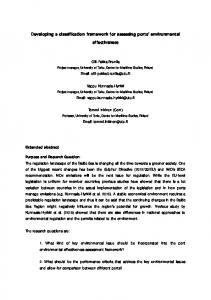
Figure 1. A hand radiograph (a) has been decomposed in regions on different scales. Scales are displayed for 0, 157, 1019, 1104, and 1130 iterations in (b), (c), (d), (e), and (f) respectively. Root
Root 8
Scale
2 1
1
2
3
Scale 3
3
2 1
4
5
4 6 8
7 1
4
9 10
6
5
6
Scale 2
7 Scale 1
8
9
10
Figure 2. The region hierarchy describes the inter-scale inclusion relation for each region between the scales. All edges in coarser scales have corresponding edges in finer scales (left). This causality leads to a tree structure (right), where each region is represented as a node (circles) with an attached feature vector (boxes). The edges represent a region’s inclusions. For a better overview, the neighbor adjacencies are not displayed in this figure.
feature space is performed without user interaction and is consequently independent from the underlying images and image domains as required. And finally, the classification framework provides the datamining cycle for learning new object descriptions efficiently.
3. HIERARCHICAL ANALYSIS OF IMAGE CONTENT Object identification is based on a generalized hierarchical image decomposition, which is fully automated executable at image acquisition time. In this work, a region growing algorithm was applied which starts with a complete watershed segmentation of the input image.24 From those segments, merge candidates are determined where the difference between homogeneity and contrast along the neighboring contour pixels is below a predetermined threshold. This procedure yields a multiscale representation of all visually plausible image regions (Fig. 1).
3.1. Data Structure The resulting data structure represents the topological adjacencies of regions by a region adjacency graph (RAG)26 as well as the inclusion relations induced by the multiscale approach. Therefore, it is called hierarchical attributed RAG (HARAG). In this graph, each image partition (i.e. region) is represented by a graph node. In the concept of the proposed image labeling method, it is assumed, that the hierarchical data structure contains every possible region that may be sought. From this point of view, object identification by a human examiner becomes the identification of appropriate image regions. This closes the semantic gap between low-level pixel information and high-level knowledge on image content. The formal representation of low-level information is an attribute vector. It is linked to a region node describes region properties such as size, roundness, texture, etc. (Fig. 2).
STRUCTURE
SHAPE
GREY VALUES
TEXTURE
Number of Sons Number of Neighbors Contour Length Absorption Iteration Creating Iteration Number of Holes Minimal Depth Maximal Depth Relative Size Relative Contour Length
Size Centroid X Centroid Y Relative Centroid X Relative Centroid Y Height of Ferret Box Width of Ferret Box Relative Height of Ferret Box Relative Width of Ferret Box Extent of Ferret Box Relative Height of Bounding Box Relative Width of Bounding Box Extent of Bounding Box Eccentricity of Bounding Box Orientation Principal Axis Radius Auxiliary Axis Radius Relative Principal Axis Radius Relative Auxiliary Axis Radius Eccentricity Radius of Fitting Circle Relative Radius of Fitting Circle Extent of Circle Form factor Roundness Compactness
Mean Gray value Relative Mean Gray value Variance Entropy
Contrast Variance of Coocurrence Matrix Differential Moment Entropy of Coocurrence Matrix Homogeneity of Coocurrence Matrix Correlation of Coocurrence Matrix Correlation1 of Coocurrence Matrix Correlation2 of Coocurrence Matrix
Figure 3. The currently available 48 attributes are categorized in four classes to represent different semantic views on image content. There are 10 sructural attributes (left) which basically serve as administrative data for the 38 descriptive features in the other classes.
3.2. Region Attributes Constant features are static information that is persistently stored within the HARAG file. It encloses the size of a region, the region pixels themselves as well as the adjacent and hierarchically included regions. Shape, grey value and texture features are computed from this basic information. To obtain normalized and consequently comparable values relative attributes are computed. They put the image dimensions in relation to the absolute values. The current set of attributes has been taken from literature and focuses on shape properties (Fig. 3). If necessary, the implementation is easily extensible by new attributes and attribute classes.
4. THE CLASSIFICATION FRAMEWORK Since the no free-lunch-theorem implies the necessity of experiments to determine a “good” classifier, the framework models the requirements of medical object extraction (Sec. 2) while providing a processing scheme that allows parameterization of all steps of the classification pipeline. The framework consists of four components and has been implemented as an open platform supporting standardized exchange of data between the modules as well as automatic report generation. For each step a set of state-of-the-art methods as applied by other approaches12–18 has been integrated to cover the basic principle of classifier design.11
4.1. Input Data and Evaluation The feature space that is generated by the hierarchical image decomposition provides the input data, where each vector is an item to be classified (Sec. 3). Variations and selections of training and test data are required independently from the distribution of the input data because of the following components. Besides manual partitioning, there are automated methods available.11 Since classification for object extraction corresponds to a retrieval task, the evaluation requires a ground truth with respect to the input data. The actual quality of a classification is measured with respect to the ground truth via precision, recall, and the F-measure, 20 which is defined as: 2 · recall · precision F-measure = (1) recall + precision
4.2. Classifier Selection Different paradigms of classifiers are characterized by their separation strategies. Model-free classification makes no assumption on the structure of classes. As model-free classifier the 1-nearest-neighbor (1-NN) is integrated with two distance measures: L2-norm (L2) and cosinus-norm (COS).11 Classifiers which minimize the empirical risc consider the distribution and likelihood for feature values within and between classes, and they yield optimal results yet for the price of overfitting. The Bayesian classifier with Gaussian Mixture Models (BGMM) is integrated for structural risc minimization, where the number of Gaussians is variable and the type of the covariance matrix can be selected. Overfitting is avoided by generalization which is provided by classifiers which minimize the structural risk.11 The support vector machine (SVM) integrates this paradigm. Here radial basis function and cross validation (CV) serve as parameters.21
4.3. Feature Selection for Dimension Reduction Feature selection is required to clean the feature space from redundant attributes and outliers which interfere without being discriminative. Hereby classifiers are not misguided by feature dimensions which do not contain discriminative information. Feature selection for dimensional reduction is performed by linear discriminant analysis (LDA), principal component analysis (PCA) and a greedy approach. The latter selects attributes which improve the classification result either by successively adding (up-greedy) or removing (down-greedy) the most or less improving attribute, respectively. Which feature selection yields best classifications depends on the input data and the classifier. This must be determined experimentally.
4.4. Application Scenario An application scenario corresponds to classifier training by random selection of a small set of training regions i.e. feature vectors from the available HARAGs. In real applications a region is selected by point-and-click training, where the user selects an image and browses to the scale in which respective region is represented. The positive class contains the selected regions while the negative class consists of all other vectors. Based on this two-classes, the classifier is trained and applied to the remaining set of computed HARAGs. It is assumed that the positive classified regions correspond to the user specified regions. In the simulation of the application scenario, a set of sample sets for a fixed size is selected randomly from the manually generated ground truth.
5. EXPERIMENTS Experiments always execute the full classification pipeline and vary a single component. To estimate the quality of a classification, its F-measure (Eqn. 1) is computed with respect to the ground truth.
5.1. Assessment of Experimental Results Since this is a novel approach to general biomedical object extraction there are no fully comparable results for the retrieval performance. Concepts based on non-medical data such as the Corel photo database typically use color information, and do not provide visually plausible multiscale information. 12–18 For medical applications there are either spezialized solutions for a single type of object, or there are approaches that represent global image content information. Solutions designed for specific tasks yield precisions betwen 0.9 and 0.98 on the sought objects,1, 2, 4 but they cannot be applied to other tasks. Their development is time-consuming and requires knowledge in computing and medical applications. Thus they are no general purpose retrieval tools with respect to the requirements formulated in Section 2. On the other hand current content-based image retrieval systems for medical applications which operate on global content description yield mean average precisions of maximal 0.4. This has been compared on a real-world medical reference database without textual annotations but with extensive a-priori training.28 Consequently results of pure object oriented retrieval without a-priori knowledge must be regarded qualitatively with respect to these limits. However the performance of all classifiers within each experiment is comparable without restriction.
5.2. Experimental Data and Ground Truth Reference application for the experiments is the extraction of metacarpal bones from hand radiographs. This is part of typical applications in computer aided radiology.3, 5, 6 A series of 105 radiographs is transformed into HARAGs of about 2,400 nodes each and for each of the corresponding regions a 38-dimensional feature vector is computed from the attributes of Figure 3, where the administrative attributes are ignored. 7 By using a graphical user interface, trained experts have selected the best fitting 372 regions for metacarpal bones from all HARAGs, which serve as a ground truth.27 From the total of 247,662 nodes in all HARAGs, the number of relevant regions is limited to those with a maximum deviation in the values of 0.8 and 1.2 of the minimum and maximum for each feature, respectively. This results in a database of 39,017 nodes.
5.3. Feature Selection for all Classifiers Experimental training data is a randomly selected subset of ten images corresponding to 43 from the 372 feature vectors. Aim of these experiments is understanding the structure of the feature space with respect to redundancy. The less dimension a classifier needs to obtain its best result the better is the separability of the classes. If there is a similar F-measure and dimensionality for different selection methods for a classifier, then the feature space would be considered as generally suitable for this classifier. Since the features mostly have a normal distribution the BGMM is expected to perform best. 5.3.1. Greedy Approach Feature selection via the up-greedy approach is verified for all three classifiers. 1-NN is applied with the L2 and COS distance measures. The SVM is applied using the Gaussian kernel and three partitions for cross validation since there is a maximum of five metacarpal bones per image, this ensures full partitions with one or more entries. The BGMM classifier is applied with a single distribution and variance pooling for the covariance matrix. The same approach is used for the down-greedy method. Aim of this experiment is to determine which classifier performs best with greedy selected features, and if there is a difference between the up- and down-greedy approach. The computation stops if there is no more improvement in the F-measure by selection or removing of a feature. 5.3.2. Dimension Reduction by PCA and LDA The dimension reduction by PCA and LDA is performed for all possible target dimensions between 1 and 38. It is assumed that increasing target dimension yields increasing F-measures.
5.4. Application Scenario for all Classifiers To simulate the real application of training and classification, sets of 5, 10, 20 and 40 regions are randomly drawn from the set of features that represent the metacarpal bones. This corresponds to point-and-click training with 1, 2, 4, 8 and 16 images respectively. For a realistic simulation of different users there are 20 different sets drawn for each number of training sets and the resulting average F-measure is considered. This is used to estimate the retrieval performance of each classifier in comparison to each other. Furthermore, the development of the classification quality with increasing training data is evaluated.
6. RESULTS 6.1. Feature Selection for all Classifiers The results of feature selection by the greedy approach (Sec. 5.3.1) are presented as two tables of classifier, number of resulting features, precision, recall and F-measure. While for the PCA and LDA the effect of dimensional reduction on the F-measure (Sec. 5.4 is presented as a function of the respective dimensions.
Classifier 1-NN, L2 1-NN, COS BGMM SVM
# Features 7 12 12 14
Recall 0,36 0,52 0,58 0,58
Precision 0,28 0,28 0,37 0,67
F-Measure 0,31 0,36 0,45 0,62
Table 1. F-measure, precision and recall for the up-greedy approach for all classifiers.
Classifier 1-NN, L2 1-NN, COS BGMM SVM
# Features 24 32 31 37
Recall 0,51 0,48 0,32 0,48
Precision 0,34 0,34 0,27 0,32
F-Measure 0,41 0,40 0,29 0,39
Table 2. F-measure, precision and recall for the down-greedy approach for all classifiers.
6.1.1. Greedy Approach For the up-greedy approach the SVM with the radial basis function kernel yields the best results (F-measure = 0.65) using CV with three partitions, while the 1-NN with the L2 distance performs weakest (F-measure = 0.4). Overall, the SVM performs best (Tab. 1). The number of features is hardly more than a quarter of all available features. For the down-greedy, the 1-NN yields best results independent of the norm, yet the SVM obtains nearly the same values. Here, the number of features ranges from nearly all for the SVM down to 24 for the 1-NN L2 (Tab. 2). 6.1.2. Dimension Reduction by PCA and LDA With the PCA the F-Measure increases nearly asymptotically with increasing dimension for all classifiers. Where the maximum value lies around 0.2. The SVM shows a slightly volatile development yet similar to the 1-NN with their steepest ascend at 5 dimensions while the results for the BGMM reach this point at 15 dimensions (Fig. 4). In contrast the LDA yields a completely indeterministic behavior along the target dimension for all classifiers. The SVM decreases from 0.3 to 0.15 while the BGMM varies between 0.05 and 0.205. the 1-NN L2 performs best between 0.205 and 0.31 (Fig. 4).
6.2. Application Scenario for all Classifiers The application of the sample sets (Sec. 5.4) yields an overall best performance for the SVM for all experiments. Yet for 20 bones the BGMM is slightly better obviously on behalf of the better recall value. Since the Fmeasures do not differ significantly, it must be considered that they represent the average value of 20 single queries with different training sets. A Wilcoxon test on these single results reveals there are no statistically significant differences up to 10 bones for 20 and 40 bones the differences between single sample results for each classifier vary significantly.
7. DISCUSSION 7.1. Feature Selection for all Classifiers Feature selection reveals the inhomogeneous structure of the feature space. Since the query results cover a wide range of values. It is interesting, that the simple greedy selection yields a better result for all classifiers, than the more complex correlated dimension reduction. However, this confirms the complex shape of the cluster for the metacarpal bones class with the applied features. Furthermore, the results cannot be generalized since there is no correlation between the results of different approaches. In one case the SVM is best but in the other, it performs worst. The 1-NN can be considered as the weakest classifier with the most constant results, while the BGMM also varies in classification quality.
LDA 0,35
0,3
0,3
0,25
0,25 F-Measure
F-Measure
PCA 0,35
0,2 0,15
0,2 0,15 0,1
0,1 BGMM 1-NN L2 SVM
0,05
BGMM 1-NN L2 SVM
0,05 0
0 0
5
10
15
20 25 Target Dimension
30
35
40
0
5
10
15 20 25 Target Dimension
30
35
40
Figure 4. F-measure for PCA (left) and LDA (right) reduced features for SVM, 1-NN L2 and BGMM.
# Training Objects 5 bones
10 bones
20 bones
40 bones
Classifier 1-NN, L2 BGMM (1) SVM 1-NN, L2 BGMM (1) SVM 1-NN, L2 BGMM (1) SVM 1-NN, L2 BGMM (1) SVM
Recall 0,25 0,28 0,26 0,27 0,50 0,24 0,29 0,30 0,35 0,32 0,60 0,38
Precision 0,26 0,26 0,29 0,28 0,22 0,44 0,29 0,30 0,43 0,33 0,28 0,52
F-Measure 0,25 0,25 0,25 0,28 0,30 0,28 0,29 0,30 0,37 0,33 0,38 0,42
Table 3. Results of classifiers with increasing number of bones.
7.2. Application Scenario for all Classifiers In the application scenario, the results improve as expected with an increasing training set, yet between 20 and 40 training vectors the result is only slightly improved. This indicates a sub-linear dependency of the classification quality from the amount of training data. The results further indicate that object extraction by classification on hierarchically decomposed images is possible. Though the results could be better, they can be compared to results that are currently obtainable from content-based image retrieval on global features. Here, state of the art systems yield a best mean average precision (MAP) of 0.48 only by combining textual and formal content description. 28 By pure content description, a best MAP of 0.40 is achieved.28 Using supervised machine learning to perform object extraction as a classification of hierarchically decomposed images is a novel approach. It enables the complete separation of generalized image segmentation and specialized but automated object extraction. Classical approaches to object retrieval via learning by example depend on semantical or statistical models for training of the retrieval algorithm, 14–18 which are integrated in the segmentation process itself. Consequently, the entire training and segmentation process has to be executed for each object and each image individually. Additionally, the user has to mark a sufficient number of relevant sample objects on a pixel level, which is cumbersome and more error-prone than its selection from a given partitioning. This makes those system unsuitable for medical applications where a-priori unknown objects are sought. Within our framework, the requirements of object retrieval systems for medical applications are considered comprehensively.
8. CONCLUSION It is possible to perform object extraction in medical images by classification on a high-level of semantic abstraction. In this case, point-and-click training of visually comprehensible regions is the only required user interaction for object retrieval from image series. However, the classification pipeline must be identified experimentally. The developed framework is an appropriate tool to verify the dependency of the classification result from the various degrees of freedom. In forthcoming experiments, the approach is to be validated on other retrieval tasks to understand the dependency of the classification pipeline from different feature distributions. It is also possible to integrate and evaluate other classifiers such as decision trees or Bayesian-belief network.
9. ACKNOWLEDGEMENT This work was performed within the image retrieval in medical applications (IRMA) project, which is supported by the German Research Foundation (Deutsche Forschungsgemeinschaft, DFG), grants Le 1108/4 and Le 1108/6. For further information visit http://irma-project.org.
REFERENCES 1. Madabhushi A, Feldman MD, Metaxas DN, Tomaszeweski J, Chute D; Automated detection of prostatic adenocarcinoma from high-resolution ex vivo MRI; Medical Imaging 2005; 24(12):1611–25. 2. Di Ruberto C, Dempster A, Kahn S, Jarra B; Analysis of infected blood cell images using morphological operators; Image and Vision Computing 2002; 20:133–146. 3. Manos G, Cairns AY, Ricketts IW, Sinclair D; Automatic segmentation of hand-wrist radiographs; Image and Vision Computing 1993; 11(2):100–111. 4. Metzler V, Lehmann T, Bienert H, Mottaghy K, Spitzer K; Scale–independent shape analysis for quantitative cytology using mathematical morphology; Computers in Biology and Medicine 2000; 30:135–151. 5. Vogelsang F, Kohnen M, Schneider H, Weiler F, Kilbinger MW, Wein BB, Guenther RW; Skeletal maturity determination from hand radiograph by model-based analysis; Procs. SPIE 2000; 3979: 294–305. 6. Pittman JR, Bross MH; Diagnosis and management of gout; American Family Physician 1999; 59(7):1799– 806. 7. Lehmann TM, G¨ uld MO, Thies C, Fischer B, Spitzer K, Keysers D, Ney H, Kohnen M, Schubert H, Wein BB; Content-based image retrieval in medical applications. Methods of Information in Medicine 2004; 43(4):354–61. 8. M¨ uller H, Michoux N, Bandon D, Geissbuhler A; A review of content-based image retrieval systems in medical applications. Clinical benefits and future directions; International Journal of Medical Informatics 2004; 73(1):1–23. 9. Metzler V, Thies C, Aach T; A novel object-oriented approach to image analysis and retrieval; Procs. 5th IEEE Southwest Symposium on Image Analysis and Interpretation 2002; 14–18. 10. Thies C, Metzler V, Aach T; Content-based image analysis: Object extraction by data-mining on hierchically decomposed medical images; Procs. SPIE 2003; 5032:579–589. 11. Duda RO, Hart PF, Stork DG; Pattern Classification; 2nd edition, Wiley Interscience, New York, 2001. 12. Djeraba C; Association and content-based retrieval; IEEE Transaction on Knowledge and Data Engineering 2003; 15(1):118–35. 13. Jiang W, Chan KL, Li M, Zhang H; Mapping low-level features to high-level semantic concepts in regionbased image retrieval; Procs. IEEE Computer Society Conference on Computer Vision and Pattern Recognition 2005; 244–9. 14. Carson C, Belongie S, Greenspan H, Malik J; Blobworld: Image segmentation using expectationmaximization and its application to image querying; Pattern Analysis and Machine Intelligence 2002; 24(8):1026–38. 15. Wang JZ; Integrated Region-Based Image Retrieval; Kluwer Academic Publishers, Dordrecht, 2001. 16. Xu Y, Duyuglu P, Saber E, Tekalp AM, Yarman-Vural FT; Object based image labeling through learning by example and multi-level segmentation; Pattern Recognition 2003; 36(6):1407–23.
17. Leibe B, Schiele B; Analyzing appearance and contour based methods for object categorization; Procs. Conference on Computer Vision and Pattern Recognition 2003; 409–15. 18. Leibe B, Schiele B; Interleaved object categorization and segmentation; Procs. British Machine, Vision Conference 2003; 759–68. 19. Fukanaga K; Introduction to Statistical Pattern Recognition; 2nd edition, Academic Press, New York, 1990. 20. van Rijsbergen CJ; Information Retrieval; 2nd edition, Butterworths, London, 1979. 21. M¨ uller KR, Mika S, R¨atsch G, Tsuda K, Sch¨olkopf B; An introduction to kernel based learning algorithms; IEEE Transactions On Neural Networks 2001; 12(2):181–202. 22. Dempster AP, Laird NM, Rubin DB; Maximum likelihood from incomplete data via the em algorithm; Journal of Royal Statistical Society 1977; B(39):1–38. 23. Witten IH, Eibe F; Data-mining: Practical Machine Learning Tools and Techniques with Java Implementations; Morgan Kaufman Publishers, San Francisco, 2000. 24. Lehmann TM, Beier D, Thies C, Seidl T; Segmentation of medical images combining local, regional, global, and hierarchical distances into a bottom-up region merging scheme; Procs. SPIE 2005; 5747:546–555. 25. Thies C, Malik A, Keysers D, Kohnen M, Fischer B, Lehmann TM; Hierarchical feature clustering for content-based retrieval in medical image databases; Procs. SPIE 2003; 5032(1):598–608. 26. Sonka M, Hlavac V, Boyle R; Image Processing, Analysis and Machine Vision. Chapman & Hall, London, 1993. 27. Thies C, Ostwald T, Fischer B, Lehmann TM; Object-based modeling, identification and labeling of medical images for content-based retrieval by querying on intervals of attribute values; Procs. SPIE 2005; 5748:382– 391. 28. Clough P, M¨ uller H, Sanderson M; The CLEF 2004 Cross-Language Image Retrieval Track; LNCS 3491:597–613.