edition of the DARPA Grand Challenge [1]. The US Defense. Advanced Research Programs Administration (DARPA) cre- ated this robotic vehicle competition as ...
A Decision Network Based Frame-work for Visual Off-Road Path Detection Problem Alberto Broggi, Claudio Caraffi, Stefano Cattani, Rean Isabella Fedriga VisLab-Dipartimento di Ingegneria dell’Informazione, Universit`a di Parma, Parma I-43100, Italy {broggi,caraffi,cattani,fedriga}@ce.unipr.it
Abstract— This paper describes a Decision Network based frame-work used for path-detection algorithm development in autonomous vehicle applications. Lane marker detection algorithms do not work in off-road environments. Off-road trails have too much complexity, with widely varying textures and many differing natural boundaries. The authors have developed a general approach. Images are segmented into regions, based on the homogeneity of some pixel properties and the resulting regions are classified as road or not-road by a Decision Network Process. Combinations of contiguous clusters form the path surface, allowing any arbitrary path to be represented.
I. INTRODUCTION On October 8th, 2005 twenty-three vehicles and no drivers gathered in the Mojave desert to compete in the second edition of the DARPA Grand Challenge [1]. The US Defense Advanced Research Programs Administration (DARPA) created this robotic vehicle competition as an open challenge intended to energize the engineering community to tackle the major issues confronting autonomous vehicle development. For the timed competition, DARPA designed a 132-mile offroad desert course that each vehicle had to negotiate. The course was defined by an ordered list of geographic waypoints, a maximum speed for each waypoint and boundaries that could not be crossed. Vehicles had to operate with full autonomy as they maneuvered around obstacles lining the desert course. This paper presents an artificial vision algorithm developed as a part of the TerraMaxTM vehicle. Oshkosh Truck Corporation, Rockwell Collins and the University of Parma partnered together to form Team TerraMaxTM [2]. The Team TerraMaxTM robotic vehicle (Fig. 1) is a US Marine Medium Tactical Vehicle Replacement (MTVR) truck which was fitted with electronic actuators for steering, brake, throttle, and transmission control. A computer network was installed to host the software applications necessary for autonomous navigation. The applications consisted of vehicle control, path planning, LIDAR obstacle detection, and artificial vision obstacle detection and path following. The Artificial Vision and Intelligent Systems Lab (VisLab) of the University of Parma developed the artificial vision systems that sensed the environment. Three color cameras captured video images; a single computer processed the data. Obstacle detection used stereo vision and a v-disparity This work was supported by Oshkosh Truck Corporation
Fig. 1.
The TerraMaxTM vehicle
approach. Path detection used monocular images and the approach discussed in this paper. II. PATH DETECTION AS A DECISION PROBLEM Path detection on structured environments has been already successfully faced by the authors [3] and others [4], using monochromatic monocular images and assuming the existence of lane markers. Unfortunately on unstructured and unknown environments is not possible to rely on any a priori knowledge about road structure. To overcome this lack of information many different approaches have been proposed: learning the road properties by neural networks [5], selecting the actual road-borders within the set of all possible curves on the image by evolutionary techniques [6], and growing regions believed to belong the road, on the basis of some a priori assumptions or simplifications. All these methods look for a single homogeneous road surface in front of the vehicle, searching based on brightness, color, texture, etc. The hypothesis of uniform homogeneity becomes a huge limitation as it bounds the set of detectable roads to the case of medium/well structured environments. The proposed method differs from the above methods, overcoming their limitations by generalizing the problem. Roads can have heterogeneous surfaces. To find these potentially heterogeneous surfaces, the algorithm looks to build them up from a variable number of smaller homogeneous terrain portions. The homogeneous portion of terrain can represent any kind of natural or artificial environment elements,
such as gravel or paved roads but also grass, water paddle, oil stains, drivable rocks, lane markers, shadows, etc, and they do not need to be previously learned and recorded in a database [7]. Consequently it is possible to summarize the path detection algorithm as a two-step process: • divide the image in homogeneous regions made of connected pixels. • decide which combination of the obtained regions could represent the road surface with the highest probability. The first step is called clustering, or image segmentation. Clustering in computer vision has been being studied with success, especially for medical applications, using both evolutionary [8] and traditional [9] [10] approaches. However the real-time constraints of the Grand Challenge contest led to the adoption of a simple but fast and easily tunable clustering algorithm, explained in Section III, as a good trade-off between performance and computational requirements. The second step falls in the class of decision problems. Born to help decision processes in medical, transportation, political or environmental fields, decision theory [11] is now widely used by Artificial Intelligence researchers as a useful frame-work into which they can map a variety of classical problems. Decision Networks [12] extend Bayesian networks, adding actions and utilities to provide a general methodology for rational decision making. Section IV will describe how Decision Network fits the problem of decide about the set of clusters that belong to the road surface. The decision process tries to minimize the risk of wrong classifications taking into account the current vehicle state given by speed, steering angle, steering angle acceleration. This approach has the advantage of explicitly shifting the path detection to a high level problem, allowing a wider range of situations to be handled in a more sensible way. For example there is no need to remove vehicle shadows at a medium/lower level, on the basis of brightness considerations. In fact since vehicle shadows belong to the terrain surface, its corresponding cluster will be treated just as any other region: like a potential part of the road. III. CLUSTERING Several image segmentation algorithms can be found in literature. The most common approach is to join close pixels to obtain a large region composed by similar entities. In approach described in this section, images are decomposed in d · d pixels cells and a comparison is made among them. The use of cells instead of pixels allows a comparison using both the average color value and the information about the texture, like variance. A. Pseudo Distance Function To measure the similarity of cells we defined a pseudo distance function, that combines distances from cell to cell, from cluster to cluster, and from cell to cluster. Before introducing the distance function it is necessary to define the following entities:
A set C of ci,j , where ci,j =< xk1 , xk2 , ...xkn >= ck ∈ ∈ < is the properties vector of the k − th cluster of cells 1 . The partial comparison functions are defined as follows: • the cell to cell only comparison function is: n X c2c(ck , cl ) = Di−c2c (xki , xli ) · αi , ∀ck , cl ∈ C (1) •
i=0 •
the cluster to cluster only comparison function is: n X v2v(vk , vl ) = Di−v2v (yki , yli ) · αi , ∀vk , vl ∈ V i=0
•
(2) the cell to cluster only comparison function is: n X c2v(ck , vl ) = Di−c2v (xki , yli )·αi , ∀ck ∈ C and vl ∈ V i=0
(3) where αi ∈ . Clusters properties vectors vk are made of the corresponding cells’ average HLS values: < (H k , σHk ) , (Lk , σLk ) , (S k , σSk ) > = < (µk1 , σk1 ) , (µk2 , σk2 ) , (µk3 , σk3 ) > = < yk1 , yk2 , yk3 >. Cell to cell (1) partial comparison functions take the following form:
Di−c2c (xki , xli ) =
[j]
[j]
j=1 |xki − xli | p σx2ki + σx2li
(12)
Cluster to cluster (2) partial comparison functions use cluster averages and variances: |µki − µli | Di−v2v (yki , yli ) = p 2 2 σki + σli
(13)
Cluster to vector (3) partial comparison functions also use averages and variances: |xki − µli | Di−c2v (cki , yli ) = q 2 σx2ki + σli
(14)
All the above functions are greater or equal than zero. Moreover, (12) and (13) are commutative, and to (13) also applies: Di−c2c (a, b) = 0 ⇐⇒ (a = b). B. Clusters properties The clusters properties yj used to compute the probability functions pj in (11) are:
Name y1 y2 y3 y4 y5
Property Average variance of cells’ HLS values. Number of cells (%). Percentage of cells contained in the freespace. Position and form factors 1. Position and form factors 2.
Each property value is normalized to [0, 1] ∈