A Global Path Planning System using Local Navigation Strategies Alex Tay*1, Javier Ibanez Guzman2, Shen Jian2, Lee Keok Kee1, Chan Chun Wah3 1
School of Computer Engineering, Nanyang Technological University, Singapore {aslptay, askklee}@ntu.edu.sg 2 Singapore Institute of Manufacturing Technology, Singapore {javierg, jshen}@SIMTech.a-star.edu.sg 3 Defence Science Technology Agency, Singapore
[email protected]
Abstract In an obstacle filled environment, path planning solutions that use accurate Global Positioning System (GPS) coordinates of obstacles need to reconsider the inaccuracies of positioning when the differential GPS is not available. Typical GPS positioning systems operating without the differential component, are able to provide a default Central Error Probability (CEP) of only 10m. It is not always possible to install additional differential beacons in unexplored territory to reduce that error. This paper presents a path-planning algorithm and a novel global navigation strategy for autonomous unmanned ground vehicles (AUGV) in an unstructured terrain. An introduction of the AUGV architecture provides the basis for which the novel strategy is used to navigate through a global environment. It is able to chart a path along roadways and off-road terrain. Keywords – Autonomous Unmanned Ground Vehicle (AUGV), Global Positioning System (GPS), Path Planning, Distance Transform, Voronoi Diagram.
1.
Introduction
Path planning in the outdoor environment has been a widely studied field [1,2,3]. Many studies have produced efficient path planning strategies [4,5,6]. However, the issues arising due to limited GPS resolution have often been overlooked. In situations where the GPS has to operate alone, the vehicle’s relative position to obstacles may change due to unstable GPS readings. This makes it difficult for the vehicle to avoid obstacles and navigate across the global environment at the same time. This paper presents a path planning algorithm and strategy for autonomous vehicles traversing through an obstacle field, characterized by convex obstacle formations. It addresses the problem of navigating through an obstacle field using localized maps generated with the aid of the vehicle’s visual system and yet bearing the ability to navigate globally. A brief description of the available sensors is provided as a means to understand
the algorithm. Figure 1 shows the picture of the experimental vehicle used in this investigation.
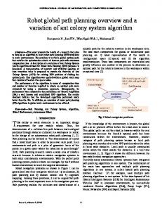
1.1. The Global Positioning System (GPS) The GPS system used in our experiments provided information at a refresh rate of 10 Hz with CEP of 10m, which translates to an accuracy of ± 10m at 100ms intervals. The stand-alone GPS often registers inconsistencies in coordinate reporting when certain satellites are suddenly lost from the GPS reception [3]. This may happen when some satellites suddenly go into receiver shadow regions, and therefore, it becomes impossible to receive geolocational information from them. Figure 2 shows the results of an experiment in which the vehicle was autonomously driven along a cyclic route using the GPS system. The actual route travelled during the recording, was a regular ellipsoid. The positional variations of ±5m recorded in the experiment (as shown by the protrusions into and out of the ellipsoid) highlight the potential difficulty for path planners that assume correct relative GPS positions between the vehicle and the obstacles. Collision is likely to occur if these uncertain conditions were posed on a 3 m wide vehicle travelling on a 7 m wide road lined with obstacles.
Figure 1. The experimental platform
External Input
Navigation Module
352930 352920
UTM Northing (m)
352910
Positioning Module
Elevation Analysis
Centroid Finding Module
Planner
Terrain Sensor Fusion
352900 352890
Local Map
Module Output Heading and Speed
Global Map
Figure 3. The Navigation Module Architecture
352880
2.1. Assumptions of the Terrain 352870
Several assumptions and operating conditions are defined prior to designing the algorithm. These conditions of the navigator include the following:
352860 352850 149300
149310
149320
149330
UTM Easting (m)
1. All obstacles within the navigation space are convex in nature and do not form cul-de-sacs. Any consolidation of obstacles within the navigational space is also assumed to be convex in nature.
Figure 2. Results showing multi-path distortions
1.2. The Navigation Module Interface The navigation unit, a sub-system in the AUGV system, was itself interfaced to 3 other input subsystems and a single output subsystem. The output subsystem receives the desired heading and the desired speed information from the navigation module and transmits this information to the vehicle control system. The 3 input subsystems include the GPS module, the laser sensor module and the centroid finding module. Figure 3 shows the architecture of the planner with respect to its neighboring subsystems.
2.
The Modified DT Algorithm
After comparing several algorithms in path planning, the Distance Transform [DT] algorithm [3,4,5] was selected because it required the least number of compare operations for this application. The DT algorithm was subsequently used as a basis of this work and built upon to produce a more complex and robust algorithm for the proposed architecture. The DT algorithm was modified to create a Modified Distance Transform Algorithm (MDT) that used preferred route conditions and longitudinal C-Space growth for obstacle avoidance at higher speeds. The paragraphs that follow describe the MDT Algorithm.
2. No a priori information regarding the position of obstacles is available in the provided global map. The global map consists only of GPS target points which the vehicle is expected to pass through or reach. These GPS target points are assumed to be reachable and free of obstacles. 3. An m x n grid map is obtained from the laser vision system observing an actual frontage of 15m x 15m square in front of the vehicle. The visual space of 15m x 15m is laterally symmetrical to the mid-lateral axis of the vehicle, such that 7.5m of the space is on the left and 7.5m of the space is on the right of the vehicle. In front of the vehicle is a 3m deep blind spot, after which begins the 15m viewing depth. The view depth from the lasers is therefore 18 m in front of the vehicle. Figure 4 illustrates the laser field of view. Sensor fusion techniques were essential to obtain the local map.
2.2. Algorithm Description The algorithm begins with an initialization of the 2D m x n grid map into cells Cij [where (i,j) is the cell found on the coordinate (m,n)]with a cell traversal cost of Tij and a cell value of Vij initialized to a very large number k. Cend and Cstart are special instances of Cij, Cend denoting the end point cell and Cstart denoting the start point cell. Obstacles are denoted by Bij. Upon execution of the algorithm, Vij stores the representative
This allows the executing algorithm to bias towards using the available road. If the cell is not a centroid, then Tij will retain the default initial setting of 3.
15m x 15m space converted to
The obstacle map obtained from the laser visual system provides information of non-traversable areas that are overlaid onto the map with high Tij values. In order to work with vehicular widths, the concept of obstacle Configuration Space (C Space) is used and grown onto the overlaid map. Positions adjacent to the obstacles are given similar high weights. This process renders the C Space around the obstacle non-traversable.
75 x 75 Grid Occupancy Map
3m Blind Dead Space Vehicle C Figure 4. Occupancy map of 75 x 75
distance between the Cij and Cend. The variable Tij is used as a function to calculate the cost of a planned path. Tij contains a numeric value that grades the difficulty of passing through the particular cell Cij. In the case of the experiments conducted Tij used the values shown in Table 1. Path Description Road Cross Country (ie. off-road) Trench Obstacle
Tij 1 3 5 9999
Table 1. Settings for Tij under various conditions
The lower values indicate easier traversing conditions. Conditions that lead to lower values for Tij are roads and previously cleared pathways. In the implementation, the m x n grid map is the 75 x 75 Grid Map obtained from a visual transformation of the pair of lasers mounted at the front of the vehicle. The Vij values of all cells were initialized to a very large number k that fulfills the condition
k>
After the recursive stage is complete, the algorithm proceeds with the lowest potential search, beginning from Cstart. The algorithm determines the next cell amongst the current cell’s neighbors that possesses the lowest VALUE. The lowest valued cell will be chosen as the next cell and the algorithm continues until the end point is reached. The complexity of this portion of the algorithm is less than O(n) as it would only need to search the points from the start position to the end position bearing lowest Vij values. 1
i=m, j =n
∑T
i =0, j =0
The algorithm begins at Cend. At each adjacent cell to Cend, the algorithm performs the small computation process of adding Tij of the lowest valued neighbor to the Vij of the current cell and placing the result in the current Vij. Each cell’s computation requires a search of its 8 adjacent neighbors and each cell is visited only once. This constitutes to a computational complexity of this part of the algorithm is O(n), where n is the number of cells within the grid map. The process will continue until all cells have been processed, or the start point has been reached. If Tij was based on a constant value of 1, recursion beginning at Part 6 can be omitted. However, due to the cost structure of the preferred routes and off-road routes, path exceptions may occur. This exception is explained in Section 2.3. The recursive algorithm is essential for the correct formation of the cost map. It is therefore necessary to re-evaluate the COST Vij of each cell.
ij
(1)
In the implementation, the value of k was set at 999999. The road centroid information was obtained from a colour segmentation module that derives the estimated road centre. If roads exist in the captured scene, the road centroids are used as preferential paths. The cell marked as a road centroid will carry a Tij value of 1.
2 3 4
Initialize the entire m x n grid map COST Tij = 3 and Vij = large number. Where ij is the indexed cell in question. Overwrite all road centroid positions found on m x n grid map with Tij = 1. (Centroid information is obtained from the Road Detection Camera). Overwrite all obstacle positions, Bij and obstacle C Space with Tij = 9999. Given the start Cstart and end points Cend in the m x n grid map, Begin at Cend, and set Vij to 0. Place 8 Cij neighbors into a FIFO Stack. Mark each CELL placed in Stack as PROCESSED
5
6
7
while stack is not empty, { Pop next Cij from Stack. If Tij != 9999, then determine lowest neighboring value and add Tij to obtain current CELL Vij. Determine if neighbor CELLS are processed. { If PROCESSED, skip CELL, Otherwise place CELL in stack and mark as PROCESSED. } } For (Every other CELL within GRID) { if CELL is obstacle skip. Else RECURSIVE_REDUCE_COST: { Determine value of lowest value neighbor. If current CELL Vij!= lowest Vij value neighbor + Tij, then { Vij = lowest value Vij + Tij. For all neighbors RECURSIVE_REDUCE_COST } } To track shortest path, Locate START point Cstart. Locate next neighboring CELL with lowest Vij. Continue locate lower Vij for next CELL until END Cend is reached or lowest VALUE is k. If k is reached, it implies no solution to be found.
2.3. The MDT Recursive Re-Evaluation This section illustrates how the DT algorithm suffices only in a situation where Tij is constant. If a multi level COST structure for Tij is designed, the need for recursive evaluation is necessary. Figure 5 shows the grown region using the DT algorithm with a constant Tij. Note that as the algorithm wraps its incremental expansion around the obstacle delineated by ∞, the Vij values will eventually meet on the other side of the obstacle. Figure 6 shows the grown region with the same algorithm, but the values for Tij are no longer constant. The lower portion of the grid map is attributed as cross-country values of Tij = 3 and the upper portion is attributed as Tij = 1. Note that as the algorithm expands around the obstacles, there is inconsistency between the upper half and lower half values for Vij, such that the point of convergence, located beyond the obstacle growth, does not represent a contiguous change between neighboring Vij. The highlighted regions bearing values of 27, 30 and 36 indicate the fault line in the DT expansion. The Modified DT includes a recursive component that removes this imbalance inherent in maps with varying Tij values. If recursion were performed as recommended in the MDT, the Grid map will be restructured into the representation shown in Figure 7.
2.4. Experimental Results of the MDT Algorithm The algorithm presented in Section 2.2 was the basis for the resultant simulation shown in this section. Figure 8 illustrates possible problems that obstacles
Figure 5. Results of the DT expansion with constant Tij (The higher order portion of tenths is omitted for purpose of illustration.)
Figure 6. Results of DT expansion with varying Tij
12 12 12 12 12 12 12 15 15 18 21
9 9 9 9 9 9 12 12 15
8 8 8 8 8 8 9 12 15 18 21 21
7 7 7 7 7 8 9 12 15 18 21
6 6 6 6 7 8 9 12 15 18 21
5 5 5 6 7 8 9 12 15 18 21
4 4 ∞ ∞ 7 ∞ 11 12 15 18 21
3 3 ∞ ∞ ∞ ∞ ∞ ∞ 15 18 21
2 2 ∞ ∞ ∞ ∞ ∞ ∞ ∞ 18 21
2 1 1 3 6 9 12 15 18 21 21
2 2 1 1 1 3 3 6 6 9 9 12 12 15 15 18 18 21 21 24 24
Figure 7. Balanced MDT due to recursive reduction
cause to vehicles requiring width clearance. Even though a road may exist, the presence of an obstacle on the side may render the path non-passable. The algorithm decides to navigate a segment on off-road terrain before utilizing the road again. Figure 9 shows a complex scene in which trenches were also considered. The purpose of the simulation was to ascertain the principles of the algorithm. Changes were made to the Ti structure to include Ti = 15 for trenches, the trenches. By using algorithm’s flexibility was improved to address tracked vehicles, such as work site excavators, to cross small trenches. These trench crossing tasks were non-trivial problems as it would be necessary for the vehicle to cross perpendicular to the trench. It turns out that the algorithm is able to locate the best positions for traversals and the solutions are inherently perpendicular to the trench axis. Figure 9 is a complex combination of obstacles, preferred routes and trenches, which the MDT algorithm was used to overcome. End Pt
Trenches are difficult entities because they bear properties of both an obstacle and a traversable cell. If the trench is too wide, the cells within cannot be traversed, making it an obstacle. If it is less than a certain width such that tracked vehicles can cross it, the cells then become traversable. The roaded path illustrated in the diagram indicates the preferred path. This information is obtained from the road centroid module. An obstacle was placed on the side of the road. This obstacle was meant to pose as an obstruction to the width of the vehicle. The path plan eventually follows the road half the way and then switches to perform a cross-country maneuver. As it performs a cross-country mode, the planner also takes the most economical path across the trench. The total time taken for the algorithm to compute one cycle is approximately 100 ms on a 700 MHz single processor. Unlike systems that require the user to switch between road following and crosscountry operation modes, the MDT algorithm described adaptively uses the most appropriate method.
2.5. Global and Local Planning Capabilities When the typical GPS reports with ± 10m CEP, deterministic navigation using mere GPS data would be unreliable. Planning around obstacles would become dangerous and the autonomous vehicle may collide with the obstacles due to the degree of uncertainty in the GPS information. Given that the local visual view is accurate to the degree of the vehicle sensors (± 0.2m), it is possible for the vehicle to avoid obstacles using the information obtained from the m x n visual map. The strategy used
End Pt Obstacle
Obstacle Start Pt
Start Pt (i)
(ii)
Figure 8. (i) Shows a roaded path with side obstacles. (ii) Shows the path planned after considering the width of the vehicle.
Figure 9. Complex environment test with trenches.
was to reliably link the m x n maneuver space with the global space. The successful bridge of these two spatial quantities was achieved using the Voronoi diagram and the result was resilient to GPS errors. The transformation of the global target into the local visual space is done by locating the point within the local view, that is nearest the final global target.
In this way, the test vehicle will have a target point within the local view, which it will lead the vehicle towards the global goal. Navigating around obstacles is achieved using a localized view obtained from the m x n map. The navigation module partitions the problem into two portions [4].
3.
Conclusions
Unlike most navigational strategies that use a voting steering method, the method presented here utilizes a direct calculation based on the obstacles within the local view and a global target. A Modified Distance Transform [MDT] algorithm is presented. Some of the advantages of using this algorithm are listed. 1) Basic algorithm is simple, inexpensive and robust with a complexity of O(n). 2) Ability to compute paths within 50 ms for a 75 x 75 grid space. 3) Ability to compute paths with obstacles and semi obstacles such as trenches 4) Ability to consider preferred paths formed by roads and desirable traversable routes. 5) Ability to compute paths along roadways or on off-road terrain without having to switch between the two. With the improvements in the MDT algorithm, it is shown that the calculations required are not complex and computationally inexpensive. As a result, the algorithm was able to perform frame-wise calculations of 10 Hz. The MDT is an effective algorithm in its own right. Designing the global path planner around this algorithm is key to the success of the strategy as the speed required to close the loop between image frames becomes possible. Throughout the actual execution of the path planner on an AUGV, it was noted the path planner was very stable and it was able to perform path planning for a
circular route of about 1km in length. Although the GPS sometimes provided random errors of ±5m, these did not affect the path planner’s ability to navigate the vehicle to close proximity of the global target. Errors would occur only when the vehicle was close to the global target point.
4.
Acknowledgements
The research was sponsored by Defence Science Technology Agency (DSTA) and A*STAR SIMTech.
5.
References
[1] Alonzo Kelly and Anthony Stentz, An Analysis of Requirements for Rough Terrain, Autonomous Mobility, Robotics Institute, Carnegie Mellon University, Pittsburgh, PA 15213. (Internal Publication) [2] Chin Yew Tuck, Wang Han, Tay Leng Phuan, Wang Hui, William Soh, Vision Guided AGV Using Distance Transform, Proceedings of the 32nd International Symposium on Robotics, April 2001. [3] D. Bouvet and G. Garcia. Civil engineering articulated vehicle localization: Solutions to deal with GPS masking phases, Proceedings of 2000 IEEE International Conference on Robotics and Automation, San Francisco, CA, Apr 2000. [4] Tay Leng Phuan, Javier Ibanez Guzman, Shen Jian, Chan Chun Wah, Autonomous Vehicle Navigation Strategies – Localized Navigation with a Global Objective, ICITA, Dec 2002. [5] R.A. Jarvis, Distance Transform Based Collision Free Path Planning for Robot, Advanced Mobile Robots, World Scientific Publishing, pp 3 – 31, 1994 [6] T. Aono, K. Fujii, S. Hatsumoto and T. Kamiya. Positioning of Vehicle on undulating ground using GPS and dead reckoning, Proceedings of the 1998 IEEE International Conference on Robotics and Automation, pp 3443-3448, Leuven, Belgium, May 1998.