A Network Flow Algorithm for Binary Image Reconstruction from Few ...

A Network Flow Algorithm for Binary Image Reconstruction from Few Projections Kees Joost Batenburg1,2 1

Leiden University, P.O. Box 9512, 2300 RA Leiden, The Netherlands 2 CWI, P.O. Box 94079, 1090 GB Amsterdam, The Netherlands

Abstract. Tomography deals with the reconstruction of images from their projections. In this paper we focus on tomographic reconstruction of binary images (i.e., black-and-white) that do not have an intrinsic lattice structure from a small number of projections. We describe how the reconstruction problem from only two projections can be formulated as a network flow problem in a graph, which can be solved efficiently. When only two projections are used, the reconstruction problem is severely underdetermined and many solutions may exist. To find a reconstruction that resembles the original image, more projections must be used. We propose an iterative algorithm to solve the reconstruction problem from more than two projections. In every iteration a network flow problem is solved, corresponding to two of the available projections. Different pairs of projection angles are used for consecutive iterations. Our algorithm is capable of computing high quality reconstructions from very few projections. We evaluate its performance on simulated projection data and compare it to other reconstruction algorithms.

1

Introduction

Tomography deals with the reconstruction of images from a number of their projections [1, 2]. In many applications, such as the reconstruction of medical CT images, a large number of different pixel values may occur in the reconstruction. Typically, the number of projections that is required to obtain sufficiently accurate reconstructions is large in such cases (more than a hundred). For certain applications, however, it is known in advance that only a few possible gray values may occur. Many objects scanned in industry for nondestructive testing or reverse engineering purposes are made of one homogeneous material, resulting in two possible gray values: the material and the surrounding air. Another example is medical digital subtraction angiography, where one obtains projections of the distribution of a contrast in the vascular system. The field of discrete tomography deals with the reconstruction of images from a small number of projections, when the set of pixel values is known to have only a few discrete values [3]. By using this prior information about the set of possible values, it may be possible to dramatically reduce the amount of projection data that is required to obtain accurate reconstructions. A. Kuba, L.G. Ny´ ul, and K. Pal´ agyi (Eds.): DGCI 2006, LNCS 4245, pp. 86–97, 2006. c Springer-Verlag Berlin Heidelberg 2006 

A Network Flow Algorithm for Binary Image Reconstruction

87

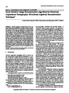
In [4] the author proposed an algorithm for reconstructing binary images that are defined on a lattice, using smoothness assumptions. This algorithm exploits the fact that the reconstruction problem for only two projections can be solved in polynomial time. The proposed reconstruction procedure is iterative: in each iteration a new reconstruction is computed using only two projections and the reconstruction from the previous iteration. The new reconstruction simultaneously resembles the image from the previous iteration and adheres to the two selected projections. In this paper we describe a new iterative algorithm for reconstructing binary images that do not have an intrinsic lattice structure (i.e., subsets of the plane), which is based on ideas similar to those used in [4]. To solve the twoprojection subproblems efficiently, a different pixel grid has to be used in each iteration, corresponding to the selected pair of projections. The reconstruction problem can then be solved as a special case of the minimum cost network flow problem in graphs, for which efficient polynomial time algorithms are available [5]. In [6] a more general version of our algorithm is described and more details are provided on the algorithmic steps. We refer the reader to that paper for further details. We restrict ourselves to parallel beam tomography. Let D = {θ1 , . . . , θd } be a set of disjoint real numbers in the interval [0, π), the projection angles. Let n be a positive integer. For i = 0, . . . , n, put ti = −n/2 + i. Let θ ∈ [0, π). For t, t ∈ R, t < t , define the strip Sθ (t, t ) as    2 x cos θ + y sin θ ≥ t and Sθ (t, t ) = (x, y) ∈ R : . x cos θ + y sin θ ≤ t

 

¾ 

 ½

(a)

(b)

Fig. 1. (a) Left: Schematic view of the parallel beam geometry which contains the lines L1 : x cos θ+y sin θ = 0 and L2 : x cos θ+y sin θ = t. (b) Right: A two-projection image.

88

K.J. Batenburg

Figure 1a shows the geometric meaning of the last definition. Define the imaging area I as d  I= Sθk (t0 , tn ). k=1

We will now define the basic reconstruction problem of reconstructing a binary image (i.e., black-and-white) from few projections. We consider the unknown image as a mapping f : I → {0, 1}. Problem 1. Let p1 = (p11 . . . p1n )T , . . . , pd = (pd1 . . . pdn )T ∈ Rn be vectors of nonnegative real numbers (the measured strip projections for projection angles θ1 , . . . , θd ∈ D respectively). Construct a function f : I → {0, 1} such that  f (x, y) dy dx

=

pki

for i = 1, . . . , n, k = 1, . . . , d.

Sθk (ti−1 ,ti )

 We call an integral of the form Sθ (ti−1 ,ti ) f (x, y) dy dx a strip projection. k In the next section we deal with the reconstruction problem from only two projections, which is severely underdetermined. In Section 3 we describe our iterative algorithm for reconstruction from more than two projections. Experimental results of the algorithm from Section 3 are presented in Section 4.

2

Reconstruction from Two Projections

This section deals with the reconstruction problem from only two projections, for angles θ¯1 and θ¯2 . To represent a mapping f : I → {0, 1} in a computer we have to resort to an approximate representation. An image f is represented as a 2D array of pixels. Every measured strip projection then gives rise to a linear equation on the pixel values of f . The resulting system of linear equations can be solved by methods from linear algebra, but in this way one cannot guarantee that a binary solution is found. We now introduce a particular grid, the twoprojection grid, for which a binary solution of the reconstruction problem can be found efficiently. The rows and columns of this grid correspond to the strips for the two projections angles θ¯1 and θ¯2 . Define grid cell Cij (1 ≤ i, j ≤ n) as Cij = Sθ¯1 (ti−1 , ti ) ∩ Sθ¯2 (tj−1 , tj ). A two-projection image is a mapping {1, . . . , n} × {1, . . . , n} → {0, 1} which assigns a binary value to each grid cell of a two-projection grid. Figure 1b shows an example of a two-projection image. It is often convenient to consider a two-projection image X as a matrix (xij ), where xij denotes X((i, j)) (the pixel value of cell Cij ). The strip projections of X for the projection angles θ¯1 and θ¯2 can be computed directly by summation of all entries in each row of X, or column respectively, and multiplying the result by the cell area a. For k = 1, 2, define Pk (X) ∈ Rn as the vector of strip projections

A Network Flow Algorithm for Binary Image Reconstruction

89

 of X for angle θ¯k . Define the one-count of X by S(X) = 1≤i,j≤n xij . We denote the area of a single grid cell by a. Note that all grid cells have the same shape and size. We will now define a reconstruction problem for two-projection images. As the projection data may contain noise or other errors, we don’t require that the image adheres perfectly to the measured projection data. In the next section, where we consider reconstruction from more than two projections, we require a generalization of the reconstruction problem which incorporates prior knowledge. We state this general reconstruction problem here. Problem 2. Let θ¯1 , θ¯2 ∈ [0, π) be two disjoint projection angles. Let p1 , p2 ∈ Rn be two vectors of nonnegative real numbers (the measured projection data). Let W = (wij ) ∈ Rn×n , T¯ ∈ N>0 and α ∈ R. Construct a matrix X ∈ {0, 1}n×n such that S(X) = T¯ and  awij xij α(|P1 (X) − p1 |1 + |P2 (X) − p2 |1 ) − 1≤i,j≤n

is minimal. In any instance of Problem 2, the one-count S(X) is considered to be fixed at T¯. A good value for T¯ can be computed from the measured projection data by taking T¯ = (|p1 |1 + |p2 |1 )/2a. Putting α = 1 and wij = 0 for 1 ≤ i, j ≤ n, yields the basic reconstruction problem (without the use of prior knowledge). The matrix W is called the weight map. The weight map is used extensively in the algorithm for reconstructing a binary image from more than two projections that we describe in the next section. It is used to express a preference for each pixel to obtain a value of either 0 or 1 in the reconstruction. Problem 2 can be solved efficiently by formulating it as a minimum cost flow problem in a particular graph. Efficient algorithms are available for solving the resulting network flow problem. The basic idea of using network flow methods for the reconstruction of binary images from two projections was first described by Gale in 1957 [7], in the context of reconstructing binary matrices from their row and column sums. For the sake of brevity, we make one simplifying assumption: we assume that all measured strip projections are integral multiples of the pixel area a. If the strip projections do not satisfy this assumption they can simply be rounded to the nearest multiple of a. If n is large, the effect of this rounding step is neglegible. Details on how to compute an exact solution of Problem 2, without the assumption on the strip projections, are given in [6]. In the remainder of this section we assume that the reader is familiar with the basic concepts of network flows. The book [5] provides an excellent introduction to this subject. With a pair of projection angles (θ¯1 , θ¯2 ) and their respective measured projections (p1 , p2 ), we associate a directed graph G = (V, E), where V is the set of nodes and E is the set of edges. We call G the associated graph, see Figure 2. The set V contains a node s (the source), a node t (the sink ), one node for each

90

K.J. Batenburg

s

Source node

Line edges

n 1,1

n 1,2

n 1,3

Line nodes

Pixel edges

n 2,2

n 2,3

n 2,4

Line nodes

Line edges

t

Sink node

Fig. 2. Basic structure of the associated graph

strip of projection angle θ¯1 and one node for each strip of projection angle θ¯2 . The node that corresponds to Sθ¯k (ti−1 , ti ) has label nk,i . We call the nodes nk,i line nodes. Each edge e of G has an associated capacity ue and cost ce . Every pair (n1,i , n2,j ) of nodes is connected by a directed edge. We call these edges pixel edges. Each pixel edge (n1,i , n2,j ) has capacity 1 and cost −awij . For each pair (s, n1,i ) the graph G contains two parallel edges. The first edge has capacity p1i /a and cost 0, the second edge has capacity n − p1i /a and cost 2αa. Similarly, G contains two parallel edges for every pair (n2,j , t) with capacities p2j /a and n − p2j /a and costs 0 and 2αa respectively. An integral flow in G is a mapping Y : E → N≥0 such that Y (e) ≤ ue for all e ∈ E and such that for all v ∈ V \{s, t}:   Y ((w, v)) = Y ((v, w)). w: (w,v)∈E

w: (v,w)∈E

Every integral flow Y corresponds to a two-projection image X = xij , defined by xij = Y ((n1,i , n2,j )). Define the total cost of an integral flow Y by  ce Y (e). C(Y ) = e∈E

In [6] it is proved that any integral flow of minimal cost in G corresponds to a solution of Problem 2. Note that all edge capacities of G are integers. The integral minimum cost flow problem can be solved in polynomial time for graphs that

A Network Flow Algorithm for Binary Image Reconstruction

91

have integral arc capacities and costs. To obtain integral costs in our case, we multiply the edge costs by a sufficiently large number and round the results. Note that scaling all costs by the same factor does not change which flow has minimal cost.

3

More Than Two Projections

Unfortunately, there is no straightforward generalization of the network flow approach to the case of more than two projections. We propose an iterative algorithm, which uses the fact that the two-projection problem can be solved efficiently. The algorithm computes a reconstruction from more than two projections by solving a series of two-projection subproblems, each using two projection angles. The algorithm uses the concept of a weight map, as introduced in Problem 2. Our algorithm aims to find an approximate solution of the reconstruction problem. In each iteration a new pair of projection angles is selected. An instance of Problem 2 is then solved on the two-projection grid that corresponds to those two angles. The weight map is computed using the reconstruction from the previous iteration, in such a way that solutions are preferred which resemble the reconstruction from the previous iteration. Additionaly, a preference for locally smooth regions is incorporated in the weight map. The reconstruction from the previous iteration was computed using a different pair of projections, which are thus incorporated into the new reconstruction. Repeating this argument, projections from earlier iterations are also incorporated.



Compute a start solution X 0 on the standard square pixel grid; A := (

d k=1

|pk |1 )/d;

τ := 0; while (stop criterion is not met) do begin τ := τ + 1; Select a new pair of projection angles θ¯1τ , θ¯2τ ∈ D; τ Compute the weight map W τ = (wij ) for the two-projection grid corresponding to (θ¯1τ , θ¯2τ ), using the previous reconstruction X τ −1 ; Compute T¯ := A/aτ ;

Compute a solution X τ with S(X τ ) = T¯ of Problem 2 on the two-projection grid for angles (θ¯1τ , θ¯2τ ), using the weight map W τ ; end Return the final reconstruction X ∗ ; Fig. 3. Basic steps of the algorithm

92

K.J. Batenburg

Figure 3 shows the basic steps of the algorithm. First, a start solution is computed, using all projections simultaneously. The start solution should provide a good first approximation of the unknown image, while being easy to compute. The start solution can be computed on the standard n×n square pixel grid. For the experiments in Section 4 we used the SIRT (Simultaneous Iterative Reconstruction Technique, see Chapter 7 of [1]) to compute the start solution, which yields a gray value reconstruction. Subsequently, the “total area A of the white region” (i.e., the region where d the function value of the unknown image f is 1) is computed as ( k=1 |pk |1 )/d. Next, the algorithm enters the main loop. In each iteration τ of the main loop a new pair (θ¯1τ , θ¯2τ ) of projection angles is first selected, which determines the τ two-projection grid for iteration τ . We refer to the cell (i, j) of this grid as Cij . To choose the projection angles, the projections of the current image for each of the angles θ1 , . . . , θd are computed first. The new pair of angles is chosen such that the angle between θ¯1τ and θ¯2τ is at least π/3 and the total deviation of the computed projections from the prescribed projections is largest, according to the sum-norm. Next, the number of white pixels T¯ = round(A/aτ ) is computed, where aτ denotes the area of a grid cell in the current two-projection grid. Note that the grid cell area is different for each two-projection grid. τ Subsequently the weight map W τ = (wij ) is computed from the previous τ . reconstruction. We denote the grid cells of the new two-projection grid by Cij 2 τ τ Define mij ∈ R as the center of mass of cell Cij . The pixel weight wij of pixel (i, j) depends directly on the average gray value of Xτ −1 in a small neighbourhood of mij . Most common pixel neighbourhood definitions that are used in image processing, such as the 4-neighbourhood and 8-neighbourhood, are very suitable for square pixel grids. However, as our algorithm deals with many different pixel grids for which the pixel sizes and shapes may vary, we have to use a more general neighbourhood concept. Let r be a positive real number, the neighbourhood radius. We used r = 1.5 for all experiments in Section 4. Let Γij be the average gray value inside a circle of radius r, centered in mij , in the two-projection image Xτ −1 . This value can be computed by intersecting each of the overlapping pixels of Xτ −1 with the circular neighbourhood of mij and weighting the pixel values by the intersection area. Note that we always have Γij ∈ [0, 1]. Define g : [−1, 1] → R by v if |v| = 1 g(v) = 2v if |v| = 1. We call g the local weight function. Together with the neighbourhood radius r, the local weight function determines the preference for locally smooth regions. τ The pixel weight wij is computed as 1 τ = g(2(Γij − )) wij 2

A Network Flow Algorithm for Binary Image Reconstruction

93

The basic idea of the local weight function is that, as the neighbourhood of a pixel becomes more white, the preference to make this pixel white in the next iteration increases. The same holds for black neighbourhoods. There is an additional increase in the (absolute value of) the pixel weight if the neighbourhood is completely homogeneous. If a pixel neighbourhood consists of 50% black and 50% white pixels, no preference is expressed as the pixel weight is zero. The weight map W τ , the value T¯ and the projections for angles (θ¯1τ , θ¯2τ ) define an instance of Problem 2. Solving this problem by the network flow approach yields the new reconstruction X τ . To determine when the algorithm should terminate, the strip projections of Xτ are computed for all projection angles θ1 , . . . , θd . Subsequently the norm of the error with respect to the measured projections is computed. The algorithm terminates if the error has not decreased for T iterations, where T is a constant. In all experiments of Section 4 we used T = 30.

4

Experimental Results

In this section we present reconstruction results of our algorithm for a set of four phantom images. For each of the phantoms we computed the measured projection data by simulation. In this way the noise level can be controlled, which is difficult for datasets obtained by real measurements. We implemented the iterative network flow algorithm in C++, using the RelaxIV library [8] to solve the min cost flow problems. All experiments were performed on a 2.4GHz PentiumIV PC. The four phantom images that we use to evaluate the reconstruction time and the reconstruction quality of our algorithm are shown in Figure 4.

(a) single object

(b) 50 ellipses

(c) turbine blade

(d) cylinder head

300×300

256×256

276×276

276×276

Fig. 4. Four phantom images

First, we compare our reconstruction results from perfect projections to two alternative approaches. It is well known that continuous tomography algorithms such as Filtered Backprojection require a large number of projections. Algebraic reconstruction methods, such as ART and SIRT (see Chapter 7 of [1]) typically perform much better than backprojection algorithms if the number of projections is very small. Our algorithm uses the SIRT algorithm to compute a start

94

K.J. Batenburg

solution. As a first comparison, we compare the final reconstruction computed by our algorithm to the continuous SIRT reconstruction. In [9,10], Weber et al. describe a linear programming approach to binary tomography which incorporates a smoothness prior. We implemented the R-BIF approach which is described in [10] using the ILOG CPLEX interior point solver [11]. The real-valued pixel values are rounded to binary values as a postprocessing step, which was also done in [9]. Besides the projection data, the linear program depends on a parameter α, which determines the preference for smoothness. For our set of four phantoms we found that α = 0.2 works well. Figure 5 shows the reconstruction results for the four phantoms. Table 1 shows a quantitative comparison.

(a) SIRT, d = 5

(b) SIRT, d = 8

(c) SIRT, d = 7

(d) SIRT, d = 10

(e) R-BIF, d = 5

(f) R-BIF, d = 8

(g) R-BIF, d = 7

(h) R-BIF, d = 10

(i) NF, d = 5

(j) NF, d = 8

(k) NF, d = 7

(l) NF, d = 10

Fig. 5. Reconstruction results for the four phantoms from parallel beam projections, using SIRT (top), R-BIF from [10] (middle) and our network flow algorithm (NF, bottom). The figure captions show the number d of projections that was used.

The number d of projections is chosen for each phantom as the minimum number for which our algorithm computes an accurate reconstruction from the projection data. The projection angles are equally spaced between 0 and 180

A Network Flow Algorithm for Binary Image Reconstruction

95

Table 1. Quantitative comparison between the R-BIF reconstruction and the reconstruction computed by our network flow algorithm. The table shows the reconstruction time in minutes and the total number of pixel differences between the reconstruction and the original phantom. phantom

size

#proj.

single object 50 ellipses turbine blade cylinder head

300×300 256×256 276×276 276×276

5 8 7 10

R-BIF #errors time(min) 220 9.2 216 3.5 214 3.2 375 10

Network Flow #errors time(min) 58 2.0 152 1.5 108 1.8 665 1.9

degrees. Each projection consists of n strip projections, that each have a width equal to the phantom image pixel width. Our algorithm is capable of computing an accurate reconstruction of each of the four phantom images from a small number of projections. The reconstruction quality of the R-BIF algorithm appears to be similar, although there are some small differences between the reconstructions by both methods. Both algorithms clearly outperform the continuous SIRT algorithm. We observed that the number of projections that is required to compute an accurate reconstruction is the same for the R-BIF algorithm as for our algorithm, for each of the four phantoms. As there are major differences between both algorithms, this suggests that this minimal number of projections is an intrinsic property of the images themselves. It may be very difficult or even impossible to do better by using a different algorithm. The minimal number of projection that is required to reconstruct a given (unknown) image depends strongly on characteristics of the unknown image, as can be seen by the varying number of projections that is required for the four phantom images. Our algorithm has several advantages compared to the R-BIF linear programming approach. First, the network flow algorithm is faster than general linear programming as used in [10], even though we used a high performance interior point solver for solving the linear program. It was demonstrated in [12] for the case of lattice images that the network flow approach for 2D reconstruction can be extended to a highly efficient algorithm for 3D reconstruction. Within each iteration a series of 2D reconstruction problems is solved, instead of one big 3D problem. The 2D reconstructions can be computed fast (because each subproblem is relatively small) and in parallel. A similar extension is possible for our new algorithm. Dealing with large volumes seems to be very difficult when using general linear programming, as the number of variables becomes huge for large 3D volumes. Another advantage of our algorithm is that it can deal with noise effectively, as we will show in the next subsection. The linear programming approach from [9,10] is not capable of handling noisy data. It can be extended to the case of noisy data, as described in [13]. However, the presented algorithm for dealing

96

K.J. Batenburg

with noisy data solves a series of linear programs, which results in far longer reconstruction times. More recently, Sch¨ ule et al. developed a different reconstruction algorithm based on D.C. programming [14]. The results of this algorithm seem to be very promising and it does not have some of the drawbacks of the linear programming approach. We intend to perform a comparison between a wider set of reconstruction algorithms in a future publication. 4.1

Noisy Projection Data

So far all experiments were carried out with perfect projection data. We now focus on the reconstruction of images from noisy projection data, which is practically more realistic. We also assume that the noise is independent for each projected strip. To be more precise, we assume that the noise is additive and that it follows a Gaussian distribution with μ = 0 and σ constant over all projected strips. The standard deviation σ is expressed as σ = vy, where y denotes the average measured strip projection over all projected strips. For example, taking v = 0.05 results in independently distributed additive noise for each strip projection, following the N (0, 0.05y) distribution. Figure 6 shows reconstruction results for the cylinder head phantom, using 10 parallel beam projections and varying noise levels. The reconstruction quality decreases gradually as the noise level is increased. Up to v = 0.02, the noise hardly has any visible influence on the reconstruction quality.

(a) v = 0.01

(b) v = 0.02

(c) v = 0.05

(d) v = 0.10

Fig. 6. Reconstruction results from 10 parallel beam projections for increasing noise levels

5

Conclusions

We have described a novel algorithm for the reconstruction of binary images from a small number of their projections. Our algorithm is iterative. In each iteration a reconstruction problem is solved that depends on two of the projections and the reconstruction from the previous iteration. The two-projection reconstruction problem is equivalent to the problem of finding a flow of minimal cost in the associated graph. This equivalence allows us to use network flow algorithms for solving the two-projection subproblems.

A Network Flow Algorithm for Binary Image Reconstruction

97

The reconstruction results show that the reconstruction quality of our algorithm is far better than for the SIRT algorithm from continuous tomography. A comparison with the R-BIF linear programming approach from [10], which uses a smoothness prior, shows that both algorithms yield comparable reconstruction quality. Our algorithm runs faster than the linear programming approach and can be easily extended to 3D reconstruction or reconstruction from noisy projections. These extensions are difficult to accomplish efficiently for the linear programming approach. Our results for noisy projection data shows that the algorithm is capable of dealing with significant noise levels. The reconstruction quality decreases gradually as the noise level is increased. In future research we intend to perform extensive comparisons between different discrete tomography algorithms. Such a comparison is often difficult, as each algorithm makes different assumptions on the class of images, the detector setting, etc. Generalization of our algorithm to 3D reconstruction is straightforward, following the same approach as in [12].

References 1. Kak, A.C., Slaney, M.: Principles of Computerized Tomographic Imaging. SIAM (2001) 2. Natterer, F.: The Mathematics of Computerized Tomography. SIAM (2001) 3. Herman, G.T., Kuba, A. (eds.): Discrete Tomography: Foundations, Algorithms and Applications. Birkh¨ auser Boston (1999) 4. Batenburg, K.J.: Reconstructing Binary Images from Discrete X-Rays. CWI Report PNA-E0418 (2004) (submitted for publication) 5. Ahuja, R.K., Magnanti, T.L., Orlin, J.B.: Network Flows: Theory, Algorithms, and Applications. Prentice-Hall (1993) 6. Batenburg, K.J.: A Network Flow Algorithm for Binary Tomography Without an Intrinsic Lattice. preprint: www.math.leidenuniv.nl/~kbatenbu (2006) 7. Gale, D.: A Theorem on Flows in Networks. Pacific J. Math. 7 (1957) 1073–1082 8. Bertsekas, D.P., Tseng, P.: RELAX-IV: A Faster Version of the RELAX Code for Solving Minimum Cost Flow Problems. LIDS Technical Report LIDS-P-2276. MIT (1994) 9. Weber, S., Schn¨ orr, C., Hornegger, J.: A Linear Programming Relaxation for Binary Tomography with Smoothness Priors. Electron. Notes Discrete Math. 12 (2003) 10. Weber, S., Sch¨ ule, T., Schn¨ orr, C., Hornegger, J.: A Linear Programming Approach to Limited Angle 3D Reconstruction from DSA Projections. Special Issue of Methods of Information in Medicine 4 (2004) Schattauer Verlag. 320-326 11. ILOG CPLEX: http://www.ilog.com/products/cplex/ 12. Batenburg, K.J.: A New Algorithm for 3D Binary Tomography. Electron. Notes Discrete Math. 20 (2005) 247-261 13. Weber, S., Sch¨ ule, T., Hornegger, J., Schn¨ orr, C.: Binary Tomography by Iterating Linear Programs from Noisy Projections. Proceedings of IWCIA 2004. Lecture Notes in Computer Science, Vol. 3322 (2004) 38-51 14. Sch¨ ule, T., Schn¨ orr, C., Weber, S., Hornegger, J.: Discrete Tomography by ConvexConcave Regularization and D.C. Programming. Discrete Appl. Math. 151 (2005) 229-243