A New Bayesian Network Structure for Classification Tasks Michael G. Madden Department of Information Technology National University of Ireland, Galway, Ireland
[email protected]
Abstract. This paper introduces a new Bayesian network structure, named a Partial Bayesian Network (PBN), and describes an algorithm for constructing it. The PBN is designed to be used for classification tasks, and accordingly the algorithm constructs an approximate Markov blanket around a classification node. Initial experiments have compared the performance of the PBN algorithm with Naïve Bayes, Tree-Augmented Naïve Bayes and a general Bayesian network algorithm (K2). The results indicate that PBN performs better than other Bayesian network classification structures on some problem domains.
1
Introduction
Bayesian networks graphically represent the joint probability distribution of a set of random variables. A Bayesian network structure (BS) is a directed acyclic graph where the nodes correspond to domain variables x1, …, xn and the arcs between nodes represent direct dependencies between the variables. Likewise, the absence of an arc between two nodes x1 and x2 represents that x2 is independent of x1 given its parents in BS. Following the notation of Cooper and Herskovits [5], the set of parents of a node xi in BS is denoted as πi. The structure is annotated with a set of conditional probabilities (BP), containing a term P(xi=Xi|πi=Πi) for each possible value Xi of xi and each possible instantiation Πi of πi. The objective of the research presented in this paper is to develop a methodology for induction of a Bayesian network structure that is specifically geared towards classification tasks. This structure, which is named a Partial Bayesian Network (PBN), should include only those nodes and arcs that affect the classification node.
2
Induction of Bayesian Networks
In the work described here, the framework developed by Cooper and Herskovits [5] for induction of Bayesian networks from data is used. This is based on four assumptions: (1) All variables are discrete and observed; (2) Cases occur independently, given a belief network model; (3) No cases have variables with missing values; (4) Prior probabilities of all valid network structures are equal.
Let Z be a set of n discrete variables, where a variable xi in Z has ri possible values: (vi1, …, viri). Let D be a database of m cases, each with a value for every variable in Z. Let wij denote the jth unique instantiation of πi relative to D, where there are qi such instantiations. Let Nijk be defined as the number of cases in D in which variable xi has the value vik and πi is instantiated as wij. Let Nij be the sum of Nijk over all instantiations of xi. Cooper and Herskovits [5] derive the following equation:
g(i, π i ) =
qi
∏ j =1
(ri − 1)! ( N ij + ri − 1)!
ri
∏N
ijk !
(1)
k =1
This is the basis of their K2 algorithm, which takes as its input an ordered list of n nodes and a database D containing m cases. Its output is a list of parents for each node. In a single iteration of K2, an arc is added to node i from the node z that maximizes g(i,πi ∪ {z}). If g(i,πi) > g(i,πi ∪ {z}), no arc is added [5]. To calculate conditional probabilities, let θijk denote the conditional probability that a variable xi in BS has the value vik, for some k from 1 to ri, given that πi is instantiated as wij. Then, given the database D, the structure BS and the assumptions listed earlier (denoted ξ), the expected value of θijk is given by [5]: Nijk + 1 Nij + ri
E[θijk|D,BS,ξ] =
3
(2)
Using a Bayesian Network for Classification
A noteworthy feature of Bayesian classifiers is their ability to accommodate noisy data: conflicting training examples decrease the likelihood of a hypothesis rather than eliminating it completely. A Bayesian network may be used for classification as follows. Firstly, assume that the classification node xc is unknown and all other nodes are known. Then, for every possible instantiation of xc, calculate the joint probability of that instantiation of all nodes given the database D, as follows [5]: n
P ( x1 = X 1 ,..., xn = X n ) =
∏ P(x
i
= Xi π i = Π i)
(3)
i =1
By normalizing the resulting set of joint probabilities of all possible instantiations of xc, an estimate of the relative probability of each is found.
4
Related Research
The simplest form of Bayesian classifier, known as Naïve Bayes, was shown by Langley et al. [9] to be competitive with Quinlan’s popular C4.5 decision tree classifier [12]. Naïve Bayes is so called because it makes the two following, often
2
unrealistic, assumptions: (1) All other variables are conditionally independent of each other given the classification variable; (2) All other variables are directly dependent on the classification variable. Represented as a Bayesian network, a Naïve Bayes classifier has a simple structure whereby there is an arc from the classification node to each other node, and there are no arcs between other nodes [6]. Researchers have examined ways of achieving better performance than Naïve Bayes by relaxing these assumptions. Friedman et al. [6] analyze Tree Augmented Naïve Bayes (TAN), which allows arcs between the children of the classification node xc, thereby relaxing the first assumption above. In their approach, each node has xc and at most one other node as a parent, so that the nodes excluding xc form a tree structure. They use a minimum description length metric rather than the Bayesian metric used in this paper (though they note Heckerman’s observation [7] that these are asymptotically equivalent). To find arcs between the nodes, they use an algorithm first proposed by Chow and Liu [4] for learning tree-structured Bayesian networks. Langley and Sage [10] consider an alternative approach called Selective Naïve Bayes (SNB), in which a subset of attributes is used to construct a Naïve Bayes classifier. By doing this, they relax the second of the two assumptions listed above. Kohavi and John [8] improve on this by using a wrapper approach to searching for a subset of features over which the performance of Naïve Bayes is optimized. Cheng and Greiner [3] evaluate the performance of two other network structures. The first is Bayesian Network Augmented Naïve Bayes (BAN), in which all other nodes are direct children of the classification node, but a complete Bayesian network is constructed between the child nodes. The second is the General Bayesian Network (GBN), in which a full-fledged Bayesian network is used for classification. After constructing the network, they delete all nodes outside the Markov blanket prior to using the network for classification. They use an efficient network construction technique based on conditional independence tests [2]. They report good results with the BAN and GBN algorithms compared with Naïve Bayes and TAN, particularly when a wrapper is used to fine-tune a threshold parameter setting.
5
Partial Bayesian Networks for Classification
The motivation behind this research is similar to that of the authors already discussed: to construct Bayesian network structures that are specifically geared towards classification tasks. The method presented here seeks to directly construct an approximate Partial Bayesian Network (PBN) for the Markov blanket around the classification node. As described by Pearl [11], the Markov blanket of a node x is the union of x’s direct parents, x’s direct children and all direct parents of x’s direct children. The Markov blanket of x is one of its Markov boundaries, meaning that x is unaffected by nodes outside the Markov blanket. The procedure for construction of a PBN involves three steps. In the first step, every node xi ∈ Z–{xc} is tested relative to xc to determine whether it should be considered to be a parent or a child of xc. If xi is added as a parent of xc, the overall probability of the network will change by a factor δp that is calculated as:
δp =
g(c,πc ∪ {i}) g(c,πc)
(4)
Alternatively, if xi is added as a child of xc, the probability will change by δc: δc =
g(i,πi ∪ {c}) g(i,πi)
(5)
Accordingly, by testing whether δp > δc, xi is added to either the set of xc’s parent nodes ZP or its child nodes ZC. However, if max(δp,δc) < 1, no arc is added; xi is added to the set of nodes ZN that are not directly connected to xc. At the end of the first step, having performed this calculation for each node in turn, a set of direct parents of xc (ZP), direct children (ZC), and nodes not directly connected (ZN) have been identified. It is noted that this procedure may be sensitive to the node ordering, since πc changes as parent nodes are added. In ongoing work, this author is examining variations on the procedure that involve increased computational effort, to see whether they would improve accuracy significantly. For example, it is possible to iterate repeatedly over all nodes, each time adding the node with maximum δp. The second and third steps are concerned with completing the Markov blanket by finding the parents of xc’s children. In the second step, parents are added to the nodes xi ∈ ZC from a set of candidates ZP ∪ ZN using the K2 algorithm. In experiments to date, this has required less computation than a full invocation of K2, since the nodes have been partitioned into mutually exclusive sets of children and candidate parents. This partitioning also means that PBN does not require K2’s node ordering. In the third step, dependencies between the nodes in ZC are found. Since children of xc may be parents of other children of xc, such dependencies fall within the Markov blanket of xc. This step is performed by constructing a tree of arcs between the nodes in ZC. This is similar to what is done in the TAN algorithm, except that it handles nodes having different sets of parents. Naturally, this is an approximation, as it can discover at most one additional parent for each node within the group.
6
Initial Experimental Results
Two datasets from the UCI machine learning repository [1] have been used for preliminary experiments: the relatively simple Wisconsin Breast Cancer dataset (683 examples, 10 discrete attributes, 2 classes) and the more complex Chess dataset for the King & Rook versus King & Pawn endgame (3196 examples, 36 binary/ternary attributes, 2 classes). For these datasets, the accuracy of the PBN algorithm was compared with that of Naïve Bayes, TAN and GBN algorithms, all of which were implemented using Cooper and Herskovits’s inductive learning framework as described in Section 2 — the GBN algorithm was actually K2. In running K2, the node ordering of the original datasets was used, except that the classification node was placed first so that it could be included as a parent of any other node. Learning curves were constructed, to compare the algorithms over a range of training set sizes. Figure 1 shows the results of these experiments. Each point on the graphs is an
4
average over 10 runs. For clarity, the variance of results is not shown; in all cases, the standard deviations were less than 1% for training set sizes above 20%, except for Naïve Bayes on the Chess dataset, where they were in the range 1%-1.5%. For the Breast Cancer dataset, PBN performed about the same as K2 and Naïve Bayes. In Figure 1, PBN appears to under-perform Naïve Bayes, but the difference is not significant; using a paired t-test to compare results on 20 runs with 2/3 of the data randomly selected for training, the difference was not significant at the 95% confidence level. Very similar results to ours are reported by Friedman et al [6] for Naïve Bayes on this dataset; they found that it outperformed TAN, SNB and C4.5 on this dataset. In fact, in our analysis, networks constructed by PBN and K2 were essentially Naïve Bayes structures with a small number of arcs added or removed. The results are more decisive for the Chess dataset, also shown in Figure 1. Here, the Naïve Bayes classifier did not perform well; one reason for this is that there appear to be significant correlations between attributes, as indicated by the way that TAN performs substantially better than Naïve Bayes. As the graph shows, K2 outperformed TAN and our PBN algorithm outperformed K2. The difference in results between PBN and K2 has been verified to be statistically significant at the 95% and 99% confidence levels, using a paired t-test. One theory to account for this is that PBN performed better than K2 because it is not constrained by node ordering, and because it may be able to find more subtle dependencies between variables; this will tested in the future by running K2 with a node ordering derived from PBN. Learning Curves: Breast Cancer
Learning Curves - Chess Dataset
100.0%
100.00
97.5%
90.00
Accuracy (%)
Accuracy (%)
95.0%
92.5%
80.00
70.00
90.0%
Naïve Naïve K2
87.5%
TAN K2
60.00
PBN
PBN 50.00
85.0% 0
100
200
300
400
500
600
700
0
Training Set Size
400
800
1200
1600
2000
2400
2800
Training Set Size
Fig. 1. Comparison of PBN with other Bayesian Classifiers
7
Conclusions & Future Work
This paper has presented a new Bayesian network structure for classification, called a Partial Bayesian Network, and a method for constructing the PBN, in which a Markov blanket is constructed around the classification node. Key features are: • In the first step of constructing the PBN, all nodes are classified as either parents of the classification node, children of it, or unconnected to it. This contrasts with
3200
Naïve Bayes, TAN and BAN structures, where all nodes must be children of the classification node. It also contrasts with SNB, where a wrapper approach is taken to find which nodes are connected to the classification node. • In the second and third steps of constructing the PBN, the only arcs added are to children of the classification node, so that an approximate Markov blanket around the classification node is constructed. This contrasts with GBN structures, in which arcs may be added outside of the Markov blanket but are not considered when using the GBN for classification. • Unlike K2, the PBN algorithm does not require an ordering on the nodes. Initial experimental results appear promising, in that PBN outperforms Naïve Bayes, TAN and GBN (where all are implemented using the framework of Cooper and Herskovits) on the moderately complex Chess dataset, and matches their performance in the simpler Wisconsin Breast Cancer dataset. Further experiments are required to evaluate the PBN method fully. It is also hoped to research whether the PBN approach could be improved by using a different scoring metric such as MDL or conditional independence testing. Finally, it is also hoped to investigate dynamic discretization of continuous variables while constructing the network. The structure of the PBN should facilitate this, as all variables are associated with the (necessarily discrete) classification node. Acknowledgement: This work has been supported by NUI Galway’s Millennium Research Programme.
References 1. Blake, C.L. & Merz, C.J., 1998. UCI Repository of machine learning databases [http://www.ics.uci.edu/~mlearn/MLRepository.html]. University of California at Irvine. 2. Cheng, J., Bell, D.A. & Liu, W., 1997: Learning Belief Networks from Data: An Information Theory Based Approach. Proc. ACM CIKM ’97 3. Cheng, J. & Greiner, R., 2001: Learning Bayesian Belief Network Classifiers: Algorithms and System. Proc. 14th Canadian Conference on Artificial Intelligence. 4. Chow, C.K. & Liu, C.N., 1968: Approximating Discrete Probability Distributions with Dependence Trees. IEEE Transactions on Information Theory, Vol. 14, 462-267. 5. Cooper, G.F. & Herskovits, E., 1992: A Bayesian Method for the Induction of Probabilistic Networks from Data. Machine Learning, Vol. 9, 309-347. Kluwer, Boston. 6. Friedman, N., Geiger, D. & Goldszmidt, M., 1997: Bayesian Network Classifiers. Machine Learning, Vol. 29, 131-163. Kluwer, Boston. 7. Heckerman, D, 1996: A Tutorial on Learning with Bayesian Networks. Technical Report MSR-TR-95-06, Microsoft Corporation, Redmond. 8. Kohavi, R. & John. G., 1997: Wrappers for Feature Subset Selection. Artificial Intelligence Journal, Vol. 97, No. 1-3, 273-324. 9. Langley, P., Iba, W. & Thompson, K., 1992: An Analysis of Bayesian Classifiers. Proc. AAAI-92, 223-228. 10. Langley, P. & Sage. S., 1994: Induction of Selective Bayesian Classifiers. Proc. UAI-94. 11. Pearl, J., 1988: Probabilistic Reasoning in Intelligent Systems: Networks of Plausible Inference. Morgan Kaufmann, San Francisco. 12. Quinlan, J.R., 1993: C4.5: Programs for Machine Learning. Morgan Kaufmann, San Francisco.
6