A New Double Bagging with Support Vector Machine - Semantic Scholar

Engineering Letter, 17:2, EL_17_2_09 ____________________________________________________________________________________

Double SVMBagging: A New Double Bagging with Support Vector Machine Faisal M. Zaman

Abstract—In ensemble methods the aggregation of multiple unstable classifiers often leads to reduce the misclassification rates substantially in many applications and benchmark classification problems. We propose here a new ensemble, “Double SVMBagging”, which is a variant of double bagging. In this ensemble method we used the support vector machine as the additional classifiers, built on the out-of-bag samples. The underlying base classifier is the decision tree. We used four kernel types; linear, polynomial, radial basis and sigmoid kernels, expecting the new classifier perform in both linear and non-linear feature space. The major advantages of the proposed method is that, 1) it is compatible with the messy data structure, 2) the generation of support vectors in the first phase facilitates the decision tree to classify the objects with higher confidence (accuracy), resulting in a significant error reduction in the second phase. We have applied the proposed method to a real case, the condition diagnosis for the electric power apparatus; the feature variables are the maximum likelihood parameters in the generalized normal distribution, and weibull distribution. These variables are composed from the partial discharge patterns of electromagnetic signals by the apparatus. We compare the performance of double SVMbagging with other well-known classifier ensemble methods in condition diagnosis; the double SVMbagging with the radial basis kernel performed better than other ensemble method and other kernels. We applied the double SVMbagging with radial basis kernel in 15 UCI benchmark datasets and compare it’s accuracy with other ensemble methods e.g., Bagging, Adaboost, Random forest and Rotation Forest. The performance of this method demonstrates that this method can generate significantly lower prediction error than Rotation Forest and Adaboost more often than reverse. It performed much better than Bagging and Random Forest. Keywords: Support vector machine, double bagging, CART, condition diagnosis, electric power apparatus

∗ Manuscript received May 2, 2009. This research was supported by the Ministry of Education, Science, Sports and Culture, Grantin-Aid for Scientific Research (20510159). Correspondence: Department of Systems Design and Informatics, Kyushu Institute of Technology, Fukuoka 820-8502, Japan Tel/Fax: +81(948)297711/7709, Email: [email protected]

Hideo Hirose 1

∗

Introduction

Support Vector learning is based on simple ideas which originated in statistical learning theory [9]. The simplicity comes from the fact that Support Vector Machines (SVMs) apply a simple linear method to the data but in a high-dimensional feature space non-linearly related to the input space. The SVM learns a separating hyperplane to maximize the margin and to produce a good generalization ability [6]. Recent theoretical research work has solved the existing difficulties of using the SVM in practical applications [21], [31]. The capability of SVM to have competitive generalization error than other classification methods and ensemble methods have also been checked [29], [14]. The idea of the SVM ensemble has been proposed in [39]. They used the boosting technique to train each individual SVM and took another SVM for combining several SVMs. Valentini and Dietterich proposed an ensemble of low biased SVM in [40], where the authors aggregate only SVMs with low bias. The bias was estimated using the out-of-bag samples. In [24] authors proposed to use the SVM ensemble based on the bagging and boosting techniques. In bootstrapping (bagging), each individual SVM is trained over the randomly chosen training samples via the bootstrap technique. In boosting, the training samples for each individual SVM are chosen according to updating the probability distribution (related to error) for samples. Then, the independently trained several SVMs are aggregated in various ways such as the majority voting, the least square error based weighting, and the double-layer hierarchical combining. In [38] authors used a novel aggregation rule SEN (selective ensemble) in constructing LS-SVM ensemble. In [26] authors used subsampling to build SVM ensembles to increase the diversity of the ensemble. In [28] authors presented two novel approach for SVM ensemble, probabilistic ordering of one-vs-rest (OVR) SVMs with naive Bayes classifier and multiple decision templates of OVR SVMs. In another SVM ensemble method, [41] Fuzzy integral is used to combine the SVM classifiers. In this paper, we have used SVM as the additional classifier model in an ensemble method called the double bagging [19]. In double bagging an additional classifier model is built on the outof-bag samples and then this model is trained on both the inbag samples and test set to extract additional pre-

(Advance online publication: 22 May 2009)

Engineering Letter, 17:2, EL_17_2_09 ____________________________________________________________________________________

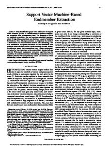
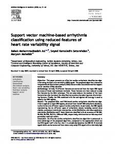
dictors for both in building the ensemble and testing it in the test set. As the SVM is a maximum margin classifier, which construct optimum separating hyperplane between the classes (for binary classification), we intend to use it in the first phase of the ensemble to attain the class posteriori probabilities consisting of the discriminative information between the classes and then integrate these as the additional predictors to construct the decision tree ensemble in the second phase. These posteriori probabilities are also used in the testing the decision tree ensembles. This procedure ensures a possibility of maximum separation of the classes and henceforth increases the prediction accuracy of the decision tree ensemble in discriminating the classes. Figure 1: Maximum Separation Hyperplane. In this paper, one of our main focus is to endeavor Double SVMBagging in classifying the type of partial discharge (PD) patterns in a model gas insulated switch gear (GIS) as a typical electric power apparatus. For condition monitoring purposes, it is considered to be important to identify the type of defects when monitoring discharge activities inside an insulation system. In the paper [17] authors first proposed to use the decision tree as a classification tool for diagnosing because it provides the tangible if-then-rule, and thus we may have a possibility to connect the physical phenomena to the observed signals. In [18] authors used several ensemble methods in classifying the defect patterns in the electric power apparatuses. In [27] authors applied a SVM ensemble for fault diagnosis, based on the genetic algorithm (GA). They used the GA in order to find more accurate and diverse ensemble. The paper is organized as follows. In section 2, we have introduced the SVM with a non-mathematical introduction and mathematical formulation, and then we have introduced some popular kernels we used in this paper in SVM. In section 3 we have introduced the double bagging and give a brief description of the implementation of the double bagging via the linear discriminant analysis (LDA). In section 4, the main topic of this paper is discussed: the Double SVMBagging. Here we have put together motivation and construction steps of Double SVMBagging. Section 5 contain the characteristics of the datasets used in the experiments. This also includes the extraction method used for the GIS datasets of the experiments in this paper. In section 6 the experimental setup of the study is explained, where we have compared the performance of the double bagging (with subbagging) SVM with other ensemble methods, such as the bagging, the adaboost.M1, the logitboost and the double bagging (with subbagging) with LDA and k-NN. In section 7 the results of the experiments are explained and discussed. In section 8, the conclusion of the study is stated.

2

Support Vector Machine (SVM)

The SVM models were originally defined for the classification of linearly separable classes of objects. Such an example is presented in Figure 1. For these two-dimensional objects that belong to two classes (class +1 and class −1), it is easy to find a line that separates them perfectly. For any particular set of two-class objects, an SVM finds the unique hyperplane having the maximum margin (denoted with δ in Figure 1). The hyperplane H1 defines the border with class +1 objects, whereas the hyperplane H2 defines the border with class −1 objects. Two objects from class +1 define the hyperplane H1 , and three objects from class −1 define the hyperplane H2 . These objects, represented inside circles in Figure 1, are called the support vectors. A special characteristic of the SVM is that the solution to a classification problem is represented by the support vectors that determine the maximum margin hyperplane. The SVMs aim at minimizing an upper bound of the generalization error through maximizing the margin between the separating hyperplane and the data. This can be regarded as an approximate implementation of the structural risk minimization (SRM) principle, which endows with good generalization performances independent of underlying distributions [21]. The SVMs algorithms are based on parametric families of separating hyperplanes of different Vapnik-Chervonenkis dimensions (VC dimensions). The SVMs can effectively and efficiently find the optimal VC dimension and an optimal hyperplane of that dimension simultaneously to minimize the upper bound of the expected risk. Usually the classification decision function in the linearly separable problem is represented by fw,b = sign(w · x + b). Thus, to find a hyperplane with minimum VC dimension, we need to minimize the norm of the canonical hyperplane ||w||. Also the distance between the hyperplane H1 and H2 showed in Figure 1 is, δ=

(Advance online publication: 22 May 2009)

2 . ||w||

Engineering Letter, 17:2, EL_17_2_09 ____________________________________________________________________________________

Consequently, minimizing the norm of the canonical hyperplane ||w|| is equivalent to maximizing the margin δ between H1 and H2 in Figure 1. The purpose of implementing SRM for constructing an optimal hyperplane is to find an optimal separating hyperplane that can separate the two classes of training data with maximum margin. In Figure 1, the support vectors construct these optimal hyperplanes. Hence the optimal hyperplane separating the training data of two separable classes is the hyperplane that satisfies, M inimize : F (w) =

1 T w w, yi (w · xi + b) ≥ 1. 2

This is a convex, quadratic programming (QP), problem with linear inequality constraints. It is hard to solve the inequality constraint optimization problem directly. The most common way to deal with optimization problems with inequality constraints is to introduce Lagrange multipliers to convert the problem from primal space to dual space and then solve the dual problem. For the linearly non-separable case, the minimization problem needs to be modified to allow the misclassified data points. This modification results in a soft margin classifier that allows but penalizes errors by introducing a new set of variables ξi (i = 1 . . . l) as the measurement of violation of the constraints. M inimize : F (w) =

L ∑ 1 T w w + C( ξi )k , 2 i=1

yi (wT φ(x) + b) ≥ 1 − ξi , where C and k are used to weight the penalizing variables ξi , and φ(·) is a nonlinear function which maps the input space into a higher dimensional space. Minimizing the first term in the above QP is corresponding to minimizing the VC dimension of the learning machine and minimizing the second term in QP controls the empirical risk. Therefore, in order to solve problem the QP, we need to construct a set of functions, and implement the classical risk minimization on the set of functions. Here, a Lagrangian method is used to solve the above problem. Then, the QP can be written as, after introducing L non-negative Lagrangian multipliers α1 , α2 , . . . , αL , M aximize : L(α), L L ∑ L ∑ 1∑ L(α) = αi − αi αj yi yj φ(x)T φ(xi )T , 2 i=1 i=1 j=1

subject to L ∑ i=1

αi yi = 0;

L ∑ i=1

αi ≤ C;

L ∑

αi ≥ 0.

i=1

After the optimum Lagrange multipliers αi have been determined, we can compute the optimum coefficient vector

w∗ and the optimal offset b∗ . The solution is given by L ∑ f (x) = sign( yi αi∗ (x) + b∗ ), i=1

αi∗ (x)

where = αi yi K(x, xi ), and K(x, xi ) = φ(x) · φ(xi ). (K(x, xi ) can be simplified by kernel trick [35]). One interesting property of support vector machines and other kernel-based systems is that, once a valid kernel function has been selected, one can practically work in spaces of any dimension without any significant additional computational cost, since feature mapping is never effectively performed. In fact, one does not even need to know which features are being used. Another advantage of SVMs and kernel methods is that one can design and use a kernel for a particular problem that could be applied directly to the data without the need for a feature extraction process. This is particularly important in problems where a lot of structure of the data is lost by the feature extraction process (e.g., text processing). In SVM for multi-class classification, mostly voting schemes such as one–against–one and one–against–all are used. In the one–against–one (classification method ) (also called pairwise classification), k2 classifiers are constructed where each one is trained on data from two classes. Prediction is done by voting where each classifier gives a prediction and the class which is most frequently predicted wins (“Max Wins”). In the one–against–all method k binary SVM classifiers are trained, where k is the number of classes, each trained to separate one class from the rest. The classifiers are then combined by comparing their decision values on a test data instance and labeling it according to the classifier with the highest decision value.

2.1

Kernels used in SVM

In this subsection, we present the most used SVM kernels. These functions are usually computed in a highdimensional space and have a nonlinear character. Linear (dot) kernel: The inner product of xi and xj defines the linear (dot) kernel K(xi , xj ) = xi · xj . This is a linear classifier, and it should be used as a test of the nonlinearity in the training set, as well as a reference for the eventual classification improvement obtained with nonlinear kernels. Polynomial Kernel: The polynomial kernel is a simple and efficient method for modeling nonlinear relationships: K(xi , xj ) = (1 + xi · xj )d . Gaussian Radial Basis Function: Radial basis functions (RBF) are widely used kernels, usually in the Gaussian

(Advance online publication: 22 May 2009)

Engineering Letter, 17:2, EL_17_2_09 ____________________________________________________________________________________

form:

||x − µ||2 K(xi , xj ) = exp( ). 2σ 2 The parameter σ controls the shape of the separating hyperplane. Exponential Radial Basis Function: K(xi , xj ) = exp(

||x − µ|| ). 2σ 2

Neural (tanh, sigmoid) kernel: The hyperbolic tangent (tanh) function, with a sigmoid shape, is the most used transfer function for artificial neural networks. The corresponding kernel has the formula: K(xi , xj ) = tanh(axi · xj + b). ANOVA Kernel: A useful function is the ANOVA kernel, whose shape is controlled by the parameters γ and d: ∑ K(xi , xj ) = ( exp(γ(xi − xj )))d . The Gaussian and Exponential RBF are general-purpose kernels used when there is no prior knowledge about the data. The linear kernel is useful when dealing with large sparse data vectors as is usually the case in text categorization. The polynomial kernel is popular in image processing and the sigmoid kernel is mainly used as a proxy for neural networks. The ANOVA RBF kernels typically perform well in regression problems. Usually RBFs are favored instead of polynomial kernel functions, because they are not sensitive to outliers and do not require inputs to have equal variances. However, in some cases polynomial kernels result in an excellent classification performance. In this paper we have used linear, polynomial, Gaussian radial basis function and sigmoid kernel.

2.2

Advantage of SVM over other classifiers in data based condition diagnosis

During the last years Neural Network (NN) based models like multilayer perceptrons (MLP), radial basis function (RBF) networks or self organising maps (SOM) in application to the data-based fault diagnosis is widely studied [37], [30]. With NN models it is possible to estimate a nonlinear function without requiring a mathematical description of how the output functionally depends on the input; NNs learn from examples. The most commonly mentioned advantages of NNs are their ability to model any non-linear system, the ability to learn, the highly parallel structure and the ability to deal with inconsistent or noisy data. But difficulties occur in creating a reliable network, if there are not enough measurements available from all operation states of the process. Another disadvantage of NNs is that the net architecture with weighting

factors is difficult to figure out by human. This may be a problem in tuning the system, or explaining the diagnosis results to a system operator. SVM gives refreshing views on conventional pattern recognition and classification systems. It has several benefits compared to statistical classifiers or MLPs, e.g. 1. The most important benefit is its efficiency in high dimensional classification problems, where statistical classifiers often fail. 2. The other benefit of SVM compared to statistical classifiers is its general applicability to nonlinear problems. MLPs or RBF networks can also be applied in nonlinear problems, but SVM outperforms them when considering the globality of solution. 3. Training of the SVM results in a global solution for the problem under study, whereas MLPs and RBF networks may have many local minima leading to not a reliable solution. Thus, we see that SVM possess some advantageous properties over other statistical classifiers not only in fault diagnosis but also in other real world classification problems. Our primary objective is to incorporate SVM in double bagging to utilize these advantages in fault diagnosis.

2.3

Designing and tuning of SVM in the experiments

We have used the C-SVM in our paper. This name originates from the fact that the complexity of the C-SVM solely depends on the cost parameter C. Design of SVM for a classification task consists of two tasks: choosing the kernel function and setting a value for the parameter C. The parameter C is also called an error penalty, because it deals with the trade-off between maximum margin and the classification error during training. A high error penalty will force the SVM training to avoid classification errors. It is clear that with high error penalty, the optimizer gives a boundary that classifies all the training points correctly. This, however, can give very irregular boundaries that may not lead good performance of the classifier in the test set. In this paper we have used the R package e1071 [7] to implement the SVM. In the SVMs the optimization is done by SMO [31], which takes advantage of the special structure of the SVM quadratic problem (QP). The selection of kernel function has also influence on the decision boundary. When using polynomial kernel function, the order of the polynomial needs to be chosen, and when using RBF the spread (kernel width) σ, needs to be decided. In our experiments we have used grid search method to select the optimum combination of the parameters. In this search method the 10-fold cross validation is used to search for the models with lowest

(Advance online publication: 22 May 2009)

Engineering Letter, 17:2, EL_17_2_09 ____________________________________________________________________________________

Input: • • • • •

L: Training set X: the predictors in the training dataset B: number of classifier in the ensemble {ω1 , . . . , ωc }: the set of class labels x: a data point to be classified

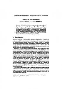
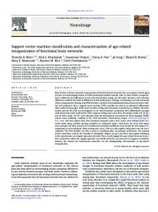
Training Phase: For b = 1, . . . , B • Draw a random sample L(b) with replacement from the training set L and (b) (b) where X (b) denote the matrix of predictors x1 , . . . , xN from L(b) . • Compute an LDA Z (b) , using the out-of-bag sample L−(b) , that gives a matrix W (b) where the columns are the coefficients of the linear discriminant functions. (b)

• Construct the combined classifier Ccomb using the original variables as well as the discriminant variables of the bootstrap sample (L(b) , X (b) W (b) ) Classification Phase: • For a new observation x, let cbj (x, xZ (b) ) be the decision(probability) as(b) signed by the classifier Ccomb to the hypothesis that x comes from the class ωj . Calculate the confidence for each class ωj , by the “average” combination rule: µj (x) =

B 1 ∑ cbj ((x, xZ (b) )), j = 1, . . . , c. B b=1

• Assign x to the class with the largest confidence. Figure 2: Double bagging Algorithm

prediction error. In our paper for multi-class classification we have used one–against–one rule. In all of our experiments we have used the posteriori class probabilities as output instead of class labels of SVM as the additional predictors. This is done by an improved implementation ([25]) of Platt’s a posteriori probabilities [32]. P rob(y = 1|f ) =

1 1+

e(Af +B)

where a sigmoid function is fitted to the decision values f of the binary SVM classifiers, A and B being estimated by minimizing the negative log-likelihood function. This is equivalent to fitting a logistic regression model to the estimated decision values. We extended the class probabilities to the multi-class case, combining all binary classifiers class probability output as proposed in [44]. As we have mentioned earlier in this section that SMO is used to optimize the parameters of the SVMs of our study, one can argue that, why not using other faster SVM implementations available (e.g., Bottou’s SVMSGD, Fan’s LINEARLIB [11], Chang’s PSVM [8]).

There are two reasons behind the expostulation to use faster SVMs: firstly, SMO is found to achieve better predictive performance considering speed, scalability and memory usage [22] than other contemporary SVM implementations in R language (see svmpath [15], klaR [34], kernlab [23], quadprog[42]), secondly we are using the SVM in the out-of-bag samples (which are 13 of each bootstrap sample), so in our understanding speeding up the learning process is less important here.

3

Double Bagging

When a decision tree is adopted as the base learning algorithm, only splits that are parallel to the feature axes are taken into account even though the decision tree is nonparametric and can be quickly trained. Considering that other general splits such as linear ones may produce more accurate trees, a “Double-Bagging” method is proposed by Hothorn and Lausen [19] to construct ensemble classifiers. In the statistical literature drawing a random sample of size N from the empirical distribution, a bootstrap sample of size N covers approximately 23 of the obser-

(Advance online publication: 22 May 2009)

Engineering Letter, 17:2, EL_17_2_09 ____________________________________________________________________________________

vations of the learning sample. The observations, which are not in the bootstrap sample, are called out-of-bag sample and may be used for estimating the misclassification error or for improved class probability estimates. In the double bagging framework proposed by Hothorn and Lausen [19], the out-of-bag sample is used to generate an additional classifier model to integrate with the base learning model. In the setup of Hothorn and Lausen, the double-bagging uses the values of the linear discriminant functions trained on the out-of-bag sample as additional predictors for bagging classification trees only. The discriminant variables are computed for the bootstrap sample and a new classifier is constructed using the original variables as well as the discriminant variables. The double bagging algorithm [19] is shown in Figure 2. Using the out-of-bag sample for the LDA, the coefficients of the discriminants are estimated by an independent sample; thus it is avoiding the overfitted discriminant variables in the tree growing process. Furthermore, it ensures that the training sample for the LDA is small and therefore the LDA becomes less stable and in the typical situation bagging can lead to stabilization. In double bagging, instead of the LDA, the other stable classifiers like, Nearest Neighbor (NN), Linear Logistic and SVM can be used as the additional classifier models.

4 4.1

Double Bagging with SVM The algorithm

The underlying idea of double bagging is in the spirit of Breiman [4], “Instead of reducing the dimensionality, the number of possible predictors available to the classification trees is enlarged and the procedure is stabilized by bootstrap aggregation.” In this algorithm a linear classifier model LDA is constructed for each bootstrap sample using an additional set of observations: the outof-bag sample. The prediction of this classifier is computed for the observations in the bootstrap sample and is used as additional predictors for a classification tree. The trees implicitly select the most informative predictors. The procedure is repeated sufficiently enough and a new observation is classified by averaging the predictions of the multiple trees. So we see that performance of the double bagging solely depends on two factors: 1) the classes of the dataset are linearly separable so that the additional predictors are informative (or discriminative), 2) the size of the out-of-bag samples as to construct LDA model: the underlying covariance matrix should be invertible. However, to handle real world classification problems, the base classifier should have more flexibility. In the next subsection we will discuss about the other possible classifier choices to use in double bagging and the advantage of SVM over them.

4.2

Other possible choices for additional classifier model in Double Bagging

In this subsection we will clarify our idea to select SVM as the additional classifier model in double bagging. The possible classifiers to be used other than LDA in the double bagging are, k-Nearest Neighbor (k-NN) classifiers, Neural Network (NN). We will discard NN from our discussion as SVM itself can be considered as a NN with radial basis function (RBF) while used with gaussian kernel. Below in brief we have stated the rationale behind not choosing of LDA and k-NN in using as the additional predictors in double bagging. Linear discriminant Analysis (LDA): We have seen in the earlier section that the success of double bagging depends on the linear structure in the dataset. But if there is no linear structure available in the datasets, we are adding some non-informative predictors in the ensemble construction. Furthermore it should be noted that for small learning samples with a large number of predictors, the out-of-bag sample may be too small for computing additional classifier LDA. On the contrary for a high dimensional dataset linear discriminant analyses apply the inverse of covariance matrix of the vectors to be classified requiring estimation of the covariance matrix. To estimate high dimensional covariance matrices well one needs an unpredictably large number of observations. So for using LDA we must ensure that the data is linearly distributed in the classes and also the dimension of the data generates invertible covariance matrix. k-Nearest Neighbor (k-NN): The nearest neighbor (NN) method is one of the simplest and well-known nonparametric classification methods. By the k-NN rule (k ≥ 1), to classify a new case with the feature variable values known, one simply looks at the k nearest neighbors in the available data and the class label with the highest frequency wins. For defining neighbors, a distance or metric is usually taken. So the performance of the NN method depends heavily on the chosen distance and distance metric. Given a set of feature variables, a key issue in the k-NN classification is the choice of the neighbor size k. Cover and Hart [10] showed that even 1-nearest neighbor rule can do half as well as the Bayes rule (the optimal classifier) in terms of the classification error probability. However, as the size of the training set becomes large, the computational time may become infeasible. In this paper we have used 5-NN and 10-NN as the additional classifiers condition diagnosis. The performance of double bagging with k-NN is competitive with double bagging with LDA in the experiments. From the above discussion it is clear that the use of SVM as an additional classifier in the double bagging will be beneficial because SVMs performance is compatible with the dimensionality of the dataset. The generalization ability of the SVM can be measured only with the num-

(Advance online publication: 22 May 2009)

Engineering Letter, 17:2, EL_17_2_09 ____________________________________________________________________________________

Input: • • • • •

L: Training set X: the predictors in the training dataset B: number of classifier in the ensemble {ω1 , . . . , ωc }: the set of class labels x: a data point to be classified

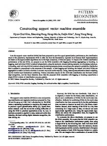
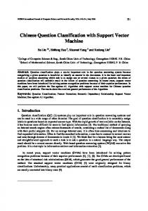
Training Phase: For b = 1, . . . , B • Draw a subsample L(b) without replacement of size 12 of the L. Let X (b) (b) (b) denote the matrix of predictors x1 , . . . , xN from L(b) . • Build an SVM model SV M (b) , using the out-of-bag sample L−(b) , train this model on L(b) , that gives a matrix CP (b) where the columns are the class probability of the classes of the dataset. (b)

• Construct the combined classifier Ccomb using the original variables (L(b) ) as well as the class probabability matrix (L(b) , CP (b) ) Classification Phase: • For a new observation x, let cbj (x, T CP (b) ) be the decision(probability) (b) assigned by the classifier Ccomb to the hypothesis that x comes from the (b) class ωj . Here T CP is the test set’s class posteriori probablity generated by SV M (b) . Calculate the confidence for each class ωj , by the “average” combination rule: B 1 ∑ cbj ((x, T CP (b) )), j = 1, . . . , c. µj (x) = B b=1

• Assign x to the class with the largest confidence. Figure 3: Double SVMSbagging Algorithm

ber of samples (Support Vectors) locating on the border of the classes regardless of the dimension of the input space. Also the computations are independent of the dimension of the input space, because they are handled through Gram matrices of the input data. The other benefit of SVM compared to statistical classifiers is its general applicability to nonlinear problems. Due to these reasons we have used SVM as the additional classifier. In addition to the above reasonings we also know that SVC (support vector classifier) are maximum margin classifier, i.e., the support vectors construct the separating hyperplane with the maximal margin between the classes (for example in 2-class problem), it has an extra advantage regarding automatic model selection in the sense that both the optimal number and locations of the support vectors are automatically obtained during training [36]. So in the double bagging the use of SVM will ensure that the additional predictors (the class posteriori probabilities) extracted after training the SVM models on the inbag samples, will consist of optimum discriminative

(maximal margin) information of the classes. Henceforth it will facilitate the base decision tree learn on the combined training sample (i.e., the bootstrap samples and the class posteriori probabilities) allow for more flexible and accurate split of the data. So it is evident theoretically that use of SVM in the double bagging therefore will have an improved performance. As the success of the double bagging mostly lies on the classifier model build on the out-of-bag samples, to ensure large out-of-bag samples we also used subsamples instead of the bootstrap samples, i.e., use 50% of each sample without replacement. We denote this as, “Double SVMSbagging”. This modification ensures that the learning samples for the additional classifier model always contain half of the observations of the training sample. This will be expedient in decreasing the probability of the additional classifiers to overfit the out of bag samples and also will increase the learning ability of the additional predictors.

(Advance online publication: 22 May 2009)

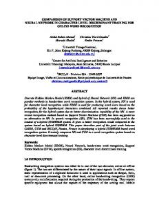
Engineering Letter, 17:2, EL_17_2_09 ____________________________________________________________________________________ Data Flow in Training phase Data Flow in Test phase

L1

O1

L2

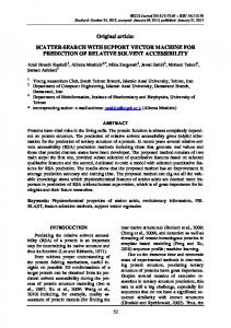
Lb = bth Bootstrap Sample Ob = bth Out of bag sample SVMb = SVM model built on Ob CPb = Class Posteriori Probabilities from Lb, after training SVMb on Lb TCP = Class Posteriori Probabilities from Test set, after training SVMb on Test set

Training Set

L

O2 … LB

OB

Multiple bootstrap Sets

Test SVM1

CP1

L1

DT1

SVM2

CP2

L2

DT2

Combine the DT using average rule

Training SVM using out-of-bag samples

SVMB

CPB

LB

Using these SVMs in Bootstrap samples and Test set Building DT ensemble with the SVs

DTB

Test

CCOMB

Test Set

, TCP1 …TCPB

Figure 4: Architecture of Double SVMBagging In Figure 3, we have given the pseudocode of Double SVMSbagging algorithm. For better understanding about the program flow of the Double SVMbagging ensemble we have also given Figure 4. So we see from Figure 4 that in the first phase of training step SVMs are constructed using the out-of-bag samples, then to get additional predictors, these SVMs are trained on the bootstrap samples to get the class posteriori probabilities (CP b ). In the second phase an ensemble of decision tree(DT b ) is built using these CP b s and the bootstrap samples (Lb ). The SVMs are also trained in the test set to enlarge the size of the test set by the test posteriori class probabilities (T CP b ). Then these TCPs are included with test set as the additional predictors. The SVM has been known to show a good generalization performance and is easy to learn exact parameters for the global optimum [6]. Because of these advantages, their ensemble may not be considered as a method for improving the classification performance greatly. However, since the practical SVM has been implemented using the approximated algorithms in order to reduce the computation complexity of time and space, a single SVM may not learn exact parameters for the global optimum. Sometimes, the support vectors obtained from the learning is not sufficient to classify all unknown test examples completely. So, we cannot guarantee that a single SVM always provides the global optimal classification performance over all test examples. This allows us to use the

SVM in bagging; as in bagging the base classifiers should be unstable to get better performance.

5

Data

The main objective of this paper is two fold; first, examine the performance of Double SVMBagging in condition diagnosis and compare its prediction accuracy with other ensemble methods; second, investigate its classification performance in real world datasets along with other wellknown ensemble methods. The datasets used for condition diagnosis are GIS (Gas Insulated Switchgears) datasets which are transformed version of the electromagnetic signals measured by the sensors in the electric power substations, since the stochastic signals measured cannot be used as they are because of too abundant information, they are once transformed into φ-V -n (phase resolved Partial Discharge (PD)) patterns. Then generalized normal distribution (GND) and Weibull distribution fitting [16] is used in order to acquire accurate diagnosis of the faults. We assume three classes for possible abnormal conditions in the GIS; 1) the metal which is attached on the high voltage side conductor (abbreviated as “HV”), 2) the metal which is attached on the earth side tank ((abbreviated as “TK”), and 3) the metal is freely movable (abbreviated as “FR”). The numbers of the observed samples are, 150, 377, 126, for HV, TK, FR. Here the first dataset consist of MLE

(Advance online publication: 22 May 2009)

Engineering Letter, 17:2, EL_17_2_09 ____________________________________________________________________________________

(Maximum Likelihood Parameters) of 4 parameters (2 parameters for phase 0-180 and 2 parameters for phase 180-360) of the GND and two parameters for the single phase of the Weibull fitted to the observed PD patterns, and these are used as feature variables. For our second experiment we randomely selected 15 datasets from the UCI Machine Learning Repository [1]. The characteristics of the datasets are showed in Table 1. Table 1: Description of the 15 Data used in this paper Dataset Boston Housing DNA Ecoli German-credit Glass Cleveland-Heart Ionosphere Iris Liver-disorder Pima-Diabetes Sonar Vehicle Vote Wiscinson-breast Zoo

Objects 506 3186 336 1000 214 297 351 150 345 768 208 846 435 699 101

Classes 3 3 8 2 7 5 2 3 2 2 2 4 2 2 7

Features 13 180 7 20 9 13 34 4 6 8 60 18 16 9 16

as a weak classifier to be used in boosting algorithms, we used it in the experiments. As there are three classes in the GIS datasets, to get reasonable results we have used here 3-node DS and 2-node DS. The results are shown in Table 2. In double bagging with SVM we have used four kernels (as stated in section 2.1) linear, polynomial, radial basis function and sigmoid. The main idea behind this is to check which kernel produces better diagnosis results. In our earlier experiments [17], [45] we split the dataset into two independent parts, one for training, the training set (50% of the dataset) and the test set (remaining 50% of the data). We performed this splitting 5, 10, 25 and 50 times in order to avoid the dependence on the splitting. In this experiment we have used 10-fold crossvalidation to estimate the misclassification error of the ensemble methods. We repeat this 5 times and report the average misclassification error of the 5 repititions. In [17] and [45] the accuracy of the bagging and double bagging ensemble was better with the ensemble size B = 100, for that the ensemble size for bagging and double bagging ensemble is 100 in all the experiment in this paper; in case of adaboost.M1 and logitboost we have used iterations M = 100. We have reported in Table 2 the lowest test errors of the classifiers. The best result is printed in bold. In the first column of Table 2 we have given the name of the ensemble methods and in the second column we have given the abbreviations we have used for the ensemble methods. For example for a Bagged CART ensemble we have used “BCART”. In Table 2 we see that for the GND fitted dataset, the per-

6

Experimental Setup and Discussion of formance of BCART is (misclassification error 4.4%) better than single CART and adaboost.M1 and logitboost. results

In this paper we have conducted two experiments. In the first experiments we have applied Double SVMBagging in the two GIS datasets. To compare the efficacy of the proposed double bagging via SVM ensemble we have performed three different ensemble methods, bagging [3], adaboost.M1 [12] and logitboost [13], with the double bagging (with subbagging) with LDA, 5-NN and 10-NN classifier models. In the second experiment we have checked the performance of the new ensemble method in 15 UCI repository datasets. We have compared its perfromance with Bagging, Adaboost.M1, Random Forest [5] and Rotation Forest [33]. In all the experiments for each dataset, we extracted the optimum parameters of the SVM using 10-fold crossvalidation and then use those parameters to construct the SVC to be used in each out of bag sample.

6.1

Experiment with GIS dataset

In the first experiment, we have used CART [2] in bagging, double bagging and adaboost.M1 and decision stump (DS) [20] in adaboost.M1 and logitboost as the base classifier. We used here 2-node decision stump in case of adaboost.M1 and logitboost and 3-node decision stump in case of adaboost.M1. Since DS is more efficient

We see that 3-node DS has the highest prediction accuracy among the boosted algorithms. Among the results of DB5NN, DB10NN, DBLDA, DSB5NN, DSB10NN and DSBLDA we see that DBLDA has the highest accuracy than the other classifier (accuracy 96.02%) although DB5NN has 95.11% accuracy. We see here that the accuracy has increased (or misclassification error is decreased) than the best acquired by BCART (accuracy 95.6%). From the results of the double bagging (and subbagging) via the SVM, we see that the better performing SVM for this data is the RBF, as the DBRBF and DSBRBF have the lowest misclassification error (0.03198, 0.02885) among all the classifiers here. The main reason for the success of the RBF kernel to perform very well could be that we used the Gaussian RBF instead of the exponential RBF and as the features of this dataset are the fitted parameters of generalized normal distribution, and the kernel function mapped the features in the best way than the other kernel methods. We also see that all the classifiers instead of DSBPOLYSV and DSBLINSV produced error nearly the same or lower than the other classifiers. For the Weibull fitted GIS dataset we see that the double bagging (also subbagging) with 5-NN has the highest ac-

(Advance online publication: 22 May 2009)

Engineering Letter, 17:2, EL_17_2_09 ____________________________________________________________________________________

Table 2: Misclassification error of all the ensemble methods for GND and Weibull fitted GIS dataset Classifiers

Abbreviations

GND fitted Data

Weibull fitted Data

CART BCART

0.08638 0.04407

0.08191 0.03891

Double Bagging With LDA, 5-NN and 10-NN DBLDA DB5NN DB10NN DSBLDA DSB5NN DSB10NN

0.03798 0.03889 0.04610 0.04086 0.03824 0.04314

0.03730 0.03316 0.04315 0.04097 0.03439 0.04271

Double Bagging With SVM DBLINSV

0.03811

0.04221

DBPOLYSV

0.03425

0.03524

DBRBFSV

0.03198

0.03442

DBSIGSV

0.03795

0.04349

DSBLINSV

0.04284

0.04037

DSBPOLYSV

0.03591

0.03600

DSBRBFSV

0.02885

0.03543

DSBSIGSV

0.03891

0.03914

Boosting Methods ADACART ADADS2

0.05238 0.09687

0.04717 0.09587

ADADS3

0.04671

0.04518

LOGITDS

0.07221

0.03492

Single Decision Tree Bagged CART Double Double Double Double Double Double

bagging with LDA bagging with 5-NN bagging with 10-NN subbagging with LDA subbagging with 5-NN subbagging with 10-NN

Double bagging with linear kernel SVM Double bagging with polynomial kernel SVM Double bagging with RBF kernel SVM Double bagging with sigmoid kernel SVM Double subbagging with linear kernel SVM Double subbagging with polynomial kernel SVM Double subbagging with RBF kernel SVM Double subbagging with sigmoid kernel SVM Adaboost.M1 CART Adaboost.M1 Decision Stump with 2-node Adaboost.M1 Decision Stump with 3-node LogitBoosted Decision Stump

curacy (96.84% and 95.61%). The double bagging with RBF kernel performed better among the double bagging with SVM. It acquired 34.42% and 35.43% misclassification error which is better than all classifiers except, DB5NN, DSB5NN. The performance of LOGITDS is satisfactory in this dataset, it is the fourth best performer (error 34.92%) in this dataset. The performance of polynomial SVM kernel like the GND fitted dataset, better than linear and sigmoid kernel double bagging SVM classifiers. So wee see that in both the GIS dataset the performance of the double bagging SVM classfiers with RBF and Polynomial kernel performed very well in classifying the abnormal conditions. In Weibull fitted dataset, however, the accuracy of double bagging with 5-NN is better than double bagging with RBF and polynomial SVM kernel.

6.2

Experiment with the UCI dataset

In this section we describe our findings of the comparative experiment with our new ensemble creation technique and several ensemble creation technique of CART (Bagging, Adaboost, Random Forest (abbreviated as Rand-

Forest in the table) and Rotation Forest (abbreviated as RotForest in the table). For each data set and ensemble method, five 10-fold cross validations were performed. The average accuracies and the standard deviations are reported in Table 3. In this experiment for each data set, we used stratified ten-fold cross-validation method. A stratified n-fold cross-validation breaks the data set into n disjoint subsets each with a class distribution approximating that of the original data set. For each of the n folds, an ensemble is trained using n − 1 of the subsets, and evaluated on the held out subset. As this creates n non-overlapping test sets, it allows for statistical comparisons between approaches to be made. We used t-test for testing the statistical significance of the observed differences in errors of the ensemble methods. In this approach a t-test is conducted on the results of a ten-fold cross validation. This is the most widely used approach for this type of experiment. While the ten folds of the crossvalidation have independent test sets, the training data is highly overlapped across folds, and use of the t-test assumes independent trials. The results for which a significant difference with double bagging with RBF SVM is found are marked with a

(Advance online publication: 22 May 2009)

Engineering Letter, 17:2, EL_17_2_09 ____________________________________________________________________________________

Table 3: Mean and Standard deviations prediction error of single CART, Bagged CART, Adaboost CART,Double Bagged CART,Random Forest and Rotation Forest Dataset Boston Housing DNA Ecoli German-credit Glass Cleveland-Heart Ionosphere Iris Liver-disorder Pima-Diabetes Sonar Vehicle Vote Wiscinson-breast Zoo Win–Tie–Loss

Single 0.2623 ± 0.013 • 0.0921 ± 0.014 • 0.1934 ± 0.019 • 0.3580 ± 0.137 • 0.2561 ± 0.066 • 0.3250 ± 0.048 • 0.1126 ± 0.059 • 0.0556 ± 0.010 0.3604 ± 0.013 • 0.3451 ± 0.017 • 0.3104 ± 0.018 • 0.2948 ± 0.011 • 0.0675 ± 0.010 0.0595 ± 0.001 • 0.1237 ± 0.018 • 13–2–0

Bagging 0.2176 ± 0.012 0.0452 ± 0.017 0.1786 ± 0.011 • 0.2914 ± 0.064 0.2595 ± 0.058 • 0.2214 ± 0.043 • 0.0655 ± 0.037◦ 0.0470 ± 0.012 0.3172 ± 0.014 • 0.2811 ± 0.029 • 0.2088 ± 0.014 0.2546 ± 0.012 0.0460 ± 0.014 0.0298 ± 0.004 0.1074 ± 0.030 • 5–9–1

AdaBoost 0.2148 ± 0.014 0.0428 ± 0.019 0.1636 ± 0.018 0.2677 ± 0.051 0.2568 ± 0.049 • 0.2127 ± 0.042 • 0.0681 ± 0.036◦ 0.0516 ± 0.015 0.3151 ± 0.019 • 0.2433 ± 0.028 0.1834 ± 0.024 0.2387 ± 0.015 0.0517 ± 0.012 0.0430 ± 0.010 • 0.0575 ± 0.027 • 5–9–1

Double Bagging 0.2156 ± 0.018 0.0434 ± 0.015 0.1541 ± 0.016 0.2788 ± 0.067 0.2364 ± 0.052 0.1837 ± 0.041 0.0786 ± 0.039 0.0490 ± 0.011 0.2896 ± 0.021 0.2430 ± 0.022 0.2083 ± 0.029 0.2401 ± 0.017 0.0490 ± 0.011 0.0343 ± 0.001 0.0401 ± 0.029

RandForest 0.2195 ± 0.011 0.0532 ± 0.023 • 0.1631 ± 0.016 0.2756 ± 0.089 0.2645 ± 0.058 • 0.1994 ± 0.064 0.0716 ± 0.039 0.0500 ± 0.009 0.3078 ± 0.026 • 0.2755 ± 0.027 • 0.1852 ± 0.017◦ 0.2470 ± 0.018 0.0509 ± 0.013 0.0320 ± 0.002 0.0498 ± 0.032 4–10–1

RotForest 0.2118 ± 0.029 0.0418 ± 0.020 0.1582 ± 0.017 0.2895 ± 0.081 • 0.2549 ± 0.034 • 0.1893 ± 0.064 0.0621 ± 0.036◦ 0.0440 ± 0.010 0.3051 ± 0.025 • 0.2553 ± 0.028 0.1820 ± 0.030◦ 0.2226 ± 0.011◦ 0.0422 ± 0.010 0.0288 ± 0.006 0.0782 ± 0.030 • 4–8–3

“•” indicates Double Bagging is significanly better, “◦” indicates Double Bagging is significanly worse at the significance level α = 0.05

bullet or an open circle next to them. A bullet next to a result indicates that double bagging with RBF SVM is significantly better than the respective method (column) for the respective data set (row). An open circle next to a result indicates that double bagging with RBF SVM is significantly worse than the respective method. In the triplet labeled, “Win–Tie–Loss” in the last row of Table 3, the first value is the number of data sets on, the double bagging with RBF SVM is significantly better than the other ensemble methods; the second one is the number of data sets on which the difference between the performance of the double bagging with RBF SVM and that of the other ensemble methods is not significant; the third one denotes the number of data sets on which the double bagging with RBF SVM is significantly worse than the other ensemble methods. We see from Table 3 that double bagging with RBF SVM performed consistently better than Bagging, Adaboost and Random Forest in the datasets. The Rotation Forest due to its ingenious construction has performed better than our method in the datasets.

7

Conclusions

CART searches for partitions in the multivariate samples space, which may be seen as higher-order interactions or homogeneous subgroups defined by some combination binary splits of the predictors. SVM has advantage over other classifiers in (a) non-linear feature space, (b) dimensionality of the feature space and (c) generalization ability. In adition to these SVC construct the optimum separating hyperplane which maximize the margin between the classes (in binary classification). To build an

ensemble of classifier with better generalization performance we combine these two methods. A new SVM ensemble method has been proposed in this study, being a variant of another ensemble method named double bagging, where the SVM is used to construct additional classifier models using an independent sample than the training sample (the out-of-bag sample) to enhance the generalization performance of the ensemble method. Then, these additional predictors are combined with the CART to build the ensemble. The new method is used to detect the defects in the insulation system in order to model a better diagnosis system for the electric power apparatus. The proposed method outperformed other ensemble methods such as bagging, adaboost.M1, logitboost and double bagging with LDA and k-NN (k = 5 and 10), in the experiments. The new method is found to be better than most of the other ensemble classifier methods in diagnosing abnormal states. The new double bagging method with RBF kernel SVM is tested on several UCI datasets and its performance is consistently better than popular ensemble methods like bagging, boosting and random forest. Its performance is also competitive with the recent ensemble method roation forest. In our future work we intend to construct a double bagging with localized version of the additional classifier, which will ensure better discriminative information for the primary base classifier (which is the decision tree in our case). It should be noted that prunning this new double bagging ensemble method is also an interesting area of the research.

(Advance online publication: 22 May 2009)

Engineering Letter, 17:2, EL_17_2_09 ____________________________________________________________________________________

References [1] C. L. Blake and C. J. Merz, UCI Repository of Machine Learning Databases, 1999, http://www. ics.uci. edu/mlearn/MLRepository.html. [2] L. Breiman, J.H. Friedman, R.A. Olshen, and C.J. Stone, Classification and Regression Trees, Belmont, CA:Wadsworth, 1984. [3] L. Breiman, Bagging predictors, Machine Learning, 24(2):123–140,1996. [4] L. Breiman, Statistical modeling: the two cultures, Statist. Sci., 16(3),199–231 (with discussion), 2001. [5] L. Breiman, Random Forests, Machine Learning, 45(1), 5–32, 2001. [6] C. J. C. Burges, A Tutorial on Support Vector Machines for Pattern Recognition, Data Min. Knowl. Discov., 2, 121–167 1998. [7] C. C. Chang, C. J. Lin, libsvm: A Library for Support Vector Machines, 2001. [8] Y. E. Chang, K. Zhu, H. Wang, H. Bai, J. Li, Z. Qiu, H. Cui, PSVM: Parallelizing Support Vector Machines on Distributed Computers, NIPS, 2007. [9] C. Cortes and V. Vapnik, Support-Vector Networks, Mach. Learn., 20, 273–297 1995. [10] T. M. Cover, and P. E. Hart, Nearest neighbor pattern classification, IEEE Transactions on Information Theory, 13, 21–27, 1967. [11] R. E. Fan, K. W. Chang, C. J. Hsieh, X. R. Wang, and C. J. Lin, LIBLINEAR: A library for large linear classification, Journal of Machine Learning Research, 9, 1871–1874, 2008. [12] Y. Freund and R. Schapire, Experiments with a New boosting algorithm, Machine Learning: Proceedings to the Thirteenth International Conference, Morgan Kaufmann, San Francisco, 148–156, 1996.

[16] H. Hirose, S. Matsuda and M. Hikita, Electrical Insulation Diagnosing using a New Statistical Classification Method, In the Proceedings of 8th Internal Conference on Properties and Applications of Dielectric Materials (ICPADM2006), 698–701, 2006. [17] H. Hirose, M. Hikita, S. Ohtsuka, S. Tsuru and J. Ichimaru, Diagnosing the Electric Power Apparatuses using the Decision Tree Method, IEEE Trans., Dielectrics and Electrical Insulation, 15(5), 1252– 1261, 2008. [18] H. Hirose, F. Zaman, K. Tsuru, T. Tsuboi, and S. Okabe, Diagnosis Accuracy in Electric Power Apparatuses Conditions using the Classification Methods, IEICE Technical Report, 108(243), 39–44, 2008. [19] T. Hothorn and B. Lausen, Double-bagging: combining classifiers by bootstrap aggregation, Pattern Recognition,36 (6), 1303–1309, 2003. [20] W. Iba and P. Langley, Induction of one-level decision trees, In Proceedings of Ninth International Machine Learning Conference, Aberdeen, Scotland. 1992. [21] T. Joachims, Making large-scale support vector machine learning practical, Advances in Kernel Methods: Support Vector Machines, MIT Press, Cambridge, MA, 1999. [22] A. Karatzoglou, A. Smola, K. Hornik, Support Vector Machines in R , Journal of Statistical Software, Volume 15(9), 1–28, April 2006. [23] A. Karatzoglou, A. Smola, K. Hornik, A. Zeileis, kernlab ? Kernel Methods, R package, Version 0.6-2, 2005. [24] H. C. Kim, S. Pang, H. M. Je, et al., Constructing support vector machine ensemble, Pattern Recognition, 36(12), 2757–2767, 2003. [25] H. T. Lin, C. J. Lin and R. C. Wen (2001), A Note on Platt?s Probabilistic Outputs for Support Vector Machines, 2001.

[13] J. Friedman, T. Hastie, and R. Tibshirani, Additive logistic regression: a statistical view of boosting, Annals of Statistics, 28, 337–407(with discussion), 2000.

[26] K. Li, Y. Dai, W. Zhang, Ensemble Implementations on Diversified Support Vector Machines, In the Proceeding of IEEE Fourth International Conference on Natural Computation, 180–184, 2008.

[14] T. V. Gestel, J.Suykens, B.Baesens, S. Viaene,J. Vanthienen, G. Dedene, B. D. Moor, and J. Vandewalle, Benchmarking least squares support vector machine classifiers, Machine Learning, 54(1), 5–32, 2001.

[27] Y. Li, Y. Cal, R. Yin, X. Xu, Fault diagnosis based on support vector machine ensemble, In Proceedings of 2005 International Conference on Machine Learning and Cybernetics, 6, 3309–3314,18-21 Aug. 2005.

[15] T. Hastie, svmpath: The SVM Path algorithm, R package, Version 0.9, 2004.

[28] J. Min, J. Hong, and S. Cho, Ensemble Approaches of Support Vector Machines for Multiclass Classification,

(Advance online publication: 22 May 2009)

Engineering Letter, 17:2, EL_17_2_09 ____________________________________________________________________________________

[29] D. Meyer, F. Leisch, and K Hornik, The support vector machine under test, Neurocomputing, 55:169– 186, September 2003.

[42] A. Weingessel, quadprog ? Functions to Solve Quadratic Programming Problems, R package, Version 1.4-7, 2004.

[30] R. J. Patton, C. J. Lopez-Toribio, F. J. Uppal, Artificial Intelligence Approaches to Fault Diagnosis., Condition Monitoring, IEE Colloquium on Machinery, External Structures and Health (Ref. No. 1999/034), 5/1–5/18, 1999.

[43] J. Weston, C. Watkins, Support vector machines for multi-class pattern recognition, Proceedings of the Seventh European Symposium on Artificial Neural Networks, Bruges, Belgium, 1999.

[31] J. Platt, Fast Training of Support Vector Machines Using Sequential Minimal Optimization In Advances in Kernel Methods - Support Vector Learning, B. Scholkopf, C. J. C. Burges, and A. J. Smola, Eds., MIT Press, Cambridge, Massachusetts, 185–208, 1999. [32] J. C. Platt, Probabilistic Outputs for Support Vector Machines and Comparison to Regularized Likelihood Methods, In A Smola, P Bartlett, B Sch?olkopf, D Schuurmans (eds.), Advances in Large Margin Classifiers, MIT Press, Cambridge, MA, 2000.

[44] T. F. Wu, C. J. Lin and R. C. Weng, Probability Estimates for Multi-class Classification by Pairwise Coupling, Advances in Neural Information Processing, 16, 2003. [45] F. Zaman, and H. Hirose, A New Double Bagging via the Support Vector Machine with Application to the Condition Diagnosis for the Electric Power Apparatus, International Conference on Data Mining and Applications(ICDMA’09), 654–660, 2009.

[33] J. J. Rodr´ıguez, L. I. Kuncheva, and C. J. Alonso, Rotation forest: A new classifier ensemble method, IEEE Transaction on Pattern Analysis and Machine Intelligence, 28(10),1619–1630, 2006. [34] C. Roever, N. Raabe, K. Luebke, U. Ligges, klaR ? Classification and Visualization, R package, Version 0.4-1, 2005. [35] B. Scholkopf, A. Smola , and K. Muller, Nonlinear component analysis as a kernel eigenvalue problem, Neural Computation, 10(5),1299–1319,1998. [36] B. Scholkopf, C. J. C. Burges, and A. J. Smola, Advances in Kernel Methods: Support Vector Learning, MIT Press, Cambridge, Massachusetts, 1999. [37] T. Sorsa, Neural Network Approach to Fault Diagnosis, Doctoral Thesis, Tampere University of Technology Publications 153, 1995. [38] B. Sun, D. Huang, Least squares support vector machine ensemble, In Proceedings of IEEE International Joint Conference on Neural Networks, 3, 2013–2016, 2004. [39] V. Vapnik. The Nature of Statistical Learning Theory,Springer, New York, 1999. [40] G. Valentini, T. Dietterich, Low bias bagged support vector machines, In 20th International Conference on Machine Learning,T. Fawett, N. Mishra (Eds),Washington DC, USA, 2003. [41] G. Yan, G. Ma, and L. Zhu, Support Vector Machines Ensemble Based on Fuzzy Integral for Classification, ISNN 2006, J. Wang et. al (eds.), LNCS 3971, 974–980, 2006.

(Advance online publication: 22 May 2009)