A Novel Robust Method for Large Numbers of. Gross Errors. Hanzi Wang and David Suter, Senior Member, IEEE .... probability density function (PDF) around the.
Seventh International Conference on Control, Automation, Robotics And Vision (ICARCV’02), Dec 2002, Singapore
A Novel Robust Method for Large Numbers of Gross Errors Hanzi Wang and David Suter, Senior Member, IEEE Department of Electrical and Computer Systems Engineering Monash University, Clayton Vic. 3800, Australia. {hanzi.wang ; d.suter}@eng.monash.edu.au The contributions of this paper can be summarized as follows : (1) We provide a novel estimator which can tolerate more than 85% outliers. (2) We apply nonparametric density estimation and density gradient estimation techniques in parametric estimation. Instead of considering residuals as the only feature, both the density distribution of data points and the residual corresponding to the local maximum density distribution are considered as features in our objective function. (3) MDPE can deal with the data with multistructured outliers. This paper is organized as follows: in section 2, we review previous methods and their limits. The density gradient estimation and mean shift method are introduced in section 3. In section 4, we describe MDPE method. Experimental results are contained in section 5. Finally, we conclude with a discussion of further possible work.
Abstract In computer vision tasks, it frequently happens that gross noise occupies the absolute majority of the data. Most robust estimators can tolerate no more than 50% gross errors. In this article, we propose a highly robust estimator, called MDPE (Maximum Density Power Estimator), employing density estimation and density gradient estimation techniques in the residual space. This estimator can tolerate more than 85% outliers. Experiments illustrate that the MDPE has a higher breakdown point and less errors than other recently proposed similar estimators: Least Median of Squares (LMedS), Residual Consensus (RESC), and Adaptive Least kth Order Squares(ALKS). 1.Introduction There has recently been a general recognition in computer vision community that algorithms should be robust because it is unavoidable that data are contaminated (due to faulty feature extraction, sensor noise, segmentation errors, etc). The outliers may include uniformly distributed, or clustered outliers or pseudo-outliers (arising from multiple structures). Thus outliers may occupy the absolute majority of the data. In this paper we introduce a new estimator (MDPE). The goals in designing MDPE were: it should be able to fit signals corresponding to less than 50% of the data points, and fit data with multi-structures. We assume the inliers occupy a relative majority (instead of the absolute majority which is assumed in general estimators such as the LMedS and the LTS [5]) of the data points. Probability Density estimation and Mean Shift techniques [13] are employed in MDPE. The mean shift vector always points towards the direction of the maximum increase in the probability density function. Through the mean shift iterations, the local maximum density, corresponding to the mode (or the center of the regions of high concentration) of data, can be found. Two criteria are considered in our objective function: • The density distribution of the data points provided by the density estimation technique. • The value of the residual corresponding to the local maximum of probability density. If the signal is correctly fitted, the densities of inliers should be as large as possible; at the same time, the value of the center of the high concentration of data should be as close to zero as possible in the residual space.
2. Previous methods and their limitations. Great efforts have been made in the search for high breakdown point estimators in recent decades. The maximum-likelihood-type estimators (M-estimators) [2][3] are well-known among the robust estimators. Although M-estimators can reduce the influence of outliers, they have breakdown points less than 1/(p+1), where p is the number of the parameters to estimate: robustness diminishes when the dimension p increases. Siegel [4] proposed the repeated median (RM) estimator with the breakdown point of 50%. However, the time complexity of the repeated median estimator is O(nplogpn), which prevents the method being useful in applications where p is even moderately large. Rousseeuw [5] proposed the least median of squares (LMedS) method. The LMedS finds the parameters to estimate by minimizing the median of residuals corresponding to the data points. The LMedS also has a breakdown point of 50% (except in extreme situations where it may breakdown earlier). When the outliers are more than 50% of the data, the LMedS method will fail completely to fit a model. The RESC [8] method can tolerate more than 50% outliers. RESC uses a compressed histogram method to infer residual consensus. However, RESC needs the user to tune parameters in the procedure for
326
compressing the histogram and in its objective function for optimal performance. The authors of MUSE [10] and those of ALKS [11] consider robust scale estimate and they both obtain a breakdown point higher than 50%. However, MUSE needs a lookup table for the scale estimator correction; ALKS is limited in its ability to handle extreme outliers.
The mean shift vector Mh(x) is defined as: 1 1 M h (x) ≡ ∑ ( X i − x) = n X ∈∑S ( xX) i − x n x X i ∈Sh ( x ) x i h Then, equation (4) can be rewritten as:
M h (x) ≡
if x T x < 1
(6)
Equation (6) first appeared in [13]. Equations (5) shows that the mean shift vector is the difference between the local mean and the center of the window; and equations (6) shows that the mean shift vector is an estimate of the normalized density gradient. The Mean Shift algorithm can be simply described as follows: 1. Initialize the location of the searching window x0 and yk= x0, (k=1). 2. Compute yk+1= 1 ∑ X , k=k+1. Repeat i nk X i ∈Sh ( yk ) until convergence. The converged centers (or windows) correspond to modes (or centers of the regions of high concentration) of data represented as arbitrary-dimensional vectors. The proof of the convergence of the mean shift algorithm can be found in [16][17]. To illustrate the mean shift method, two normal distributions are generated, each having 1000 data points and with unit variance. One has a distribution with zero mean, and the other has a mean of 4.0 (see figure 1). We selected two initial points: P0 (-2.0) and P1 (2.5). The search window radius was chosen as 1.0. After applying mean shift algorithm, the mean shift estimator automatically found the local maximum densities (converged points). Precisely, P0’ located at 0.0305, and P1’ with 4.0056. The centers (P0’ and P1’) of the converged windows correspond to the local maximum probability densities, that is, the two modes.
3. Density Gradient Estimation and Mean shift Method When a model is correctly fitted, there are two criteria that should be satisfied: (1) Data points on or near the model (inliers) should be as many as possible, i.e., the probability density function (PDF) around the model should be as high as possible; (2) The residuals of inliers should be as small as possible. Our new method, MDPE, considers these two criteria in its objective function and it employs density estimation and density gradient estimation techniques. The accuracy of density estimation and density gradient estimation will directly affect the achievements of MDPE in fitting models. There are several nonparametric methods available for probability density estimation: histogram, naive method, the nearest neighbor method, and kernel estimation [12]. The kernel estimation method is one of the most popular techniques used in estimating density. Given a set of n data points {Xi}I=1,…,n in a d-dimensional Euclidian space Rd, the multivariate kernel density estimator with kernel K and window radius (band-width) h is defined as follows [12, p.76] x − Xi 1 n (1) fˆ ( x) = d ∑ K ( ) h nh i =1 The kernel function K(x) should satisfy some conditions [18, p.95]. There are several different kinds of kernels. The Epanechnikov kernel [12, p.76] is one optimum kernel which yields minimum mean integrated square error (MISE): 1 −1 T c (d + 2)(1 − x x) K e ( x) = 2 d 0
ˆ f ( x) h2 ∇ d + 2 fˆ ( x)
(5)
(2)
otherwise
where cd is the volume of the unit d-dimensional sphere, e.g., c1=2, c2=π, c3=4π/3. The estimate of the density gradient can be defined as the gradient of the kernel density estimate (1) ˆ f ( x) ≡ ∇fˆ ( x) = 1 ∇ nhd
n
∑ ∇K ( i =1
x − Xi ) h
(3) Fig.1 One example where the mean shift estimator found the local maximum of the probability densities.
According to (3), the density gradient estimate of the Epanechnikov kernel can be rewritten as: d +2 1 (4) ˆ f ( x) = n x ( X i − x) ∇ ∑ d 2 n( h c d ) h n x X i ∈Sh ( x ) where the region Sh(x) is a hypersphere of the radius h, having the volume
4. Maximum Density Power Estimator 4.1 The density power (DP) We assume the residuals of the inliers (good data points) satisfy a Gaussian-type distribution. If the model to fit is correctly estimated, the data points on or near
h d c d , centered at x, and containing
nx data points.
327
the primitive should have a higher probability density; at the same time, the center of the converged window by the mean shift procedure (corresponding to the highest local probability density) should be as close to zero as possible. According to the above assumptions, our objective function ψDP considers two factors: (1) the
Experiments, presented next, will show MDPE is a very powerful method for data with a large percentage of outliers. 4.2 The MDPE algorithm The MDPE adopts a multistep procedure: (1) Initialize a search window radius h, and a repetition count m. (2) Randomly choose one p-subset, estimate the model parameters by the p-subset, and calculate the signed residuals of all data points. (3) Apply the mean shift iteration in the residual space with initial window center zero. (4) Calculate the densities corresponding to the positions of all data points within the converged window with radius h. (5) Calculate the density power according equation (7). (6) Repeat step (2) to step (5) m times. Finally, output the parameters with maximum density power. The results are determined by one p-subset (of m psubsets), corresponding to the maximum density power. In order to improve the statistical efficiency, a weighted least square procedure [1, p.202] can be carried out after the initial MDPE fit.
densities fˆ (Xi) of all data points within the converged window Wc and (2) the center C of the converged window. Thus ψDP
∑ fˆ ( X
∝
X i ∈Wc
i
) and ψDP ∝
1 . C
We define the probability density power function as: fˆ α ( X i ) ∑ ψDP = X i ∈Wc (8) β k+C where C is the center of the converged window Wc obtained by applying the mean shift procedure; α , β and k are the parameters that adjust the relative influence of the probability density and the residual of the point corresponding to the center of the converged window. They are empirically set for the best achievements. For our case, they are set 1.0, 1/3 and 1.0. If a model is found,
C is very small, and the densities
within the converged window are very high. Thus our objective function will get a highest score. Vice versa. 1 00
100
90
90
80
80 RESC
70
70 60
LM ed S
A LK S
60 ALKS 50
50 40
LMedS
40
RESC
30
30
20
M DPE
20
MDPE
10
10
0
0 0
10
20
30
40
50
60
70
80
90
0
100
10
20
30
(a)
40
50
60
70
80
90
100
(b)
100
100 90
90 MDPE 80
RESC
80
RESC
70
70
60
60
50
50
MDPE
40
40
LMedS
ALKS
30
30
20
20
10
10
0 0
10
20
30
40
50
60
70
ALKS
80
90
LMedS
0
100
0
10
20
30
40
50
60
70
80
90
100
(c) (d) Fig. 2. Four examples for comparing the performance of four methods: (a) fitting a step with total 87% outliers; (b) fitting three steps with total 91% outliers; (c) fitting a roof with total 93% outliers; (d) fitting six lines with total 94% outliers.
328
MDPE to fit circles under 95% outliers. Five circles were generated, each with 100 data points and σ=0.1. 1500 random outliers were distributed at range (-75 75). H was set 7.0. Thus, for each circle, it has 1900 outliers (400 pseudo-outliers plus 1500 random outliers). This figure contained a multiple-solution type of data. As a result, the MDPE method gave the most accurate results of the four methods.
5. Experiments and Analysis In this section, we will compare the abilities of MDPE, RESC, ALKS, and LMedS to deal with data with a large percentage of outliers. The factors affecting the mean number of iterations in mean shift are investigated. Unless we specify the window radius h, it is set at 2.0. Experiment 1. We generated four kinds of data (step, three-step, roof, and six-line), each with a total of 500 data points. The signals were corrupted by Gaussian noise with zero mean and standard variance σ. Among the 500 data points, α data points were randomly distributed in the range of (0, 100). The ith structure has γi data points. (a) Step: x:(0-55), y=30, γ1=65; x:(55-100), y=40, γ2=30; α=405; σ=1. (b) Three-step: x:(0-30), y=20, γ1=45; x:(30-55), y=40, γ2=30; x:(55-80), y=60, γ3=30; x:(80-100), y=80, γ4=30; α=365; σ=1. (c) Roof: x:(0-55), y=x+30, γ1=35; x:(55-100), y=140x, γ1=30; α=435; σ=1. (d) Six-line: x:(0-25), y=3x, γ1=30; x:(25-50), y=1503x, γ2=20; x:(25-50), y=3x-75, γ3=20; x:(50-75), y=3x-150, γ4=20; x:(50-75), y=225-3x, γ5=20; x:(75-100), y=300-3x, γ6=20; α=370; σ=0.1. From figure 2, we can see that because LMedS has only a 0.5 breakdown point, it cannot resist more than 50% outliers. Thus, LMedS failed to fit all the four signals; The ALKS, RESC and MDPE approaches all have a more than 50% breakdown point. But the results show that ALKS is not appropriate for the signals with a very large percentages of outliers because it failed in all four cases. In contrast, the RESC successfully fitted three models, but failed one. Only the MDPE correctly fitted all the four signals. The MDPE didn’t breakdown even with 94% outliers.
Experiment 3. One aspect in the implementation of MDPE is the convergence speed of the mean shift. The convergence speed of the mean shift will directly affect the efficiency of MDPE. When the initial center of the searching widow is set in a region of high density value, the mean shift convergence is quick and the mean shift step is small; on the other hand, if the initial window is chosen near the a low density region, the convergence is poor and the mean shift step is large. The mean number of iterations needed to guarantee to convergence is related to the choice of window radius: if the searching window radius is large, more data points will fall into the searching window. As a result, the mean number of iterations will be large. 2.6
6 5.5
2.4
Mean Number of Iterations
Mean Shift Iterations
5 4.5 4 3.5 3 2.5 2
2.2
2
1.8
1.6
1.5 1 0
1.4
100
200
300 400 500 600 700 800 Times of Randomly Sampling p-subsets
900 1000
2
4
6
8 10 Window Radius h
12
14
(a) (b) Fig. 4 (a) the number of mean shift iterations in 1000 residual-density spaces determined by randomly sampling p-subsets. (b) the relationship between the mean number of iteration and the searching window radius h.
Experiment 2.
From Figure 4 (a) we can see that the number of mean shift iterations in different residual-density spaces, which are determined by the data points and randomly chosen p-subsets, is different. But the mean number of mean shift iterations will increase with the enlargement of the searching window radius due to more data points included in the searching window, which is shown in figure 4 (b) (we repeated the result 20 times). Experiment 4. Although the MDPE has showed its powerful ability to tolerate large percentage of outliers (including pseudooutliers), its success is decided by the correct choice of window radius h. If h is chosen too small, it is possible that the densities of data points in the residual space may not be corrected estimated (the density function is a noisy function with many local peaks and valleys), and some inliers is possibly neglected; on the other hand, if h is set too large, the window will include all the data
Fig. 3. One example of fitting circles by the four methods. The data had 95% outliers. The MDPE is a general method that can be easily extended to fit other kinds of models, such as circles, ellipsis, planes, etc. Figure 3 shows the ability of the
329
The first example is to fit a line in the pavement shown in figure 6. The edge image was obtained by using Canny operator with threshold 0.15 and included 2213 data points (shown in figure 6 (b)). There were about 85% outliers (most belonging to pseudo-outliers which had structures and belonged to other lines) in the data. Four methods (MDPE, RESC, ALKS, and LMedS) were applied to fit a line in the pavement. As shown in figure 6(c), both MDPE and RESC correctly found a line in the pavement. However, ALKS and LMedS failed to correctly fit the line. The second example is to fit a circle edge of one cup out of twelve cups. Among the total 1959 data points, the inliers corresponding to each cup were less than 10% of the total data points. This is a multiple-solution case: the fitted circle can correspond to any cup in the twelve cups. As shown in figure 7, only MDPE correctly found the cup edge. However, all other three methods failed to fit the circle edge of the cup.
points including inliers and outliers; all peaks and valleys of the density function will also be smoothed out. Figure 5 shows that the errors in A and B increase with the window radius h for the cases where 60%, 70% and 80% percentage of uniformly distributed outliers were added to the signal. This is because when the radius becomes larger, it is possible that more outliers were included within the converged window. But the influence of different window radii on the results is small for different percentage of outliers when the h is within a certain range, for example, for this case, when h is set within the range at (1-15), the results will not be affected greatly. At the same time, the percentage of outliers also has influence on the sensitivity of the results to the choice of window radius. The more percentage of outliers, the more influence of changing window radii on results. 25
0.2 60% Outliers 70% Outliers 80% Outliers
0.1
60% Outliers 70% Outliers 80% Outliers
20
0
Error in B
Error in A
15
-0.1
-0.2
10
5
-0.3 0
-0.4
-5
-0.5 0
5
10
15 Window Radius h
20
25
30
0
5
10
15 Window Radius h
20
25
30
220
(a) (b) Fig. 5.The influence of window radius and percentage of outliers on the results of the MDPE.
200 180 160 140 120 100 80
Experiment 5. In this experiment, we will give two real images to show the ability of MDPE to tolerate large percentage of outliers. The window radius was set 2.0 (for line fitting) and 7.0 (for circle fitting).
(a)
60 40 20 0
(a)
50
100
150
200
250
(b)
(b)
ALKS
LMedS
(c) Fig. 7 Fitting a circle edge. (a) twelve cups; (b) the edge image by using Canny operator; (c) the results of circle fitting obtained by four methods.
MDPE and RESC
(c) Fig 6. Fitting a line (a) one real pavement; (b) the edge image by using Canny operator; (b) the results of line fitting obtained by four methods.
5. Discussion In this paper, we provide a novel robust estimator, MDPE, to fit models. We randomly choose m p-subsets,
330
[7] H. Wang and D. Suter, “ Using Symmetry in Model Fitting,” Submitted to IEEE Trans. Pattern Analysis and Machine Intelligence. [8] X. Yu, T.D. Bui, and A. Krzyzak, “Robust Estimation for Range Image Segmentation and Reconstruction,” IEEE Trans. Pattern Analysis and Machine Intelligence, 16(5), pp.530-538, 1994 [9] C.V. Stewart, “MINPRAN: A New Robust Estimator for Computer Vision,” IEEE Trans. Pattern Analysis and Machine Intelligence, 17(10), pp.925-938, 1995 [10] J.V. Miller and C.V. Stewart, “MUSE: Robust Surface Fitting Using Unbiased Scale Estimates,” Proc. Computer Vision and Pattern Recognition’96, pp.300306, San Francisco, June, 1996. [11] K-M Lee, P. Meer, and R-H Park, “ Robust Adaptive Segmentation of Range Images,” IEEE Trans. Pattern Analysis and Machine Intelligence, 20(2), pp.200-205, 1998 [12] B.W. Silverman, Density Estimation for Statistics and Data Analysis, London: Chapman and Hall, 1986. [13] K. Fukunaga and L.D. Hostetler, “The Estimation of the Gradient of a Density Function, with Applications in Pattern Recognition,” IEEE Trans. Info. Theory, vol. IT-21, pp. 32-40, 1975. [14] Y. Cheng, “Mean Shift, Mode Seeking, and Clustering,” IEEE Trans. Pattern Analysis and Machine Intelligence, 17(8), pp.790-799, 1995. [15] ] D. Comaniciu and P. Meer, “Robust Analysis of Feature Spaces: Color Image Segmentation,” ,” in Proceedings of 1997 IEEE Conference on Computer Vision and Pattern Recognition, San Juan, PR, , pp.750755, June 1997. [16] D. Comaniciu and P. Meer, “Mean Shift Analysis and Applications,” in Proceedings 7th International Conference on Computer Vision, Kerkyra, Greece, pp.1197-1203, September 1999. [17] D. Comaniciu and P. Meer, “Mean Shift: A Robust Approach towards Feature Space Analysi,” To appear in IEEE Trans. Pattern Analysis and Machine Intelligence,2001 [18] M. P. Wand and M. Jones, Kernel Smoothing, Chapman & Hall, 1995. [19] M. A. Fischler and R. C. Rolles, “Random Sample Consensus: A Paradigm for Model Fitting with Applications to Image Analysis and Automated Cartography,” Commun. ACM, 24(6), pp.381-395, 1981. [20] K. Fukunaga, Introduction to Statistical Pattern Recognition, Boston: Academic Press, 1990.
calculate residuals for each p-subset, apply the mean shift procedure to find the local maximum density, and output the estimated parameters determined by one psubset corresponding the maximum density power. MDPE can tolerate more than 85%, even more than 90%, outliers. MDPE does not require that the outliers are uniformly distributed — the outliers can have structure. MDPE only requires that the inliers occupy the relative majority of the data points. MDPE can be used to fit the data with outliers that are uniformly distributed, have multiple-structure, and/or are clustered (not very dense). MDPE has obtained excellent achievements in situations with very large percentage of outliers. The procedure of the density estimation and the mean shift in MDPE is unsupervised. No user input is required. A crucial parameter we need to choose is the window radius h. Normally, the method will be stable for a reasonable range, when the window radius is changed from small to large [20, p.541]. Thus, the optimal window radius can be decided by the center of the largest operating range that yields the same parameters for a given data. When the percentage of outliers is very large or there are many structures in the data, one problem in carrying out any method which uses random sampling is: the number of p-subsets , m, to be sampled, is huge when the percentage of outliers ε is large. For example, if we require that the probability to have at least one “clean” p-subset is 0.95, and if the percentage of contaminated data ε is 90%, then the times (m) that p-subsets need to be sampled is 2994 for p=3; and 2995700 for p=6! If ε is more than 90%, the m will increase more quickly with ε and p. Thus, a more feasible technique for sampling p-subsets is needed for fitting a data with a large number percentage of outliers and multiple structures. Acknowledgement This work is supported by the Australia Research Council (ARC), under the grant A10017082. References [1] P.J. Rousseeuw, and A.Leroy, Robust Regression and outlier detection, John Wiley & Sons, New York, 1987 [2] P.J. Huber, “Robust Regression: Asymptotics, Conjectures and Monte Carlo,” Annals of Statistics, 1, pp.799-821, 1973. [3] P.J. Huber, Robust Statistics, New York, Wiley, 1981. [4] A.F.Siegel, “Robust Regression using Repeated Medians,” Biometrika, 69, pp.242-244, 1982 [5] P.J. Rousseeuw, “Least Median of Squares Regression,” J. Amer. Stat. Assoc. 79, pp. 871-880, 1984 [6] L.S. Davis (Ed), Foundations of Image Analysis, pp.323-347, Kluwer, 2001.
331