A PROBE based heuristic for Graph Partitioning - UEA

1

A PROBE based heuristic for Graph Partitioning Pierre Chardaire, Musbah Barake, and Geoff P. McKeown

Abstract— A new heuristic algorithm, PROBE BA, based on the recently introduced metaheuristic paradigm PROBE (Population Reinforced Optimization Based Exploration) is proposed for solving the Graph Partitioning Problem. The “exploration” part of PROBE BA is implemented using the Differential-Greedy algorithm of Battiti and Bertossi and a modification of the Kernighan and Lin algorithm at the heart of Bui and Moon’s Genetic Algorithm, BFS GBA. Experiments are used to investigate properties of PROBE and show that PROBE BA compares favourably with other solution methods based on Genetic Algorithms, Randomized Reactive Tabu Search, or more specialized multilevel partitioning techniques. In addition, PROBE BA finds new best cut values for 10 of the 34 instances in Walshaw’s Graph Partitioning Archive. Index Terms— Evolutionary computing, heuristic methods, graph algorithms, graph bisection, graph partitioning.

L

I. I NTRODUCTION

ET G = (V, E) be an undirected graph, where V = {v1 , v2 , ..., vn } is a set of n vertices, E is a set of edges connecting the vertices, and C = (cij ) is the adjacency matrix of G, i.e., cij = 1 if there is an edge between i and j, otherwise cij = 0. The cardinality of E is denoted by e. The set of neighbours of a vertex vi is denoted by Γ(vi ), and is formally defined as Γ(vi ) = {vj | {vi , vj } ∈ E}. The Graph Bisection Problem (GBP), also known as the Graph Bipartitioning Problem, consists of partitioning V into two disjoint subsets A and B with cardinalities differing by at most one unit while minimizing the total number of the edges connecting the vertices in the two subsets. The two subsets (A, B) form a bisection of G and the set of edges connecting them is called a cut. The cut value is calculated by X T (A, B) = cab , a ∈ A and b ∈ B. We will assume that the number of vertices in the graph is even, as we can always add a vertex connected to no other vertices without changing the problem. In this case the subsets A and B have the same cardinality. Problems of graph partitioning arise in various areas of computer science, including sparse matrix factorization [1], VLSI design [2], [3], parallel computing [4]–[8], and data mining [9]. In particular the bisection problem is used in VLSI circuit placement to model the placement of “standard cells” to minimize the “routing area” used to connect the cells [10] and in physics to find the ground state magnetization of spin glasses [11]. M. Barake is with the School of Business, Center for Advanced Mathematical Sciences, American University of Beirut, P.O. Box 11-0236, Bliss Street, Beirut, Lebanon.E-mail: [email protected] P. Chardaire and G. P. McKeown are with the School of Computing Sciences, University of East Anglia, Norwich, NR4 7TJ, UK. E-mail: {pc,gmp}@cmp.uea.ac.uk

The GBP has been extensively studied in the past [12], [13]. The problem is NP-hard [14]. Therefore, the only practical methods that have been developed for the solution of instances of non-trivial sizes are of heuristical nature. Some of these methods use general metaheuristic paradigms for combinatorial optimization such as Simulated Annealing [15], Tabu Search [16]–[18], Genetic Algorithms [19], [20], Greedy Randomized Adaptive Search (GRASP) [21]. Other heuristics are specifically designed for the particular problem being solved. The most popular of these heuristics is the Kernighan-Lin algorithm (KL) [12]. This is a group migration algorithm which starts with a bisection and improves it by repeatedly selecting an equal-sized vertex subset in each side and swapping the two sets. Such heuristics are often the basis for metaheuristic solution specializations. Recently multilevel algorithms have been developed to solve problems of very large size. These multilevel algorithms approximate the original graph by a sequence of increasingly smaller graphs. The smallest graph is then partitioned using an efficient technique, and this partition is propagated back through the sequence of graphs and refined. Multilevel techniques have been proposed in [22]–[26]. Walshaw [27] makes a case for the use of multilevel refinement as a metaheuristic for the solution of combinatorial problems. Multilevel techniques are usually much faster than metaheuristic-based algorithms but do not always compete in terms of solution quality. Some of these techniques were developed for the fast preprocessing of data in parallel calculation. The objective in some practical applications is not necessarily to find optimal solutions but to find reasonably good solutions within short computing times. The recent algorithm TPART developed by Saab [26] seems to be able to find good solutions (within a few percent of the best known solution) rapidly as well as high quality solutions (best known or very close to best known) if enough time is allocated to the method (more iterations.) II. M OTIVATION Our motivation in this research was to test a new metaheuristic technique we had recently proposed. This metaheuristic christened PROBE (for Population Reinforced Optimization Based Exploration) is population based but is simpler than Genetic Algorithms as it does not include concepts of selection, mutation, and replacement. The basic idea of PROBE is to use a population to determine subspaces that are explored to find optimized solutions. These optimized solutions form a new population and the process is repeated. Our interest in the GBP stems from the work of Bui and Moon [19] and the work of Battiti and Bertossi [18], [28] on this problem. In particular, Bui and Moon designed a GA to

2

which our method could be compared, and Battiti and Bertossi designed a greedy algorithm useful to the implementation of a PROBE based solution method. The Breadth First Search Genetic Bisection Algorithm (BFS GBA) of Bui and Moon [19] solves the GBP by using a hybridized, steady-state, genetic algorithm with multi-point crossover. Solutions are coded as bit strings with a one-toone correspondence between bits and vertices. The value of a bit in the string indicates whether a vertex is in one side of the bisection or in the other, thus a string that has as many zeros as ones lead to a feasible solution. The fitness of each chromosome varies linearly with the cut value of the solution. At each iteration a biased selection towards the fitter chromosomes is performed to pick two parents from the population. Two offspring solutions are generated by first applying crossover and mutation. This generally leads to infeasible solutions that are repaired by using a simple scheme of flipping bits. The better of the two solutions is then passed to a linear time implementation of the KernighanLin algorithm. The final solution obtained replaces the closest parent with respect to its Hamming distance, but only if it has a better solution value. The algorithm stops when 80% of the solutions in the population have the same solution value. An important aspect of Bui and Moon’s algorithm is a preprocessing phase that uses breadth first search to reorder the vertices in an attempt to ensure that clusters of tightly connected vertices are included in short schemas that have more chance to survive a crossover operation. Battiti and Bertossi proposed a number of Tabu Search algorithms for the GBP [18]. Their first algorithm, Fixed Tabu Search (FIXED-TS), starts from an initial bisection and improves upon it by a scheme of local search and prohibition. Details about FIXED-TS and discussion of the relationship between prohibition and KL can be found in [17]. At each iteration, a vertex is selected from one side of the bisection, moved to the other side, and is prohibited to move back again for a certain number of iterations (prohibition parameter). The input bisection to FIXED-TS is obtained by running Battiti and Bertossi’s Min Max greedy construction algorithm which builds a bisection by alternatingly adding one vertex to each partition in a greedy manner. A number of experiments were carried out and suggested that the prohibition parameter had a big effect on the quality of the solution obtained but unfortunately there appeared to be no trivial way of obtaining the best parameter value for each instance of the graphs. To solve this problem Battiti and Bertossi proposed a randomized version where the problem of parameter tuning is solved by repetitive call to the FIXED-TS algorithm with the prohibition parameter generated at random at each call. Finally, in their Reactive Randomize Tabu Search (RRTS) algorithm they used a combination of randomization and reactive approaches. Basically the method exploits information from previous runs to self-tune its parameter of prohibition. (see [18] for details.) In Section III we present the PROBE metaheuristic. In Section IV we describe our specialization of PROBE to the solution of the GBP. Finally in Section V we test our method experimentally on benchmark problem instances and compare it with Bui and Moon’s BFS GBA, Battiti and Bertossi’s

RRTS, and Saab’s TPART. III. PROBE: P OPULATION R EINFORCED O PTIMIZATION BASED E XPLORATION PROBE is a population based metaheuristic that has recently been proposed by Barake, Chardaire and McKeown [29]. PROBE directs optimization algorithms, general or specific, towards good regions of the search space using some ideas from genetic algorithms (GAs) [30]. An important property of the (standard n-point) crossover operator used in GAs is that if two parents share a common bit value their offspring inherits it. PROBE uses this characteristic to generate feasible offspring from feasible parents. PROBE maintains, at each generation g, a population of feasible solutions Sig , i = 0, 1, . . . , P − 1. The next generation of solutions is obtained as follows. For each i = 0, . . . , P − 1 the solution, Sig+1 , g is computed from the pair (Sig , Si+1 ) (where the subscripts are taken modulo P ) by the sequence of steps in Figure 1. In this figure the term vector of components represents any Input:

A population of solutions represented as a vector of components Sig , i = 0, . . . , P − 1.

Output: A population of solutions represented as a vector of components Sig+1 , i = 0, . . . , P − 1. SPg ←− S0g . for i from 0 to P − 1 do g 1) Fix the components that have the same value in Sig and Si+1 .

2) Find an instantiation of the remaining components using an appropriate search algorithm. 3) Use the instantiation obtained as a starting point for a local optimizer. The solution obtained is Sig+1 . end do return (Sig+1 , i = 0, . . . , P − 1). Fig. 1.

Generation of solutions in PROBE

appropriate coding of the solution, such as bit string or table of integers. It is clear that step 1 guarantees that the subspace searched in step 2 contains a feasible solution if both parent solutions are feasible. The PROBE basic scheme can be refined to allow control of the size of the space searched in step 1 (see [29] for details.) However these refinements are not used in our implementation for the GBP. Details of our implementation for the GBP are provided in Section IV. A. A Theoretical Property of PROBE An interesting feature of the PROBE meta-heuristic is that when the selected subspace search algorithm is an exact algorithm, the above version of PROBE guarantees that the average fitness of the solutions in the pool increases until all solutions have the same fitness. Proposition 1: Let Fig be the fitness (objective value to be maximized) of solution of index i mod P in generation g and

3

let

P −1 1 X g F A = P i=0 i g

be the average fitness of the pool of P solutions in generation g. If the subspace search algorithm used by PROBE is an exact algorithm then Ag+1 > Ag , unless all solutions at generation g have the same fitness. Proof: Assume with no loss of generality that F0g 6= F1g . If F0g < F1g then F0g+1 ≥ max(F0g , F1g ) > F0g . Moreover, g+1 g Fi ≥ max(Fig , Fi+1 ) ≥ Fig for i = 1 . . . P − 1. Hence, g+1 g A >A . If F0g > F1g then F0g+1 ≥ max(F0g , F1g ) > F1g . Moreover, g g Fig+1 ≥ max(Fig , Fi+1 ) ≥ Fi+1 for i = 1 . . . P − 1. Hence, g+1 g A >A . Corollary 1: Under the hypothesis of proposition 1 PROBE converges to a population of solutions which all have the same fitness. Proposition 1 gives some theoretical foundation to the method even if practical implementations of PROBE do not generally meet the hypothesis of proposition 1. Our PROBE implementation for the GBP does not meet the hypothesis of proposition 1 as it does not use an exact algorithm for subspace search. However, we shall see in Section V-B that its runs converge for the instances tested. IV. A P ROBE BASED S OLUTION M ETHOD FOR THE GBP In this section we detail our implementation of PROBE for the GBP (PROBE BA for PROBE Bisection Algorithm.) GeneratePopulation (S g ) Input:

A population of solutions represented as a vector, S g , of bit strings Sig , i = 0, . . . , P − 1. Output: A population of solutions represented as a vector, S g+1 of bit strings Sig+1 , i = 0, . . . , P − 1. SPg ←− S0g ; for i from 0 to P − 1 do 1) (Ai , Bi ) ← Decode (Sig ); g (Ai+1 , Bi+1 ) ← Decode (Si+1 ); A ← Ai ∩ Ai+1 ; B ← Bi ∩ Bi+1 ; 2) /* construction phase */ (A, B) ← DifferentialGreedy (A, B); 3) /* local optimization phase */ (A, B) ← BuiAndMoonKL (A, B); Sig+1 ← Encode (A, B); end do return (S g+1 ); Fig. 2. Algorithm Generate Population: Generation of solutions in PROBE BA

Each solution to the GBP is represented by a binary string which corresponds to a bisection of the graph. The number of bits in the solution equals n, the number of vertices in the graph. Each bit corresponds to a vertex in the graph. A bit has a value 0 if the corresponding vertex is in one side of the bisection, and has a value 1 otherwise. One of the bits, say,

the first one could be fixed to one to eliminate symmetrical solutions. Preliminary experimental results indicated however that it is slightly better not to use this scheme. The fitness is the cost of external links of the bisection and is to be minimized. PROBE BA starts with a population, S 0 , of feasible solutions generated randomly and independently. The solutions are placed in the population in the order they are generated (i.e., solution of index 0 is generated first, solution of index P − 1 is generated last.) PROBE BA iterates the algorithm in Figure 2 for a maximum number of generations (user parameter MAXITER) or until no improvement on the best cut value has been found for a number of generations (user parameter STUCK.) The function Decode(s) decodes a binary string, s, into an array of vertex labels whereas the function Encode performs the inverse operation. In the following subsections we examine the implementation of steps 2 and 3 of the algorithm. A. Construction of a subspace solution An interesting feature of the GBP is that any two solutions share as many bits fixed to one as they do bits fixed to 0. More formally we have the following proposition: Proposition 2: Assume that (A, B) is a bisection of a graph, G, where vertices in A are labelled with 0 and vertices in B are labelled with 1. In the same way, assume that (C, D) is a bisection of G where vertices in C are labelled with 0 and vertices in D are labelled with 1. Then the number of vertices with the same label 0 in the two bisections is equal to the number of vertices with the same label 1 in the two bisections. Proof: |A ∩ C| + |A ∩ D| = |A| = n/2 ⇒ |A ∩ C| = n/2 − |A ∩ D| and |B ∩ D| + |A ∩ D| = |D| = n/2 ⇒ |B ∩ D| = n/2 − |A ∩ D| The result follows. We determine a solution in the subspace defined by the two parent solutions by using a greedy algorithm (if the two parent solutions are identical there is only one such solution.) As shown by proposition 2, a partially constructed solution to the bisection problem with as many vertices on each side of the partial bisection can be found by fixing the vertices corresponding to the bits shared by the two parent solutions. The corresponding partial bisection is used as input to the Differential-Greedy algorithm of Battiti and Bertossi [28] to produce a bisection of the full graph. The basic idea of the Differential-Greedy algorithm is to construct a bisection (A, B) by adding vertices alternately to the two sets in a greedy fashion. At each stage the vertex selected to enter a set, say the set A, is the vertex for which the number of neighbour vertices in A (internal degree) minus the number of neighbour vertices in B (external degree) is maximum. If several vertices are candidates to enter a set one of these vertices is selected at random. An outline of the algorithm is presented in Figure 3. The rationale behind the vertex selection criterion is that a bisection that minimizes

4

the cut size also maximizes the number of internal edges. In large graphs with low density the choice criterion used is better than one solely based on the external degree of the vertices, in particular if the algorithm is initialized with a small partial bisection. Indeed, in such a case many vertices have an external degree of zero for a large number of iterations of the algorithm. Input:

A graph, G = (V, E), with |V | mod 2 = 0. A partial bisection (A0 , B0 ) with |A0 | = |B0 |

Output: A bisection (A, B) of G. Initialize bisection with A ← A0 and B ← B0 ,; Initialize the set of remaining vertices: R ← V − (A ∪ B); while (R 6= ∅) do SelectPa vertex, x ∈PR, that maximizes b∈B Cxb ; a∈A Cxa − R ← R − {x}; A ← A ∪ {x}; SelectPa vertex, x ∈PR, that minimizes b∈B Cxb ; a∈A Cxa − R ← R − {x}; B ← B ∪ {x}; end while return (A, B); Fig. 3.

The Differential-Greedy algorithm.

Note that the Differential-Greedy algorithm as presented in [28] starts with one vertex in each side of the bisection (these two vertices are selected at random.) In our solution method we use the Differential-Greedy algorithm to construct solutions from partial bisections. The Differential-Greedy algorithm is also implemented using a bucket array structure. It is not difficult to establish that when this structure is used the computational complexity of the algorithm is O(e) (see [28] for example.) B. Local Optimizer Once a solution has been constructed an improvement phase is applied. In our solution method we use a local optimizer designed by Bui and Moon [19] for their Genetic Algorithm. This local optimizer is based on the Kernighan and Lin algorithm (KL) [12]. The main feature of KL is its capability of escaping local optima by accepting non-improving moves, only if they contribute later to a better cut value. KL takes as input an initial bisection generated at random and improves upon it by swapping equal-sized subsets to create a new bisection. The process is repeated on the new bisection until no improvement can be obtained. Given a bisection (A, B), KL orders the elements of A and B using the following method: For every pair of vertices (a, b) ∈ A × B let g(a, b) represent the reduction in cut value obtained upon swapping the two vertices. It is easy to see that g(A, B) = Da + Db − 2cab where Dx represents the cut value reduction obtained when x is moved to the other side of the partition. Dx is called the

difference value (or D value) of vertex x. KL selects the pair (a1 , b1 ) which maximizes g(a, b). Once a1 and b1 are selected, they are assumed to be exchanged and not considered any more for further exchange. The process is repeated to produce a sequence of pairs (a1 , b1 ), . . . , (an/2−1 , bn/2−1 ). Then KL Pk selects t ∈ argmaxk R(k) where R(k) = i=1 g(ai , bi ). If R(t) > 0 an improved bisection, ((A−Xt )∪Yt , (B−Yt )∪Xt ) with Xt = {a1 , . . . , at } and Yt = {b1 , . . . , bt }, is obtained. KL has a theoretical worst complexity of O(e.n3 ) as the maximum number of passes that might be considered is bounded by e (since each pass reduces the cut size by at least one unit and the size of the initial bisection is at most e) and the complexity of each pass is O(n3 ). Nevertheless, researchers have empirically shown that the number of passes does not exceed 10 in most cases, thus the typical practical complexity of KL is O(n3 ) (see [19] for more details). The basic idea of the local optimizer proposed by Bui and Moon had already been proposed by Kernighan and Lin [12]. Instead of examining all pairs of vertices eligible for exchange at each iteration of a pass of KL only a small number of pairs are examined using the following method: Two vertices with largest D values in A are selected from that set. Then two vertices are selected from B in a similar way. The best pair amongst the four resulting combinations is selected for exchange. Bui and Moon use a bucket array structure to store vertices according to their D values. This reduces the complexity to O(e). In addition they perform a single pass of this algorithm and limit the number of swapped pairs to a parameter. The rational is to avoid premature convergence in their GA. They found that setting the parameter to bn/6c gave the most desirable overall performance for their algorithm on the graphs they tested. In all our experiments we use the same choice of the parameter. V. N UMERICAL E XPERIMENTS In all our experiments the CPU times of our algorithm is given for a DELL Optiplex GX260, with Pentium 4, 2.391 GHz processor and 670 MB of usable RAM. Our programs are written in C++ and compiled under Microsoft Visual C++ using the standard release option (i.e., with optimizations performed on a per module basis only.) We compare our results with those published by Bui and Moon [19], by Battiti and Bertossi [18], and by Saab [26]. CPU times for Bui and Moon’s BFS GBA, Battiti and Bertossi’s RRTS, and Saab’s TPART were obtained on a Sun Sparc IPX, a Digital AlphaServer 2100 Model 5/250, and a Compaq Alpha DS20E 67/667 Mhz respectively. Battiti and Bertossi estimated that their machine is 12.7 times faster than Bui and Moon’s. Our machine’s architecture is similar to that of a Dell Precision Worstation 350, 2.4 GHz P4, whose SPECint2000 base rate is 9.05 which makes it approximately 2.7 times faster than a Dell precision 420 dual 733 MHz processor with 512 Mbytes of RAM. The SPECint95 benchmark indicates that the latter is 5.9 faster than Battiti and Bertossi’s machine. Hence our machine is approximately 16 times faster than Battiti and Bertossi’s, and 203 times faster than Bui and Moon’s. The SPECint2000 base rate for Saab’s machine is 4.93 indicating

5

that our machine is approximately 1.8 times faster than his. These coefficients have been used to scale other authors’ computing times in our tables of results. Our main interest is in establishing whether a PROBEbased solution method can compete in terms of solution quality rather than in finely comparing computing times, as long as the computing time is reasonable and does not grow too fast with the problem instance size. The computational tests are executed on three groups of graphs. The first group is composed of 16 graphs proposed by Johnson et al. [15] and 24 graphs proposed by Bui and Moon [19]. It contains the following types of graphs: • Gn.d: A random graph with n vertices, where an edge between any two vertices is created with probability p such that the expected degree, p(n − 1) of a vertex is d, • Un.d: A random geometric graph with n vertices uniformly distributed in the unit square. Two vertices are connected with an edge if and onlypif their Euclidean distance is less than or equal to d/(nπ). d is the expected vertex degree. • breg.n.b: A random regular graph with n vertices of degree 3, whose optimal bisection size is b with probability 1 − o(1). See [31]. • cat.n: A caterpillar graph with n vertices. It is constructed by starting with a path (the spine.) Each vertex on the spine is then connected to six new vertices, the legs of the caterpillar. With an even number of vertices on the spine, the optimal bisection size is 1. • rcat.n: A caterpillar graph with n vertices, where each √ vertex on the spine has n legs. These graphs have optimal bisection size of 1. • grid.n.b: A grid graph with n vertices, whose optimal bisection size is b. • w-grid.n.b: The same grid graph as above, but the boundaries are wrapped around. The second group contains graphs related to applications in parallel computing. It contains four numerical grids (airfoil1, big, wave, nasa4704), two graphs that belong to the Harwell-Boeing collection [32] (bcspwr09, bcsstk13), and two De Bruijn networks (DEBR12, DEBR18.) These graphs can be obtained from the Graph Partitioning Repository at the University of Paderborn (Internet address: http://wwwcs.uni-paderborn.de/ fachbreich/AG/monien/RESEARCH/PART/graphs. html.) Their dimensions are shown in Table I. Finally the last group is composed of the 34 graphs in Walshaw’s Graph Partitioning Archive [33] at the University of Greenwich (Internet address: http://staffweb. cms.gre.ac.uk/%7Ec.walshaw/partition/.) They represent a sample of real-world applications from various origins. The dimensions of the graphs are shown in Table II. In Section V-A we examine the impact of the strict ordering of solutions in the populations of PROBE BA. In Section V-B we experimentally establish the convergence of the algorithm. Section V-C shows the influence of the population size on solution quality. Section V-D examines whether it is a better

Graph airfoil1 big wave nasa4704 bcspwr09 bcsstk13 DEBR12 DEBR18

Number of vertices 4253 15606 156317 4704 1723 2003 4096 262144

Number of edges 12289 45878 1059331 50026 2394 40940 8189 524285

TABLE I PARALLEL COMPUTING BENCHMARK GRAPHS

strategy to perform a small number of runs with a large population or a large number of runs with a small population. In Section V-E we compare our results with those obtained by BFS GBA, RRTS and TPART. Finally in Section V-F we provide results for the instances in Chris Walshaw’s Graph Partitioning Archive. A. Impact of The Population Production Strategy In the PROBE heuristic the population at generation g is generated from the population at generation g − 1 by the following scheme: g−1 Sig = F (Sig−1 , Si+1 )

i = 0...P − 1

where F denotes the function that takes as input two parent solutions and returns a child solution, and the indices of solutions are taken modulo P . We have tried to vary the strategy that produces children from parents by randomly shuffling the population after the production of each generation. Formally, let πg be a random permutation of 0, 1, . . . , P − 1 used at generation g. In the version with random shuffling we apply the scheme g−1 ) Sπgg (i) = F (Sig−1 , Si+1

i = 0...P − 1

Table III gives the average and minimum solution values over 20 runs with a population of 200 solutions. Each run is stopped when the minimum value does not improve for 100 generations (parameter STUCK in table.) The columns labelled Iter give the average number of generations of a run. Best solutions are highlighted in boldface. The average quality of the solutions found using the no-shuffling strategy is better than when using the shuffling strategy except for U1000.05 and U1000.10. In addition the shuffling strategy fails to find the best known values in a number of cases.

0

1 0

2 1

0

3

1 0

3 2

1 0

5 4

3 2

1 0

Fig. 4.

4

2

4 3

2 1

6 5 5 4

3 2

7 6 6 5

4 3

0

8 8

7 7 6 5

4

Evolution of population in PROBE BA

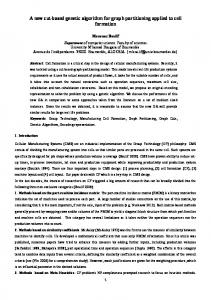
One possible explanation of the success of the no-shuffling strategy is illustrated in Figure 4. Solutions that are far

6

Graph add20 data 3elt uk add32 bcsstk33 whitaker3 crack wing nodal fe 4elt2 vibrobox bcsstk29 4elt fe sphere cti memplus cs4

Number of vertices 2395 2851 4720 4824 4960 8738 9800 10240 10937 11143 12328 13992 15606 16386 16840 17758 22499

Number of edges 7462 15093 13722 6837 9462 291583 28989 30380 75488 32818 165250 302748 45878 49152 48232 54196 43858

Graph bcsstk30 bcsstk31 fe pwt bcsstk32 fe body t60k wing brack2 finan512 fe tooth fe rotor 598a fe ocean 144 wave m14b auto

Number of vertices 28924 35588 36519 44609 45087 60005 62032 62631 74752 78136 99617 110971 143437 144649 156317 214765 448695

Number of edges 1007284 572914 144794 985046 163734 89440 121544 366559 261120 452591 662431 741934 409593 1074393 1059331 1679018 3314611

TABLE II I NSTANCES IN WALSHAW ’ S G RAPH PARTITIONING A RCHIVE

G500.2.5 G500.05 G500.10 G500.20 G100.2.5 G1000.05 G1000.10 G1000.20 U500.05 U500.10 U500.20 U500.40 U1000.05 U1000.10 U1000.20 U1000.40 Population

Without shuffling Average Min 49.1 49 218 218 626.7 626 1744 1744 94.55 93 447.35 445 1362.65 1362 3383.5 3382 2 2 26 26 178.1 178 412 412 1.2 1 39.05 39 222 222 737 737 = 200, STUCK = 100, 20 runs per instance

Iter 157.1 117.6 129.55 124 188.45 202.25 174.9 161.45 122.6 104.3 102.55 102 131.1 111.3 104.25 102.25

Average 52.25 219.4 630.2 1749.8 99.45 452.8 1366.15 3387.4 2.1 26 178.25 412 1 39 222 737

With shuffling Min 51 218 627 1744 96 450 1363 3385 2 26 178 412 1 39 222 737

Iter 109.75 113.4 108.95 110.6 115.5 117.2 117.55 118.7 105.8 103.4 102.35 102 106.1 106.4 103.7 102.1

Best known 49 218 626 1744 93 445 1362 3382 2 26 178 412 1 39 222 737

TABLE III C OMPARISON OF PERFORMANCES OF POPULATION PRODUCTION STRATEGIES

apart in the population evolve independently for a number of generations (provided the solutions in the starting population are produced independently.) More precisely, for a population of P solutions indexed from 0 to P − 1 we define the distance between solution of index i and solution of index j as the length of the shortest path between i and j in the cycle 0, 1, 2 . . . P − 1, 0. This distance is min(|i − j|, P − |i − j|). Two solutions at distance d evolve independently for d − 1 generations, as illustrated by the two triangles highlighted in Figure 4. In Figure 4 solution of index 0 and solution of index 5 are at distance 4 in a population of size 9 and evolve independently for 3 generations. This indicates that a diverse population may be maintained for longer when using a no-shuffling strategy. As a consequence runs with the no-shuffling strategy may require more iterations than runs with the shuffling strategy but may also converge to better solutions. This seems to be confirmed by the results in Table III, as the number of iterations for the no-shuffling

strategy is always higher than the number of iterations for the shuffling strategy, and the average and minimum cut values obtained for the harder Gn.d instances are always better. For the Un.d instances that are easy to solve there is not a huge difference between strategies as the best cut value is found early on by both methods. However for the three most difficult instances to solve, which are G500.2.5, G100.2.5 and G1000.05 (see Table V in Section V-E), the effect is more pronounced. B. Convergence of The Algorithm In Section III-A we showed that PROBE converges to a population of solutions with identical values when an exact method is used to generate child solutions. We shall call the value to which solution values converge the convergence value. In our practical implementation children solutions are generated from parent solutions heuristically. Nonetheless convergence also happens as shown by experiments illustrated

7

U500.05

G500.2.5

50

110 100

40

90 80

30

70

20

60

10

50 40 1

50

100

150

200

250

300

350

400

450

0 1

50

100

150

200

250

G500.10

300

350

400

450

500

550

U1000.05 680

30

670

25

660

20

650

15

640

10

630

5

620 1

150

300

450

600

750

900

1050

1200

0 1

250

500

G1000.2.5

750

1000

1250

U1000.10 120

120 110 100 90 80 70 60 50 40 30

115 110 105 100 95 90 1

100

200

300

400

500

600

700

800

900

1000 1100

Fig. 5. Maximum, average, and minimum solution values over the population versus generation number for Gn.d graphs

in Figures 5 and 6 for a sample of the graphs. See the Appendix for a complete set of figures for all Gn.d and Un.d graphs. These figures correspond to experiments with a population of 50 solutions. They provide graphs of the maximum, average, and minimum solution values over the population at every five generations. Each experiments is terminated when the three values are identical for twenty five consecutive generations. The minimum cut value found in an experiment is usually found rapidly, the average solution value tends to decrease smoothly, while diversity in the population is maintained for a large number of iterations as shown by the more erratic behavior of the maximum value. The convergence to a population where all solutions have identical values is a striking feature of our experiments. Observe that sometimes the minimum value increases. There is no reason this should not happen as a good solution may be lost from one generation to the next. In general the convergence value is close to the optimum value, but it is by no means always the case. The graph for U1000.10 is a particularly interesting “bad case”.

1

50

100

150

200

250

300

350

400

450

500

Fig. 6. Maximum, average, and minimum solution values over the population versus generation number for Un.d graphs

The minimum value of 39 is found at generation 31 (this is the best know solution value for this instance.) The minimum value then oscillates between 39 and 40 until generation 456 when it becomes 52 after which both maximum, average, and minimum values converge rapidly to 52. An identical behaviour is observed if we increase the population to 200. In this case the value 39 is obtained at generation 16. The same oscillations of the minimum value between 39 and 40 are observed until generation 456 when the minimum becomes 51 and remains so until convergence. Obviously, this does not affect the effectiveness of our method as we tend to find the minimum cut value before convergence occurs. The graph for instance G1000.2.5 is also interesting. The minimum value of 95 is found at generation 136 and remains so for 584 generations until an improved value of 94 is found. The convergence value is 94 in this experiment. In practice we do not wait for convergence to terminate a run of our algorithm. Instead we stop when no improvement of the minimum value

8

has occurred for a number of iterations (parameter STUCK.) We use a relatively small value of the parameter STUCK in our experiments in order to limit computing time. This can however be at the detriment of the quality of the final solution for some runs as indicated by the above observation.

average value / best known value

C. Influence of The Population Size 1.05 1.04 30

1.03

50 100

1.02

150

1.01

200

1 0.99

average value / best known value

G500.2.5

G500.05

G500.10

G500.20

G100.2.5

G1000.05

G1000.10

G1000.20

1.1 1.09 1.08 1.07

30

1.06 1.05

50 100

1.04 1.03

150 200

1.02 1.01 1 0.99 U500.10

U500.20

U500.40

U1000.10

U1000.20

U1000.40

average value / best known value

4.5

the minimum, maximum, average of this output and average CPU time of a multi-run over 5 multi-runs of the algorithm. The computational time of a run with a population of size kP may be assumed to be roughly k times the computational time of a run with a population of size P . This assumption is not entirely correct as the algorithm does not stop after a fixed number of generations but when the minimum value has not been improved for a number of consecutive generations. However, the assumption seems to be reasonable without any prior knowledge for an input instance. So as we divide the population by 2 we multiply r by 2. The average times of multi-runs displayed in the table confirm our assumption. The results in Table IV indicate that to perform a small number of runs with a large population is a slightly better strategy than performing a large number of runs with a small population both in terms of minimum cut value and maximum cut value. It should also be noted that our current implementation is not particularly memory-consuming. Each individual in the population is represented in compact form as a bit string. We also keep the difference values (see Section IV-B) of the vertices in the corresponding bisection. These difference values are exploited to avoid initialization from scratch of the bucket array structure when the Differential-Greedy algorithm is applied (see Section IV-A.) So as our implementation stands the memory complexity associated with the population is O(nP ).

4 3.5

30

3

50

2.5

100

2

150 200

1.5 1 0.5 U500.05

U1000.05

Fig. 7. Influence of population size on quality of solutions, 20 runs per size

In Figure 7 we display the quality of the average cut value found over 20 runs for various population sizes. In these experiments the value of the parameter STUCK is 50 (we stop the method after 50 generations without improvement of the minimum cut value found.) For normalization purposes the average cut value is divided by the best known cut value shown in the last column of Table III. As the population increases the average cut value decreases. To get solution values consistently close to the optimum cut value a population of at least 50 solutions should be used. Note that the optimum cut value for U1000.05 is 1 which explains the greater ratios observed. For this instance a ratio of 1.5 indicates that the optimal cut value is found in at least 50% of the runs. D. Many Short Runs or a Small Number of Long Runs? Should we perform a small number of runs with a large population of solutions or a large number of runs with a small population of solutions? We address this question in this section. A multi-run is produced by performing a number r of runs of the algorithm. The output of a multi-run is the best cut value found in the r runs of the algorithm. In Table IV we give

E. Performance Quality In Table V, Table VI and Table VII we compare the performance of our algorithm with results obtained with Bui and Moon’s GA [19], Battiti and Bertossi’s RRTS [18] (see Sections II for a brief presentation of these algorithms) and Saab’s partitioning method TPART [26]. According to Bui and Moon’s results their algorithm dominates the simulated annealing algorithm presented in [15] as well as a multi-start Kernighan and Lin algorithm. For each method we provide, whenever available, the average, standard deviation, minimum and maximum cut values over a number of runs for each instance considered. We ran PROBE BA with a population of 200 solutions, and a value of 100 for the parameter STUCK; and performed 40 runs with different random initializations for each graph. Results in the column “TPART(5) 100 runs” correspond to 100 runs of the method TPART with 5n moves in its main algorithm, and are those published in [26]. Results reported for the other techniques correspond to 1000 runs per instance. Results in columns “BFS GBA 1000 runs” are those published in [19]. Results in columns “RRTS 1000 runs” are those published in [18]. The best results are displayed in boldface. All CPU times are average CPU times of a single run. The minimum values returned by PROBE BA for the Gn.d and Un.d graphs are the best known values for these instances. In fact, for G1000.2.5 we improve on the best value found by the other methods. The computing time of a run with PROBE is much larger than with the other methods. However, the method delivers quality results. All runs of PROBE BA

9

Population=200, r=4 Min Max Ave CPU Min G500.2.5 49 49 49 14.2 49 G500.05 218 218 218 13.6 218 G500.10 626 627 626.2 19.9 626 G500.20 1744 1744 1744 30.5 1744 G100.2.5 93 94 93.8 34.4 94 G1000.05 445 446 445.2 46.7 445 G1000.10 1362 1362 1362 54.0 1362 G1000.20 3382 3384 3382.8 77.6 3383 U500.05 2 2 2 12.3 2 U500.10 26 26 26 12.1 26 U500.20 178 178 178 19.5 178 U500.40 412 412 412 25.5 412 U1000.05 1 1 1 25.7 1 U1000.10 39 39 39 28.0 39 U1000.20 222 222 222 45.8 222 U1000.40 737 737 737 57.7 737 min, max, average cut and cpu over 5 multi-runs per instance r = number of runs in a multi-run; STUCK = 100

Population=100, r=8 Max Ave 49 49 218 218 627 626.6 1744 1744 95 94.2 448 446 1362 1362 3384 3383.4 2 2 26 26 178 178 412 412 1 1 39 39 222 222 737 737

CPU 15.0 15.0 22.5 32.3 37.3 43.2 60.7 82.2 12.3 12.2 20.0 25.6 30.2 31.8 52.6 60.8

Min 49 218 626 1744 94 445 1362 3382 2 26 178 412 1 39 222 737

Population=50, r=16 Max Ave 49 49 218 218 627 626.6 1744 1744 94 94 448 446.2 1362 1362 3384 3382.8 2 2 26 26 178 178 412 412 1 1 39 39 222 222 737 737

CPU 15.2 16.2 22.6 34.2 38.0 46.0 64.8 87.9 12.3 12.7 20.3 25.9 30.8 33.7 46.9 61.6

TABLE IV C OMPARISON OF RUN STRATEGIES

BFS GBA 1000 runs Graph G500.2.5 G500.05 G500.10 G500.20 G1000.2.5 G1000.05 G1000.10 G1000.20

Ave 53.97 222.13 631.46 1752.51 103.61 458.55 1376.37 3401.74

Min 49 218 626 1744 95 447 1362 3382 TPART(5) 100 runs

RRTS 1000 runs (1000n iterations per run) CPU1 0.029 0.040 0.058 0.106 0.083 0.117 0.183 0.307

Graph Ave Min CPU1 G500.2.5 53.21 50 0.032 G500.05 223.42 218 0.072 G500.10 631.44 626 0.133 G500.20 1751.88 1744 0.289 G1000.2.5 99.64 94 0.089 G1000.05 459.69 448 0.200 G1000.10 1372.76 1363 0.400 G1000.20 3403.28 3382 0.728 1: Original CPU time normalized to discount the different speed of †: MAXITER = 200, STUCK = 100

Ave 52.06 218.29 626.44 1744.36 98.69 450.99 1364.27 3383.92 Ave 49.12 218 626.85 1744.07 94.62 447.5 1362.4 3383.52 the machines

St.dev. 0.50 0.46 0.59 0.66 1.01 1.43 1.38 1.00 PROBE BA 40 runs† St.dev. 0.33 0.00 0.36 0.47 0.70 1.30 0.59 0.82

Min 49 218 626 1744 93 445 1362 3382

Min 51 218 626 1744 95 445 1362 3382 Max 50 218 627 1747 96 450 1364 3385

CPU1 0.125 0.156 0.225 0.425 0.406 0.406 0.581 0.919 CPU 3.59 3.54 4.90 7.51 8.86 12.0 14.3 21.2

TABLE V C OMPARISONS BETWEEN SOLUTION METHODS

provide solutions close to the best found, except for instance U1000.05. For this instance we found the optimal cut value 1 in 32 of the runs and values greater than 2 in only 4 runs. The worst cut values found by our method are in all cases but one better than the average cut values obtained with BFS GBA. Our average cut value is also most of the time less than or equal to that of RRTS but RRTS gives good quality results in shorter computing time. More importantly, for the difficult instances, we obtained better results than RRTS. For instance G500.2.5 our maximum cut value is less than the minimum cut value obtained by RRTS in 1000 runs. In fact in 40 runs we got cut values of 49 (35 times) and 50 (5 times). For instance G1000.2.5, the best cut value found by BFS GA and RRTS

in 1000 runs is 95. PROBE BA obtained cut values of 93 (1 time), 94 (10 times), 95 (21 times), 96 (8 times). TPART finds good cut values but sometimes fails to find the minimum cut value. The average values also indicate that the method is not as consistent as PROBE BA. However the computing times are very low. So the consistency (average cut value) can be improved by using a multi-run strategy (see [26] for details.) For the breg.n.b, grid.n.b and w-grid.n.b instances our algorithm performs well in terms of quality. These instances are however also well solved by the much faster methods, BFS GBA and TPART. For the caterpillar graphs our algorithm has difficulties in finding good solutions when the graph size increases. This may be because we use a version of KL

10

BFS GBA 1000 runs Graph U500.05 U500.10 U500.20 U500.40 U1000.05 U1000.10 U1000.20 U1000.40

Ave 3.65 32.68 179.58 412.23 1.78 55.78 231.62 738.10

Min 2 26 178 412 1 39 222 737 TPART(5) 100 runs

RRTS 1000 runs (1000n iterations per run) CPU1 0.037 0.047 0.057 0.049 0.087 0.152 0.162 0.182

Ave 2 26 178 412 1 39.03 222 737

Graph Ave Min CPU1 Ave U500.05 2.34 2 0.024 2.05 U500.10 28.35 26 0.061 26 U500.20 179.05 178 0.161 178 U500.40 412 412 0.261 412 U1000.05 1.06 1 0.043 1.4 U1000.10 42.71 39 0.150 39 U1000.20 227.88 222 0.333 222 U1000.40 745.34 737 0.750 737 1: Original CPU time normalized to discount the different speed of the machines †: MAXITER = 200, STUCK = 100

St.dev. Min 0 2 0 26 0 178 0 412 0 1 0.19 39 0 222 0 737 PROBE BA 40 runs† St.dev. 0.22 0 0 0 0.96 0 0 0

Min 2 26 178 412 1 39 222 737

CPU1 0.106 0.169 0.331 0.638 0.263 0.394 0.781 1.519 Max 3 26 178 412 5 39 222 737

CPU 3.17 3.11 5.10 6.79 6.98 7.41 11.7 15.3

TABLE VI C OMPARISONS BETWEEN SOLUTION METHODS

BFS GBA 1000 runs

TPART(5) 100 runs

Graph Ave Min CPU1 Ave Min breg500.0 0 0 0.011 0 0 breg500.12 12 12 0.019 12 12 breg500.16 16 16 0.020 16.02 16 breg500.20 20 20 0.021 20.10 20 breg5000.0 0 0 0.198 0 0 breg5000.4 4 4 0.212 4 4 breg5000.8 8 8 0.221 8 8 breg5000.16 16 16 0.260 16 16 cat.352 2.25 1 0.011 1 1 cat.702 2.43 1 0.031 1 1 cat.1052 2.44 1 0.049 1 1 cat.5252 2.63 1 0.329 1 1 rcat.134 1.35 1 0.003 1 1 rcat.554 1.99 1 0.015 1 1 rcat.994 2.14 1 0.031 1 1 rcat.5114 2.36 1 0.259 1 1 gridl00.10 10 10 0.002 10 10 grid500.21 21.02 21 0.017 21 21 grid1000.20 20 20 0.037 20 20 grid5000.50 50 50 0.301 50 50 w-grid100.20 20 20 0.003 20 20 w-grid500.42 42 42 0.023 42 42 w-grid1000.40 40 40 0.052 40 40 w-grid5000.100 100.03 100 0.464 100 100 1: Original CPU time normalized to discount the different speed of the machines †: MAXITER = 200, STUCK = 100

PROBE BA 40 runs† CPU1 0.002 0.021 0.022 0.024 0.024 0.244 0.244 0.272 0.007 0.013 0.021 0.100 0.003 0.010 0.017 0.089 0.005 0.026 0.054 0.328 0.006 0.029 0.056 0.350

Ave 0 12 16 20 0 4 8 16 1 2.55 2.4 8.65 1 1.15 1.25 2.57 10 21 20 50 20 42 40 100

Min 0 12 16 20 0 4 8 16 1 1 1 5 1 1 1 2 10 21 20 50 20 42 40 100

CPU 0.610 1.12 1.09 1.09 9.60 14.6 14.9 14.3 0.85 1.69 3.26 24.1 0.27 1.23 2.42 19.9 0.27 1.1 2.27 14.0 0.296 1.23 2.40 15.2

TABLE VII C OMPARISONS BETWEEN SOLUTION METHODS

in our improvement phase; KL is known to perform poorly for caterpillar graphs [34]. We use the same version of KL as BFS GA but the breadth first search preprocessing of BFS GA is the main factor in the success of the GA for these instances. Without the preprocessing the best cut values found by Bui and

Moon’s GA for identical experiments is 69 for cat.5252 and 11 for rcat.5114 (see [19].) TPART is the best of the methods tested for solving caterpillar graphs. The benefit of multilevel methods that may coarsen the graph by collapsing the legs of the caterpillar is clear.

11

RRTS (100n iterations per run) Graph airfoil1 big wave bcspwr09 bcsstk13 nasa4704 DEBR12 DEBR18 Graph airfoil1 big wave bcspwr09 bcsstk13 nasa4704 DEBR12 DEBR18

Ave 74.8 141.3 8950.8 9.3 2355 1296.0 558.0 24088.8 TPART(5,20) Ave 74 139 8727.2 9 2355 1292 548 23486

Min 74 139 8704 9 2355 1292 548 23208

St.dev. 1.1 2.2 74.7 0.6 0 7.0 1.7 114.2 CPU1 9.3 40.9 4508 1.2 34.3 54.6 13.5 6533

Min 74 139 8835 9 2355 1292 556 23996 PROBE BA, Population=50†

Ave St.dev. 74 0 157.6 17.38 8717.8 10.31 9 0 2355 0 1292 0 548 0 23651 246.57 PROBE BA, population=200†

Min 74 139 8701 9 2355 1292 548 23442

Graph Ave St.dev. Min airfoil1 74 0 74 big 141.2 5.9 139 wave 8709.1 4.3 8702 bcspwr09 9 0 9 bcsstk13 2355 0 2355 nasa4704 1292 0 1292 DEBR12 548 0 548 DEBR18 23438.2 32.8 23352 1: Original CPU time normalized to discount the different speed of the machines †: MAXITER = 250, STUCK = 100

CPU1 0.41 2.1 288 0.12 0.73 1.2 0.91 3537

Max 74 187 8737 9 2355 1292 548 24226

Max 74 158 8715 9 2355 1292 548 23470

CPU 8.6 42.8 1480 3.0 11.0 12.7 9.14 2340 CPU 30.9 164 5729 11.7 41.3 51.1 32.7 9804

TABLE VIII C OMPARISONS ON “ PARALLEL COMPUTING ” GRAPHS OVER 10 RUNS FOR EACH METHOD

Table VIII compares PROBE BA, RRTS, and Saab’s multilevel algorithm TPART(5,20) (each run is the best of 20 runs of TPART(5)) over 10 runs of each method on the graphs of Table I. All CPU times are average CPU times of a single run. The results for RRTS are those published in [18]. The results for TPART are those published in [26]. The results of Battiti and Bertossi also showed that RRTS gives at least as good or better cut values than state-of-the-art partitioning software MeTis, Chaco, Scotch and Party for the instances tested excepted for DEBR12 where Party with Helpful Sets found a minimum cut value of 548 (see [18] for details.) Best results are shown in boldface in the table. PROBE BA was run with populations of 50 and 200 solutions with, in each case, a maximum number of iterations of 250, and the parameter STUCK set to 100. PROBE BA always find as good or better minimum cut values than RRTS. For instances wave and DEBR12 the worst result (column Max) of PROBE BA for both population sizes is better than the best result (column Min) found by RRTS. This also applies to DEBR18 when PROBE BA is run with a population of 200 solutions. There is not much difference in terms of quality of solutions between TPART and PROBE BA; both methods find good solutions and produce low average cuts in similar computing time (after re-scaling). TPART finds a better cut value than PROBE BA

with population 200 for DEBR18 but for both DEBR18 and wave the maximum cut value found by PROBE BA is lower than the average cut value found by TPART, which indicates a greater consistency in the quality of results with PROBE BA for these instances. PROBE BA with both population 50 and 200 finds a better cut value than TPART for wave. Note also that in the experiments of Section V-F below we report a cut value of 8692 edges for this instance. Saab points out that it is possible to obtain high quality solutions with his method much faster. He mentions that he obtained a cut value of 23650 edges for DEBR18 in 116.7 seconds (equivalent to 64.8 seconds on our machine) by running TPART(1,1). However he does not provide information that would indicates whether this is a typical run or the best run amongst many. The latter hypothesis seems more likely given the results of TPART(1,1) on smaller graphs. By running PROBE BA with a population of 50, and the parameter STUCK set to 5 (we stop as soon the minimum cut value does not steadily decrease) we obtained the following results for the more difficult instances: PROBE BA 10 runs, population=50† Graph Ave St.dev. wave 8858.8 49.8 DEBR18 24049.8 286.5 †: MAXITER = 100, STUCK = 5

Min 8823 23698

Max 8967 24572

CPU 256 810

12

Graph add20 data 3elt uk add32 bcsstk33 whitaker3 crack wing nodal fe 4elt2 vibrobox bcsstk29 4elt fe sphere cti memplus cs4

Best 599 190 90 20 11 10171 127 184 1707 130 10343 2843 139 386 334 5538 372

Min 596 189 90 20 11 10171 127 184 1707 130 10343 2843 139 386 334 5513 372

Ave. 598.25 190.8 90 25.4 12.9 10171 127.1 184.05 1708.05 130 10343 2843 140.9 386 334 5576.85 402.6

Graph Best Min bcsstk30 6394 6394 bcsstk31 2768 2762 340 340 fe pwt bcsstk32 4667 4667 fe body 262 266 t60k 80 423 wing 791 809 brack2 731 731 finan512 162 162 3850 3897 fe tooth fe rotor 2103 2098 598a 2411 2398 465 464 fe ocean 144 6491 6490 wave 8704 8692 m14b 3836 3837 auto 10173 10117 †: Population = 100, MAXITER = 200, STUCK = 100 ‡: Population = 50, MAXITER = 200, STUCK = 100

Ave. 6394 2827.6 340.4 5122.8 342.1 531.4 998.6 731 226.8 3977.1 2099.1 2400 473.7 6497.9 8707.1 3841.8 10198.7

PROBE BA, 20 runs† St.dev. 0.97 2.63 0 3.27 3.02 0 0.31 0.22 1.54 0 0 0 4.39 0 0 56.63 40.67 PROBE BA, 10 runs‡ St.dev. 0 197.33 0.84 469.29 76.21 75.38 107.96 0 83.65 86.61 1.28 1.49 8.47 6.70 6.43 2.25 59.48

Max 600 198 90 32 20 10171 128 185 1713 130 10343 2843 158 386 334 5689 548

CPU 8.8 16.6 18.2 24.1 23.0 123.5 32.1 51.1 111.3 41.8 119.6 93.7 89.6 79.4 55.5 120.0 199.1

Max 6394 3389 342 5811 467 662 1118 731 324 4102 2101 2402 495 6510 8714 3845 10304

CPU 198.4 201.5 104.9 337.4 186.4 181.2 370.4 188.8 211.0 332.8 567.0 808.4 589.7 1871 1239 2117 5908

TABLE IX P ERFORMANCE OF PROBE BA ON WALSHAW ’ S G RAPH PARTITIONING A RCHIVE INSTANCES

This shows that our method finds good quality solutions rapidly. The relative gap between the average cut values shown above and the best cut values displayed in Table VIII is 1.8% (3.6%) for wave (DEBR18). The minimum cut values are also better than those found by RRTS in Table VIII. F. Solution of the Walshaw Graph Partitioning Archive instances Table IX gives results for the instances in Walshaw’s Graph Partitioning Archive. For the smaller instances we performed 20 runs with a population of 100 solutions whereas for the larger instances we performed 10 runs with a population of 50 solutions. In both cases we limited the number of generations to 200. For each graph we give the minimum, average, standard deviation, and maximum of the best cut value found over the number of runs performed. CPU is the computing time for one run. Column “Best” is the best known solution value. Best known cut values have been obtained by various researchers using approaches ranging from KL based

partitioning techniques to semi-definite programming (see the archive for details.) PROBE BA does not find the best known cut value for 5 instances. It seems that our algorithm does not work well with instance t60k. t60k is a 2D Finite Element Method dual graph where the maximum vertex degree is 3 and the minimum vertex degree is 1 Other instances in the archive are also dual graphs (e.g. uk, cs4, wing.) PROBE BA find the best cut value previously reported for 19 instances, and an improved cut value for 10 instances. Note that the results for wave in this group of experiments are slightly better than those reported in Table VIII (the difference in CPU per run is due to a different choice of the MAXITER parameter.) PROBE BA’s consistency varies according to the instances, as shown by the maximum cut values and the standard deviations. The population used for the larger instances was however relatively small. For fe rotor and 598a all 10 runs provide an improvement on the previously best known

13

cut value. VI. C ONCLUSION The main objective of our research was to test the recently proposed metaheuristic PROBE on an important combinatorial optimization problem. PROBE BA, our specialization of PROBE for the solution of the GBP, enabled us to establish a number of interesting properties that would be worth investigating further with other combinatorial optimization problems: The impact of the population is significant as runs with large population sizes give better solutions than runs with small population sizes. The strict ordering of solutions which maintains a degree of independence between solutions for a number of generations, is an important factor in the success of the method. Populations seem to converge to solutions of identical objective values even when there is no enforced requirement that a solution should have a better fitness than its parent solutions. Importantly, we showed that PROBE BA can compete with other algorithms based on Genetic Algorithms, Reactive Tabu Search, or more specialized multilevel partitioning techniques. PROBE BA also finds improved best cut values on a number of real world instances. PROBE BA uses standard graph partitioning methods to explore search spaces and perform local optimization, namely the Differential-Greedy algorithm of Battiti and Bertossi and a modification of KL due to Bui and Moon. It would be interesting to investigate whether PROBE can enhance the power of other graph partitioning algorithms. Another interesting line of investigation would be to develop a PROBE-based algorithm for the solution of k-way partitioning problems. In this case several bits per vertex could be used to code the indices of the partitions to which vertices are assigned. The search of a subspace would require a partitioning algorithm that can construct as good a solution as possible from a partially initialized solution (i.e., vertices pre-assigned to partitions.) A PPENDIX I The set of convergence graphs mentioned in Section V-B is provided for the Gn.d and Un.d instances.

14

G500.2.5

G500.05 110

280

100

270

90

260

80

250

70

240

60

230

50

220

40 1

50

100

150

200

250

300

350

400

210 1

450

50

100

150

200

250

300

G500.10

350

400

450

500

550

600

G500.20 1820

680

1810

670

1800

660

1790

650

1780 1770

640

1760

630

1750

620 1

150

300

450

600

750

900

1050

1740

1200

1

20

40

60

80

100

120

140

160

180

200

220

G1000.05

G1000.2.5 120

520 510

115

500

110

490

105

480

100

470 460

95

450

90 1

100

200

300

400

500

600

700

800

900

1000

1100

440 1

100

200

300

400

G1000.10

500

600

700

800

900

1000

G1000.20 1400

3520

1395

3500

1390 1385

3480

1380

3460

1375

3440

1370

3420

1365

3400 3380

1360 1

Fig. 8.

100

200

300

400

500

600

700

800

900

1

150

300

450

600

750

900

Maximum, average, and minimum solution values over the population versus generation number for Gn.d graphs

1050 1200 1350

1500

15

U500.10

U500.05

85

50

75

40

65

30

55

20

45

10 0 1

50

100

150

200

250

300

350

400

450

500

550

35 25 1

50

100

150

290

1580

270

1380

250

1180

230

980

210

780

190

580 380

170 100

200

300

400

500

600

250

U500.40

U500.20

1

200

700

800

1

900

5

10

15

U1000.05

20

25

30

35

U1000.10 120 110 100 90 80 70 60 50 40 30

30 25 20 15 10 5 0 1

250

500

750

1000

1

1250

50

100

150

200

250

300

350

400

450

U1000.40

U1000.20

510

1420

460

1320 1220

410

1120

360

1020

310

920

260

820

210 1

Fig. 9.

50

100

150

200

500

250

300

720 1

5

10

15

Maximum, average, and minimum solution values over the population versus generation number for Un.d graphs

20

25

30

16

R EFERENCES [1] Bui, T.N. and Jones, C., “A Heuristic for Reducing Fill in Sparse Matrix Factorization,” in Proc. Sixth SIAM Conf. Parallel Processing for Scientific Computing, 1993, pp. 445–452. [2] Alpert, C. and Kahng, A., “Recent Directions in Netlist Partitioning: A Survey,” Integration-The VLSI J., vol. 19, no. 1-2, pp. 1–81, 1995. [3] Johannes, F.M., “Partitioning of VLSI Circuits and Systems,” in Proc. Design Automation Conf., 1996, pp. 83–87. [4] Fox, G.C., “A Review of Automatic Load Balancing an Decomposition Methods for the Hypercube,” in Numerical Algorithms for Modern Parallel Computer Architectures, Schultz, M., Ed. Springer-Verlag, 1988, pp. 63–76. [5] Sanchis, L., “Multiple-Way Network Partitioning,” IEEE Transactions on Computers, vol. 38, pp. 62–81, 1989. [6] Simon, H.D., “Partitioning of Unstructured Problems for Parallel Processing,” Computing Systems in Eng., vol. 2, pp. 135–148, 1991. [7] Gilbert, J.R. and Miller, G. L. and Temg, S.H., “Geometric Mesh Partitioning: Implementation and Experiments,” in Proc. Internationall Parallel Processing Symp. (IPPS’95), 1995. [8] Hendrickson, B. and Leland, R., “An Improved Spectral Graph Partitioning Algorithm for Mapping Parallel Computations,” SIAM J. Scientific Computing, vol. 16, no. 2, pp. 452–469, 1995. [9] Ding, C. and Xiaofeng, H. and Hongyuan, Z. and Ming, G. and Simon A., “Min-Max Cut Algorithm for Graph Partitioning and Data Clustering,” in Proc. IEEE International Conf. Data Mining, 2001, pp. 107–114. [10] Dunlop, A. and Kernighan, B., “A Procedure for Placement of StandardCell VLSI Circuits,” IEEE Trans. Computer-Aided Design of Integrated Circuits and Systems, vol. 1, pp. 92–98, 1985. [11] Barahona, F. and Gr¨otchel, M. and J¨unger, M. and Reinelt, G., “Application of Combinatorial Optimization to Statistical Physics and Circuit Layout Design,” Operations Research, vol. 36, pp. 493–513, 1988. [12] Kernighan, B.W. and Lin, S., “An Efficient Heuristic Procedure for Partition Graphs,” Bell Systems Technical J., vol. 49, pp. 291–307, February 1970. [13] Fiduccia, C. and Mattheyses, R., “A Linear Time Heuristics for Improving Network Partitions,” in Proc. 29th ACM/IEEE Design Automation Conf., 1982, pp. 175–181. [14] Garey, M. D. and Johnson, D. S. and Stockmeyer, L., “Some Simplified NP-Complete Graph Problems,” Theoretical Computer Science, vol. 1, pp. 237–267, 1976. [15] Johnson, D.S. and Aragon, C.R. and McGeoch, L.A. and Schevon, C., “Optimization by Simulated Annealing: An Experimental Evaluation; Part I, Graph Partitioning,” Operations Research, vol. 37, pp. 865–892, 1989. [16] Dell’Amico, M. and Maffioli, F., “A New Tabu Search Approach to the 0-1 Equicut Problem,” in Meta-Heuristics 1995: The State of the Art. Kluwer Academic, 1996, pp. 361–377. [17] Rolland, E. and Pirkul, H. and Glover, F. , “Tabu Search for Graph Partitioning,” Annals of Operational Research, vol. 63, pp. 209–232, 1996. [18] Battiti, R. and Bertossi, A., “Greedy, Prohibition and Reactive Heuristics for Graph Partitioning,” IEEE Transactions on Computers, vol. 48, pp. 361–385, 1999. [19] Bui, T.N. and Moon, B.R., “Genetic Algorithm and Graph Partitioning,” IEEE Transactions on Computers, vol. 45, pp. 841–855, 1996. [20] Steenbeek, A.G. and Marchiori, E. and Eiben, A. E., “Finding Balanced Graph Bipartitions Using a Hybrid Genetic Algorithm,” in Proc. of the IEEE International Conf. on Evolutionary Computation ICEC’98, 1998, pp. 90–95. [21] Laguna, M. and Feo, T.A. and Elrold, H.C., “Adaptive Search Procedure for the Two-Partition Problem,” Operations Research, vol. 42, pp. 677– 687, 1994. [22] Barnard, S.T. and Simon, H.D., “Fast Multilevel Implementation of Recursive Spectral Bisection for Partitioning Unstructured Problems,” Concurrency: Practice and Experience, vol. 6, no. 2, pp. 101–117, 1994. [23] Karypis, G. and Aggarwal, R. and Kumar, V. and Shekhar, S., “Multilevel Hypergraph Partitioning: Application in VLSI Domain,” in Proc. of Design Automation Conf., 1997, pp. 526–529. [24] Alpert, C.J. and Huang, J.-H. and Kahng, A.B. , “Multilevel Circuit Partitioning,” in Proc. Design Automation Conf., 1997, pp. 530–533. [25] Saab, Y.G., “A New 2-Way Multi-Level Partitioning Algorithm,” VLSI Design J., vol. 11, no. 3, pp. 301–310, 2000. [26] Saab,Y.G., “An Effective Multilevel Algorithm for Bisecting Graphs and Hypergraphs,” IEEE Transactions on Computers, vol. 53, no. 641-652, 2004.

[27] Walshaw, Chris, “Multilevel Refinement for Combinatorial Optimisation Problems,” Annals of Operations Research, no. 131, p. 325372, 2004. [28] Battiti, R. and Bertossi, A., “Differential Greedy for the 0-1 Equicut Problem,” in Proc. of the DIMACS workshop on Network Design; Connectivity and Facilities Location, Du, D.Z. and Pardalos, P.M., Ed. AMS, 1997. [29] Barake, M. Chardaire, P. and McKeown, G. P., “The PROBE Metaheuristic for the Multiconstraint Knapsack Problem,” in Metaheuritics, Resende, M. G. C. and de Sousa, J. P., Ed. Springer, 2004, pp. 19–36. [30] Zbigniew Michalwicz, Genetic Algorithms + Data Structures = Evolution Programs. Springer, 1996. [31] Bui, T.N. and Chaudhuri, S. and Leighton, F.T. and Sipser, M., “Graph Bisection Algorithms with Good Average Case Behavior,” Combinatorica, vol. 7, no. 2, pp. 171–191, 1987. [32] Duff, I.S. and Grimes, R.G. and Lewis, J.G., “Sparse Matrix Test Problems,” ACM Trans. Math. Software, vol. 15, no. 1, pp. 1–14, 1989. [33] Soper, A. J. and Walshaw, C. and Cross, M., “A Combined Evolutionary Search and Multilevel Optimisation Approach to Graph Partitioning,” Journal of Global Optimization, vol. 29, no. 2, pp. 225–241, 2004. [34] Jones, C., “Vertex and Edge Partitions of Graphs,” Ph.D. dissertation, Pennsylvania State University, Pa., 1992.

Pierre Chardaire Biography text here.

PLACE PHOTO HERE

Musbah Barake Biography text here.

PLACE PHOTO HERE

Geoff P. McKeown Biography text here.

PLACE PHOTO HERE