A Robust One-Class Support Vector Machine Using Gaussian ... - ijmmm

International Journal of Materials, Mechanics and Manufacturing, Vol. 5, No. 3, August 2017

A Robust One-Class Support Vector Machine Using Gaussian-Based Penalty Factor and Its Application to Fault Detection T. Prayoonpitak and S. Wongsa  Abstract—In recent years, one-class support vector machine (SVM) approaches have received particular attention in fault detection since only one class of the data is required for training. However, the training data can be corrupted with the outliers that influence classifier performance significantly. In this paper, a Gaussian-based penalisation has been proposed in the formation of a robust one-class SVM model which constructs the decision boundaries that are robust to the outliers without compromising the classification performance. The efficacy of the proposed method has been compared with the traditional one-class SVM and a previous robust one-class SVM method in the literature when applied in three datasets: the Iris’s Fisher dataset, banana-shaped dataset and MFPT bearing fault dataset. It is shown that the proposed robust one-class SVM outperforms other methods. Index Terms—Robust one-class SVM, penalty factor, fault detection, outliers.

I. INTRODUCTION Novelty detection is the task of classifying test data that differ in some respect from the data that are available during training. This may be referred as “one-class classification”, in which a model is constructed to describe a dataset when only one class of dataset is available. The model is then used to detect whether a new sample resembles the training dataset according to the constructed description. Many methods have been proposed to solve one-class classification problems in recent years. Among all the method available for one-class classification problems, Support vector machine (SVM) is one of the most famous and popular techniques which has been applied for fault detection in industrial processes [1]. SVM is an advanced classification method from machine learning technique that has excellent generalisation ability compared with the traditional intelligent methods. Given two classes of data, the basic idea of SVM is to construct a hyperplane to separate two class datasets with a maximum margin [2]. In some cases, the datasets cannot be linearly separated. Thus, the kernel is used to project the datasets into a higher dimensional feature space and the datasets may be linearly classified more efficiently with SVM model. In order to apply SVM for fault detection, both the normal and the other faulty datasets should be collected for training SVM. However, the faulty datasets are difficult to be obtained

II. METHODS A. One-Class SVM The one-class SVM (OCSVM) proposed by SchÖlkopf et al. [4] is a support vector method that aims to solve the one-class classification problem. By treating the origin as a representative of outliers or faulty samples, the one-class classification problem is solved by formulating the decision boundary which has the maximum margin between the normal dataset and the origin [4]. Samples that fall outside this boundary are then classified as outliers or faulty samples. Let x i  R m , i  1,..., N denote N samples of m-dimensional

Manuscript received January 30, 2016; revised June 8, 2016. The authors are with the Department of Control Systems & Instrumentation Engineering, King Monkut’s University of Technology Thonburi, Bangkok, Thailand (e-mail: [email protected], [email protected]).

doi: 10.18178/ijmmm.2017.5.3.307

because it is expensive to make the faulty conditions and there are many and varied fault categories. Therefore, it is very common in practice that only the normal operation data set is available. One-class SVM is a support vector method that needs only the normal operation dataset for training. One-class SVM determines the location of the decision boundary using only those data that lie closest to it. If there is a new data sample located within the decision boundary, it will be labelled as a normal data point. In contrast, it will be classified as an abnormality when it lies outside of the decision boundary. In practical dataset, the training dataset can be corrupted by outliers or mislabelled data. It turns out that a one-class SVM is sensitive to such outliers in the training data. Thus, the new data may be incorrectly labelled by the decision boundary which constructed by the training data contaminated by outliers. To solve this problem, a robust one-class SVM is proposed in this paper. The important key concept of this method is the adaptive penalty factors which are designed to make outliers have less influences on the decision boundary of the one-class SVM [3]. Instead of computing the penalty factors using the 2-norm-based distance as proposed in [3], we propose to penalise the slack variables based on the weights that are a Gaussian function. We believe that this Gaussian-based penalty factor makes full use of the data distribution and provides more robust performance against the outliers. The remainder of this paper is organised as follows. Section II briefly reviews the concept of one-class SVM and presents the detail of the proposed robust one-class SVM. Section III is devoted to present the simulation results. Section IV analyses the practical datasets and presents experimental results and finally Section V concludes the paper.

146

International Journal of Materials, Mechanics and Manufacturing, Vol. 5, No. 3, August 2017

normal data which are all associated to a class label yi  {1}

penalty factors related to the distance between x i and the centre of the dataset. The penalty factor dˆi is calculated as

and  (x i ) is the mapping function that maps a data point from the input space to the feature space F. The one-class SVM optimisation problem can be formulated as follows: minN

wF , R , R

1 2

N

w  2

1 N

 i 1

i



d dˆi  i ,max di

(1)

di  xi  xc

subject to w   (xi )     i ,  i  0 where   (0,1] corresponds to the upper bound of the

 i is

constraints, while w and  are the vector and offset of the decision boundary in feature space, respectively. Based on the Lagrangian and using the kernel trick, we can obtain the following dual problem of OCSVM

subject to 0   i  1 , N

N

 i 1

N

x c   ki x i

In which

(2)

ki 

where  i represents the Lagrange’s multiplier and all data points corresponding to nonzero  i are called support vectors, and K (x i , x j )   (x i )   (x j ) is the kernel function. One of the most common choices for the kernel function is the Gaussian kernel function because there exists only one parameter to be tuned [5]. The Gaussian kernel function is in the following form:

K (x i , x j )  exp( 

xi  x j

2

2

)

(3)

N

(4)

i 1

wF , R , R

1 4 x j

2

(9)

According to (6), the influence of outliers in the formation of the decision boundary is reduced by applying a small penalty factor to samples which are far away from the centre so that the outliers will be forced to fall outside the boundary. Because of its minor modification to the traditional OCSVM formulation, this robust one-class SVM can be easily incorporated in the original solver. Even though the simulation results in [3] have provided positive evidence of this technique in dealing with outliers, its lack of control in the shape or the rate of decay of the penalty function may cause problems when dealing with dataset with different distribution and severity of outlier contamination.

d

d iweight 

(10)

d i ,max  d i d i ,max  d i ,min

(11)

where  d is the parameter to control the width of the kernel,

diweight  [0,1] are the weights to scale the resulting penalty factors to range between 0 and 1 and force zero weight to the farthest sample, d i is the distance defined in (7) and d i ,min is the minimal distance. The concept of using the Gaussian to calculate the penalty factors is the same as the distance-based penalty function in (6), i.e. the outliers which are far away from the centre are penalised with small weights and are likely to be outside of the boundary. However, unlike the distance-based penalty function, the kernel width  d allows us to control the rate of

N

2 w    dˆi i  

j 1

1

2

B. Robust One-Class SVM In OCSVM problem, usually it is assumed that the training samples contain only positive or normal samples. However, in practice it is hard to satisfy this assumption. Not only because clean data are not always easy to be obtained as training samples, but also some outliers could be included in the training set due to mislabelling. To deal with these circumstances, S. Yin et al. [3] have proposed a robust one-class SVM technique which modifies the penalty factor 1/ N of the traditional OCSVM and is formulated as 1 2

1  4 xi

2



x x dˆik  d iweight exp(  i 2 c )

The data point will be labelled as normal if f (x)  0 ; otherwise, it is labelled as abnormal.

minN

N

1

C. Proposed Robust One-Class SVM To provide a control of the rate of decay of penalisation, we propose to use the weighted kernel function to calculate the penalty factors. The weighted Gaussian function is calculated as

where  is the width parameter to be selected. By solving the optimisation problem in (2), we can obtain the decision function f(x) f ( x)  w   ( x)      i K ( x i , x)  

(8)

i 1

1

i

(7)

the centre of the dataset xc. The centre xc is calculated by the tSL-centre technique [6], [7] which is robust to noise and outliers and it is expressed as

the slack variable to relax the optimality

1 min  i j K (x i , x j )  2 i, j

2

where d i ,max is the maximum distance between the point xi and

fraction of the training data points that lie outside the decision boundary,

(6)

(5)

i 1

subject to w   (x i )     i ,  i  0 where  is a constant and dˆi ( i = 1,…,N) are the adaptive

penalisation or the decaying rate of the penalty factors as a 147

International Journal of Materials, Mechanics and Manufacturing, Vol. 5, No. 3, August 2017

solving the optimisation problem (5) with dˆi being replaced by dˆ k obtained from (10). The Gaussian width

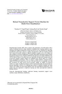
function of the distance, as Fig. 1 illustrates. Note that the distance-based penalty factors plotted in Fig. 1 are scaled to range from 0 to 1 so that they can be superimposed with the Gaussian penalty factors. Fig. 2 displays the surface plots of the Gaussian penalty factor with different Gaussian widths, overlaying on a scatter plot of samples drawn from a two-dimensional Gaussian with zero mean and covariance matrix    1 0.8 . 0.8 5   

i

 d should be related to the spread of the samples in the training set. It is estimated as the average of the square roots of the eigenvalues of the retained PCs, i.e. 1 l (14)  d   i l i 1 3) In the testing process, the test sample is first normalised by the mean and standard deviation of training samples, and then evaluated by the built model to obtain its predicted label.

1 Distance-based Gaussian-based (width = 0.38) Gaussian-based (width = 1)

0.8

0.6

0.4

III. SIMULATION RESULTS In this section, we conduct two groups of experiments to verify the performance of the one-class SVM and the robust one-class SVMs. The Iris’ Fisher dataset and the banana data set are selected to perform the experiments and compare the accuracies of the traditional one-class SVM, the robust one-class SVM proposed by [3] (ROCSVM), and our Gaussian-based robust one-class SVM model.

0.2

0

0

5

10

15

Fig. 1. Distanced-based and Gaussian-based penalty factors as a function of 2-norm distance between the samples and the centre of the data.

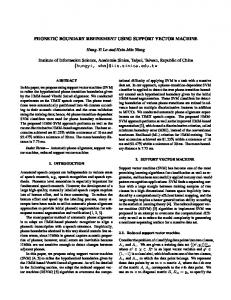
A. Case I: Iris’ Fisher Dataset The data that we used in this experiment are obtained from Iris’ Fisher dataset which contains 50 samples of 3 types of Iris flower. Two species, the Iris versicolor and Iris verginica with petal length and petal width feature, are selected to perform the experiment. Here we select the Iris versicolor as the positive class (normal class), and the verginica species as the negative class. From the scatter plot in Fig. 3, we can clearly see that the two classes are quite poorly-separated. We execute 50 runs of experiments. For each run, thirty samples of positive class are included in the training set and the remaining twenty samples are for testing. To evaluate the robustness of the considered techniques against outliers, 10% (3 samples) and 20% (6 samples) of negative samples are randomly picked and contaminated in the training set.

(a) (b) Fig. 2. Gaussian-based penalty factor surface for normal distributed dataset (a) width = 1 (b) width = 0.38.

It can be seen that the value of Gaussian width has a great influence on the distribution of the penalty factors and, as a result, affects the final outcome of this robust one-class SVM. In this work, we propose to estimate the Gaussian width of penalty factors as a function the eigenvalues of the PCA-projected data. The steps of proposed Gaussian-based robust one-class SVM can be summarised as follows: 1) The original training samples are scaled to zero mean and unitary standard deviation. The scaled data are preprocessed by PCA (principal component analysis) which decomposes the scaled training matrix X  R Nxm as X  t1p1T  t 2pT2  ...  t l pTl  E

(12)

where ti is the scores vector, pi is the loading vector, l is the number of principal components (PCs) retained in PC model, and E is the residual matrix. The loading vector pi can be computed as the ith eigenvector of the covariance matrix cov(X) and i is the eigenvalue corresponding to the eigenvector pi. The scores vector t i  R l represents the

Fig. 3. Scatter plot of the features selected Iris’ Fisher dataset before the PCA preprocessing.

projections of the scaled data sample x along the PCs. The score matrix T corresponding to the projections of the scaled training matrix X can be calculated as: T  X[p1 p 2  p l ], T  R Nxl

Twenty samples of the remaining negative data points are included in the test set. Therefore, in the test set there are 20 samples from the positive class and 20 samples from the negative class. All data are normalised before training and testing as described in the method section. For one-class SVM, the regularisation parameter   0.05 . The constant  of all robust one-class SVM techniques is set

(13)

2) The robust one-class SVM model is developed by 148

International Journal of Materials, Mechanics and Manufacturing, Vol. 5, No. 3, August 2017

to 1 / N to make an equivalent comparison. For each run, the width parameter  for Gaussian kernel is varied from 0.5 to 8.0 with step size of 0.5 and the corresponding classification accuracy when tested on the test set is computed. After 50 executions, we select the optimal kernel parameter for each SVM technique from the one that gives the best performance, i.e. the highest average accuracy. The best average accuracies obtained from all SVM models are listed in Tables I and II, where standard deviations are given in brackets. We also analyse the difference between the proposed method and the others by the Wilcoxon signed-ranks test [8]. The last two rows in the tables list the test results and their p-values, where h = 1 indicates that there is significant difference between the proposed method and the other, while h = 0 indicates when there is not.

To compare the performances of all considered SVM methods when the training data are contaminated by outliers, their decision boundaries for 10% contamination case are shown in Fig. 4. The proposed robust one-class SVM results are in good performances on this dataset. It apparently shows that the outliers fall outside of the decision boundary. In contrary, the decision boundaries of one-class SVM and ROCSVM are loose and shifted towards the outliers. From the results in Tables I and II, it is apparent that the proposed method is superior to the other methods on all cases of Iris’ Fisher dataset. Specifically, among the three methods, the proposed method obtains the highest accuracies. B. Case II: Banana Dataset In this experiment, we perform experiment on the dataset which is distributed in banana shape. The banana-shaped data are selected to investigate the performance of the considered SVM techniques in non-Gaussian distributed data.

TABLE I: PERCENT ACCURACIES FOR IRIS’S FISHER DATASET WITH  = 0.05, OUTLIERS = 10% Dataset Iris’ Fisher p-Value h

OCSVM 79.05(7.16) 1.20  10-7 1

ROCSVM 79.05(7.16) 1.20  10-7 1

Proposed 86.40(5.28) -

TABLE II: PERCENT ACCURACIES FOR IRIS’S FISHER DATASET WITH  = 0.05, OUTLIERS = 20% Dataset Iris’ Fisher p-Value h

OCSVM 73.25(7.46) 1.89  10-9 1

ROCSVM 73.25(7.46) 1.89  10-9 1

Proposed 87.60(6.10) -

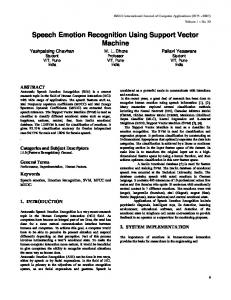
Fig. 5. Scatter plot of the banana dataset and outliers before the PCA preprocessing.

4

decision boundary training data outliers

3 2 1

The banana-shaped dataset contains 150 samples of positive samples and 100 samples of Gaussian-distributed negative class. In Fig. 5, the scatter plot of positive and negative samples for this dataset shows that the two classes are clearly separable. The training data are composed of 100 randomly selected positive samples contaminated with 10% (10 samples) and 20% (20 samples) from the negative class. To construct test data, 50 samples from the banana dataset and 50 samples from the Gaussian ones which are not already included in the training set are randomly selected. For one-class SVM, the regularisation parameter   0.05 and a constant   1/ N is used for the two robust SVM methods. The width parameter for Gaussian kernel is varied from 0.5 to 8.0, with step size of 0.5 and the corresponding classification accuracy for the testing samples is computed. Tables III and IV show the best accuracies averaging from 50 runs with standard deviations and the results of the Wilcoxon signed –ranks test also being displayed.

0

0

0

0

0 0

-1 -2 -3 -4 -5

0

5

(a) OCSVM 79.50% accuracy, width = 1.0 4

decision boundary training data outliers

3 2 1

0

0

0

0

0

0

-1 -2 -3 -4 -5

0

5

(b) ROCSVM 79.50% accuracy, width = 1.0 4

decision boundary training data outliers

3 2

TABLE III: PERCENT ACCURACIES FOR BANANA DATASET WITH  = 0.05, Outliers = 10%

1 0

Dataset Banana p-Value h

0

0

0 -1 -2

OCSVM 62.98(7.80) 7.46  10-10 1

ROCSVM 61.78(6.87) 7.47  10-10 1

Proposed 89.18(3.41) -

-3 -4 -5

0

To illustrate the performance of the three methods on the banana-shaped dataset, we plot their decision boundaries in Fig. 6. The decision boundaries of one-class SVM method and ROCSVM are apparently loose; the decision boundaries

5

(c) Proposed 89.20% accuracy, width = 6.5 Fig. 4. Scatter plots of contaminated training set of the Iris data and the resulting decision boundaries of (a) OCSVM, (b) ROCSVM, and (c) the proposed method using the optimal kernel widths.

149

International Journal of Materials, Mechanics and Manufacturing, Vol. 5, No. 3, August 2017

in Fig. 6(a) and 6(b) are likely to shift towards the outliers. It is clearly shown in Fig. 6(c) that the method we proposed is capable of describing the banana-shaped dataset contaminated with outliers accurately

bearing fault dataset to illustrate its applicability in practice. The comparison with other two methods, i.e. the OCSVM and ROCSVM, is also made A. Experiment Dataset The bearing data were obtained from the Society for Machinery Failure Prevention Technology (MFPT) [9]. The time-domain vibration signals of bearing were collected from the normal case, outer race fault case, and the case of inner race fault with input shaft rate of 25Hz [10]. The vibration signal collected from different fault conditions and different sampling rate were divided into non-overlapping 0.15-second width windows. The details of this dataset are listed in Table V.

TABLE IV: PERCENT ACCURACIES FOR BANANA DATASET WITH  = 0.05, OUTLIERS = 20% Dataset Banana p-Value h

OCSVM 57.28(5.06) 7.36  10-10 1

ROCSVM1 55.80(4.73) 7.36  10-10 1

Proposed 90.80(3.02) -

4

3

2 0

0

TABLE V: DETAILS OF MFPT BEARING FAULT DATASET Sampling Number of Data length Condition class frequency samples (samples) (Hz) Normal condition 120 97.6 14,648 Outer race fault 120 97.6 14,648 Inner race fault 140 48.8 7,324 Other Outer race fault 140 48.8 7,324

1

0

-1 0

decision boundary training data outliers

-2

-3

-4 -4

-3

-2

-1

0

1

2

3

4

(a) OCSVM 58.00% accuracy, width = 1.0

Bearing enveloped analysis which is a well-known signal processing technique for bearing fault detection was applied to extract the fault features. We used the envelope kurtosis with frequency bands 1 kHz to 4.05 kHz and 1 kHz to 9.1 kHz to construct a set of two-dimensional features representing the three fault conditions.

4

3

2 0

1

0

0

-1

0

decision boundary training data outliers

-2

-3

-4 -4

-3

-2

-1

0

1

2

3

4

(b) ROCSVM 58.00% accuracy, width = 1.0 4

3

2

Fig. 7. Scatter plot of features of MFPT dataset before the PCA preprocessing.

1 0 0

0 0

Scatter plot of features in Fig. 7 shows that the normal dataset is clearly separable from the other two faulty datasets, while the outer race and inner race fault data are poorly separated. In this experiment, we consider three cases as follows: Case I: Normal as positive class and inner race faulty as negative class 60 samples of normal condition of bearing are randomly selected in the training dataset which is contaminated with 10% (6 samples) and 20% (12 samples) of inner race fault data. The testing data is constructed by randomly selected 60 data points from normal condition of bearing and 60 data points from inner race fault bearing. Case II: Inner race fault as positive class and outer race fault as negative class 60 samples of inner race fault data are randomly selected in the training dataset which is contaminated with 10% (6 samples) and 20% (12 samples) of outer race fault data. The testing data is constructed by randomly selected 60 data points from inner race fault condition and 60 data points from outer race fault bearing.

-1

decision boundary training data outliers

-2

-3

-4 -4

-3

-2

-1

0

1

2

3

4

(c) Proposed 87.00% accuracy, width = 0.9 Fig. 6. Scatter plots of contaminated training set of the banana data and the resulting decision boundaries of (a) OCSVM, (b) ROCSVM, and (c) the proposed method using the optimal kernel widths.

From the results in Tables III and IV, it is apparent that the proposed method is superior to the other methods for all levels of outliers. Specifically, it can be observed that the Gaussian-based robust one-class SVM performs equally well for 10% and 20% outlier contamination cases with accuracies approximately 90%. On the contrary, the OCSVM and ROCSVM greatly suffer from the increasing level of outlier contamination.

IV. APPLICATION TO MFPT BEARING FAULT DATASET In this section, the proposed technique is tested on the 150

International Journal of Materials, Mechanics and Manufacturing, Vol. 5, No. 3, August 2017

Case III: Outer race fault as positive class and inner race fault as negative class: 60 samples of outer race fault data are randomly selected in the training dataset which is contaminated with 10% (6 samples) and 20% (12 samples) of inner race fault data. The testing data is constructed by randomly selected 60 data points from outer race fault condition and 60 data points from inner race fault bearing. In each case, the regularisation parameter  is set at 0.05 for one-class SVM and   1/ N for all robust one-class SVM. Again, the optimal kernel widths are obtained by performing the grid search over the range of 0.5 – 8.0 and considering the average accuracy over 50 executions as the performance index of the search. Case I represents the case where the contaminated outliers are far away from the positive case.

outliers and the positive samples are close which make it difficult to define an appropriate decision boundary. The results of both cases are shown in Tables VIII – XI with corresponding boundaries plotted in Figs. 9 and 10. It can be clearly observed that even in such difficult cases where the contaminated outliers are poorly-separated from the actual positive samples; the proposed method can still provide satisfying results. 4

decision boundary training data outliers

3 2 1

0

0

0 0

0

-1 0

-2 0

-3

B. Result The results of Case I are listed in Tables VI and VII. Overall, the average accuracy of the proposed method is higher than accuracies of the other two methods for both 10% and 20% contamination levels.

-4 -4

-2

ROCSVM 89.78(4.23) 5.14  10-9 1

2 1

OCSVM 80.50(6.28) 7.49  10-10 1 4

2 1

-4 -4

Dataset Bearing p-Value H

Dataset Bearing p-Value h

0

0

-3

0

2

4

6

8

decision boundary training data outliers

3 2

Dataset Bearing p-Value h

1 0

0

0

4

6

8

OCSVM 70.20(5.10) 7.47  10-10 1

ROCSVM1 70.20(5.10) 7.47  10-10 1

Proposed 86.10(3.41) -

OCSVM 63.95(5.68) 7.98  10-10 1

ROCSVM1 63.95(5.68) 7.98  10-10 1

Proposed 81.57(5.02) -

TABLE X: PERCENT ACCURACIES FOR CASE III WITH  = 0.05, OUTLIERS = 10%

(a) ROCSVM 89.78% accuracy, width = 0.5 4

2

TABLE IX: PERCENT ACCURACIES FOR CASE II WITH  = 0.05, OUTLIERS = 20%

0

-2

0

TABLE VIII: PERCENT ACCURACIES FOR CASE II WITH  = 0.05, OUTLIERS = 10%

Proposed 96.48(2.26) -

-2

-4 -4

-2

(b) Proposed 95.83% accuracy, width = 6.5 Fig. 9. Scatter plots of contaminated training set of Case II bearing dataset and the resulting decision boundaries of (a) ROCSVM, and (b) the proposed method using the optimal kernel widths.

0 -1

0

-3

decision boundary training data outliers

3

8

-2

Proposed 96.32(1.99) -

ROCSVM 80.50(6.28) 7.49  10-10 1

6

0

-1

TABLE VII: PERCENT ACCURACIES FOR CASE I WITH  = 0.05, OUTLIERS = 20% Dataset Bearing p-Value h

4

decision boundary training data outliers

3

TABLE VI: PERCENT ACCURACIES FOR CASE I WITH  = 0.05, OUTLIERS = 10% OCSVM 89.78(4.23) 5.14 10-9 1

2

4

0

Dataset Bearing p-Value h

0

(a) ROCSVM 75.00% accuracy, width = 1.0

OCSVM 69.48(4.74) 7.49  10-10 1

ROCSVM1 69.48(4.74) 7.49  10-10 1

Proposed 83.78(3.47) -

-1 -2

TABLE XI: PERCENT ACCURACIES FOR CASE III WITH  = 0.05, OUTLIERS = 20%

-3 -4 -4

-2

0

2

4

6

Dataset Bearing p-Value h

8

(b) Proposed 96.32% accuracy, width = 1.0 Fig. 8. Scatter plots of contaminated training set of Case I bearing dataset and the resulting decision boundaries of (a) ROCSVM, and (b) the proposed method using the optimal kernel widths.

Fig. 8(a) shows that the decision boundary of ROCSVM is tight and the ROCSVM mistakes the outliers as positive classes. The increased number of falsely identified positive samples deteriorates the overall accuracy as a result. For Cases II and III, we explore the situations where the

OCSVM 63.65(5.81) 1.29  10-9 1

ROCSVM1 63.65(5.81) 1.29  10-9 1

Proposed 77.97(5.17) -

In general, the Gaussian-based penalty factors are more robust to the samples that are far from the centre of the data points and try to force them to be outside the decision boundary. However, it can also misidentify the actual positive samples which happen to be located further from the centre. 151

International Journal of Materials, Mechanics and Manufacturing, Vol. 5, No. 3, August 2017

Having said that, from all of the investigated cases which represent both close and far outliers we may conclude that the proposed penalty function has good potential to be used in practice.

parameter selection for Gaussian kernel when being incorporated with the proposed robust one-class SVM. REFERENCES M. A. F. Pimentel, D. A. Clifton, L. Clifton, and L. Tarassenko, “A review of novelty detection,” Signal Processing, vol. 99, pp. 215-249, June 2014. [2] B. Scholkopf, J. C. Platt, J. Shawe-Taylor, A. J. Smola, and R. C. Williamson, “Estimating the support of a high-dimensional distribution,” Neural Computation, vol. 3, no. 7, pp. 1443-1471, July 2001. [3] S. Yin, X. Zhu, and C. Jing, “Fault detection based on a robust one class support vector machine,” Neurocomputing, vol. 145, pp. 263-268, December 2014. [4] B. Scholkopf, R. C. Williamson, A. J. Smola, J. Shawe-Taylor, and J. C. Platt, “Support vector method for novelty detection,” Advances in Neural Information Processing Systems, vol. 13, pp. 582-588, 2000. [5] S. S. Keerthi and C. J. Lin, “Asymptotic behaviors of support vctor machines with gaussian kernel,” Neural Computation, vol. 15, no. 7, pp. 1667-1689, July 2003. [6] M. Liu, B.C. Vemuri, S.-I. Amari, and F. Nielsen, “Total bregman divergence and its applications to shape retrieval,” in Proc. IEEE Conference on Computer Vision and Pattern Recognition, 2010, pp. 3463-3468. [7] S. Yin and G. Wang, “A modified partial robust M-regression to improve prediction performance for data with outliers,” in Proc. IEEE International Symposium on Industrial Electronics, 2013, pp. 1-6. [8] J. Demsar, “Statistical comparisons of classifiers over multiple data sets,” The Journal of Machine Learning Research, vol. 7, pp. 1-30, 2006. [9] E. Bechhoefer. Condition based maintenance fault database for testing of diagnostic and prognostics algorithms. [Online]. Available: http://www.mfpt.org/FaultData/FaultData.htm [10] E. Bechhoefer, P. Menon, and M. Kingsley, “Bearing envelope analysis window selection using spectral kurtosis techniques,” in Proc. IEEE Conference on Prognostics and Health Management, Montreal, 2011, pp. 1-6. [1]

decision boundary training data outliers

4

0

0

0

3 2 1

0

0

0

0 -1

0

-2 -3 -4 -4

-2

0

2

4

6

8

(a) ROCSVM 69.48% accuracy, width = 0.5 decision boundary training data outliers

4 3 2

0

1 0

0 0

-1 -2 -3 -4 -4

-2

0

2

4

6

8

(b) Proposed 83.78% accuracy, width = 8.0 Fig. 10. Scatter plots of contaminated training set of Case III bearing dataset and the resulting decision boundaries of (a) ROCSVM, and (b) the proposed method using the optimal kernel widths.

V. CONCLUSIONS In this paper, we study the robustness of one-class SVM and its application to fault detection. We propose a novel method of penalisation that can decrease the influences of outliers by using adaptive penalty factor. The robust one-class SVM presented in literature (ROCSVM) solves the problem by adjusting the penalty factor based on the distance between the data point and the centre coordinate of the data set. However, this method is unable to make full use of the data distribution information. Therefore, the Gaussian function which makes use of the distribution of the data is proposed to adjust the penalty factor. Then we test the performances of methods using three groups of experiments: Iris’ Fisher dataset, banana-shaped dataset, and MFPT bearing fault dataset which is a practical industry dataset. Outliers are apparently contaminated in the training data to evaluate the robustness of each method. As shown by the experimental results, the proposed robust one-class SVM can generate the suitable decision boundaries and perform much better than other methods. However, currently the width parameter for Gaussian kernel is exhaustedly searched by using the grid search for the sake of fair comparison which is clearly not possible in practice. Future research will be focused on the study of the

T. Prayoonpitak received the BEng degree in electrical engineering from King Mongkut's Institute of Technology Ladkrabang, Bangkok, Thailand, 2007. He is currently an MS degree student in King Monkut’s University of Technology Thonburi, Bangkok, Thailand. His research interests include fault classification and machine learning.

S. Wongsa received the BEng degree in control systems and instrumentation from King Monkut’s University of Technology Thonburi, Bangkok, Thailand in 1998, and the MSc and PhD degrees in automatic control and systems engineering from Sheffield University, United Kingdom, in 2002 and 2007, respectively. She is currently an assistant professor in the Department of Control Systems and Instrumentation Engineering at King Monkut’s University of Technology Thonburi. Her research interests include intelligent fault detection and diagnosis.

152