1
A Scale-based Connected Coherence Tree Algorithm for Image Segmentation ∗
Jundi Ding1 , Runing Ma2 , Songcan Chen1 ,
Abstract— This paper presents a connected coherence tree algorithm (CCTA) for image segmentation with no prior knowledge. It aims to find regions of semantic coherence based on the proposed ε-neighbor coherence segmentation criterion. More specifically, with an adaptive spatial scale and an appropriate intensity-difference scale, CCTA often achieves several sets of coherent neighboring pixels which maximize the probability of being a single image content (including kinds of complex backgrounds). In practice, each set of coherent neighboring pixels corresponds to a coherence class (CC). The fact that each CC just contains a single equivalence class (EC) ensures the separability of an arbitrary image theoretically. In addition, the resultant CCs are represented by tree-based data structures, named connected coherence tree (CCT)s. In this sense, CCTA is a graph-based image analysis algorithm, which expresses three advantages: (1) its fundamental idea, ε-neighbor coherence segmentation criterion, is easy to interpret and comprehend; (2) it is efficient due to a linear computational complexity in the number of image pixels; (3) both subjective comparisons and objective evaluation have shown that it is effective for the tasks of semantic object segmentation and figure-ground separation in a wide variety of images. Those images either contain tiny, long and thin objects or are severely degraded by noise, uneven lighting, occlusion, poor illumination and shadow. Index Terms— ε-neighbor coherence segmentation criterion, connected coherence tree, semantic segmentation, object segmentation, figure-ground separation.
I. I NTRODUCTION Image segmentation is an extensively studied area with a long history. It is perhaps the most challenging and critical problem in image processing and analysis. The principal difficulty encountered in image processing is the ability of techniques to extract semantic objects correctly from an image with no prior knowledge. Many other video processing applications suffer from the same drawback, such as MPEG-4 [1] and query by image databases [2] of MPEG-7. Therefore, it is significant to propose a semantic segmentation algorithm. Once a number of semantically salient and meaningful regions have been identified, it is possible to quantify their locations and spatial organizations correlatively. That is a crucial factor in the interpretation process, e.g. a blue extended patch at the top of an image probably represents a clear sky (see also [3], [4]). Namely, the segmentation results can be further used for image, video coding and their retrievals, or other intermediatelevel and high-level processings in computer vision, such as ∗ Corresponding
author. Email:
[email protected] of Computer Science & Engineering, Nanjing University of Aeronautics & Astronautics, Nanjing, 210016, P.R. China 2 Department of Mathematics, Nanjing University of Aeronautics & Astronautics, Nanjing, 210016, P.R. China 1 Department
figure-ground separation, blob-detection, and contour completion [5], [6]. Numerous methods have already been proposed for image segmentation, which vary from k-means algorithm to thresholding procedures, to heuristic region growing processes, and to the sophisticated hierarchical methods [7], [8]. K-means algorithm, the best known and most widely used clustering method, is unable to handle unbalanced elongated clusters, where one cluster has much more points than a neighboring cluster. In those cases, the k-means algorithm will erroneously split the larger cluster into artificial sub-clusters. Image thresholding methods are also popular due to their simplicity and efficiency. However, traditional histogram-based thresholding algorithms cannot separate those areas which have the same gray level but do not belong to the same part. In addition, they cannot process images whose histograms are nearly unimodal, especially when the target region is much smaller than the background area. Region growing algorithms deal with spatial repartition of the image feature information. In general, they perform better than the thresholding approaches for several sets of images. But the typical region growing processes are inherently sequential. The regions produced depend both on the order in which pixels are scanned and on the value of pixels which are first scanned and gathered to define each new segment. Hierarchical methods, such as the split-andmerge techniques, often yield strong artifacts in segmentation: the region borders have ragged appearance; long, thin, waving objects are difficult to delineate. These issues pointed out above have reflected that the problem of image segmentation is important and difficult. Furthermore, there is no crisp definition of the concept itself. The only stable definition of segmentation is the statement of the ultimate goal: finding regions of semantic coherence [9]. As pointed out by many researchers in [10]–[23], segmentation procedures based on graph theoretic considerations have a better favoring potential for fulfilling the above requirements than the methods mentioned above. Their hierarchical natures facilitate the subsequent processing and analysis of images. S. Makrogiannis et al. in [24] contend that these diversified graph-based methods coming forth in recent years use the Gestalt principles of perceptual grouping to form the image regions. They commonly represent an image to be segmented as a graph. The nodes correspond to the image pixels, the edges(branches) convey the relations between pixels by a weight which indicates the (dis)-similarity of the two pixels (or regions). The graph-based methods here are roughly divided into two categories: tree-structured segmentation [10]–[16] and spectral
2
clustering [17]–[22]. Both try to divide the initial graph into subgraphs that correspond to image regions. The former is based on agglomeration heuristics to yield the final treestructured subgraphs via merging or splitting operations. The latter is based on the notion of graph cuts to realize the graph partition by finding the eigen-decomposition of an affinity matrix that defines the similarities between pixels. For example, an efficient algorithm proposed by Felzenszwalb et al. in [10], [11] belongs to the former category, which is based on the structure of the Kruskal’s minimum spanning tree (KMST). It uses the local variation of intensities between neighboring pixels to obtain a neither under- nor over-segmentation. Moreover, its running time is nearly linear in the number of image pixels. Another efficient MST-based algorithm is developed by Haxhimusa etc. in [12], [13] which borrows the Boruvka’s MST principle. Compared with the tree-structured methods, spectral clustering approaches are computationally expensive, such as the graph cut [17], [18], the Andrew [19] or the Weiss’s methods [20] and the normalized cut (Ncut) [21]– [23]. They are proven to be NP-hard. So, we can only find their approximate solutions practically. In the paper, we propose a scale-based connected coherence tree algorithm (CCTA) for semantic object segmentation and figure-ground separation. It is obvious that CCTA falls into the category of the tree-structured segmentation. More importantly, it satisfies a so-called 3-E property: effective, efficient and easy. This coincides with the suggestion stated by Haxhimusa in [12], [13]. That is, a segmentation method should be i) effective to capture perceptually important regions into a hierarchical structure, reflecting global aspects of the image; ii) highly efficient, running in time linear in the number of pixels; iii) easy to interpret and implement. Specifically, CCTA is to find all semantic regions which perceptually delineate salient objects in the image. And such regions are formed by connecting all coherent pixels in a treebased data structure. So it is important for us to determine what sort of image pixels are coherent. Intuitively, it is useful to think of the notion coherence in terms of the intensity difference between locally contiguous pixels. This means that the neighboring pixels with slowly varying intensities are coherent, while the neighboring pixels with sharp varying intensities are incoherent. Such a formulation is easy to interpret and implement. For a mathematical description, we hence introduce a ε-neighbor coherence segmentation criterion. Under such a criterion, CCTA finds several sets of coherent neighboring pixels which maximize the probability of being a single physical object. At the same time, it builds each formed set into a connected coherence tree (CCT) structure. Naturally, the pixels which are not in any CCTs have significant discontinuous intensity values. CCTA pools them into a residual or remaining group. In other words, CCTA is effective to realize a unification of both coherence region segmentation and incoherence group detection. Moreover, it has a nearly linear computational complexity in the number of the image pixels. Hence, we can say that CCTA is efficient according to Haxhimusa stated in [12], [13]: “ a graphbased segmentation algorithm is efficient if it has a linear computational complexity in proportion to the number of
image pixels.” Considering the ultimate goal of image segmentation mentioned above, it is reasonable to assess the effectiveness of a graph-based algorithm with respect to its ability of finding the semantic coherence regions. Besides, the computational complexity is another characteristic of an algorithm. Undoubtedly, a high computation cost will severely hamper the generalization of the algorithm to wide real-time applications. Other than being effective and efficient, it is not pivotal that whether an algorithm has an intrinsic idea easy to interpret and implement or not. However, it would be desirable if an algorithm can provide such an intrinsical easiness as well as the effectiveness and efficiency. The remainder of this paper is organized as follows. Section 2 reviews some related work briefly. Section 3 is to present the ε-neighbor coherence segmentation criterion and several useful related concepts in detail. CCTA with its property analysis is described in Section 4. Extensive experimental comparison results on synthetic and real-world gray images are demonstrated in Section 5. They have shown that the performance of CCTA is superior to that of KMST [10], [11] and Ncut [21], [22]. Two ways of quantitative and objective evaluation are available in Section 6, where the effectiveness of CCTA is verified by not only empirical goodness but also empirical discrepancy. Finally, we conclude the whole paper. II. R ELATED W ORK Our ultimate purpose of the study is to find visually semantic coherent segments which have no adequate mathematic description fitting well with human visual system. Hence, many researchers just start from the intuition of their visual perception and decision process to determine the semantic coherence of regions. There is a certain formal resemblance between our region coherence and the two criteria mentioned below. In Refs [5], [6], Gu defined the region coherence in the following: µ ¶ max({I(p)}) − min({I(p)}) ≤ T, p ∈ R (1) p∈R
p∈R
It checks all the neighboring pixels of region R to figure out whether region R is still coherent if a neighborhood pixel q is inserted into it. If Eq.(1) is satisfied, then the region’s coherence is not destroyed and the pixel q is added to the region R. Such a criterion is prone to an over-segmentation for a region with gradually changing gray value when the change exceeds the threshold T . In Refs [4], X. Chen replaced the above coherence criterion with the below one: |I(p) − I(q)| ≤ T,
p ∈ R, q ∈ N (p)
(2)
where p is the pixel being processed in current region R and q is its neighbor to be processed. If the difference between the two pixels is below the threshold T , q is added to the current region R. Then q is processed in the same way as p. The region will sequentially grow until no new pixel can be added. Obviously, such a criterion can tolerate the gradual change of the regions’ gray value. Each pixel shares the equal importance to grow the region, so it often tends to segment
SHELL et al.: BARE DEMO OF IEEETRAN.CLS FOR JOURNALS
(a)
(b)
(c)
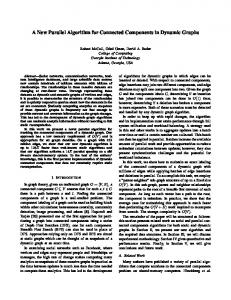
Fig. 1. (a), (b)√and (c) Euclidean neighborhood for ρ =√ 1 (the 4-connected neighborhood), 2 (the 8-connected neighborhood) and 5, respectively. It is obvious that the so-called 8-connected neighborhood is a 3 × 3 square neighborhood.
the regions with low contrast but containing distinct objects into a whole. It thus causes an under-segmentation. Virtually, the algorithmic layout of CCTA has been derived from the modified neighborhood-based clustering (MNBC) algorithm for image segmentation [16] where the generated clusters of grayscales (not the image pixels) are represented by the directed trees (DT)s. The root node of each DT is the seed grayscale whose grayscale neighborhood density factor (GNDF) is not less than 1. The grayscales in k-neighborhood of the root node are its children nodes. Then all the seed grayscales in the children nodes are processed as those in the parent nodes to find their respective children nodes (the grayscales in their respective k-neighborhood). The DT is sequentially growing until no new seed children grayscale can be found. In such a top-down strategy, one DT is constructed beginning with a seed grayscale and terminating at the nonseed children nodes. Dependent on a unique variable k, MNBC can group the grayscales (instead of the image pixels) into one or more DTs. After assigning the corresponding pixels to a constructed DT, one meaningful image region is formed. The pixels with their grayscales not in any DTs are designated as outliers. In this way, MNBC has a linear computational complexity in the number of grayscales in an image. However, it incorporates no spatial information between image pixels. Hence, it cannot tackle the more complex images which are severely degraded by noise, poor illumination and shadow. III. N OTATION AND D EFINITIONS In this section, we would like to introduce several important notations which may be used in the algorithm description in next section. An image I is a pair(I, I) consisting of a finite set I of pixels (points in Z2 ), and a mapping I that assigns to each pixel p = (px , py ) ∈ I a pixel value I(p) in some arbitrary value space. A Square Neighborhood. Experiments have always shown that proximity is an important low-level cue in deciding which image pixels or regions will be grouped. In most imageprocessing applications, it is justified to group the nearby pixels together since they are more likely to belong to the same region. Generally speaking, this cue is characterized by their spatial distance on the image plane. The formal mathematical description is d(p, q) ≤ ρ, ∀p, q ∈ I, where d(p, q) denotes the Euclidean distance and ρ is a specified constant [14]. For a fixed central pixel p, that Np = {q : d(p, q) ≤ ρ, q ∈ I} represents a neighborhood of the pixel p. Figs. 1a, 1b and 1c
3
show the neighboring pixels of a fixed central pixel p in terms of the Euclidean distance between the coordinate values√of pixels, when ρ = 1 (the 4-connected neighborhoods), ρ= 2 √ ( the 8-connected neighborhoods) and ρ = 5, respectively. Note that Fig. 1b is a square neighborhood, which we in this paper focus on. However, it is difficult to use the Euclidean distance to characterize the square neighborhood with a unified expression for the constant ρ. It appears to be able to take √ k 2, k ∈ Z because they are the square neighborhoods when √ k = 1 and √ k = 2. But (k + 1) < k 2 when k ≥ 3, k ∈ Z, i.e. that ρ = k 2 is false. As a result, we have to give a different way to depict the square neighborhood. It is Np = {q ∈ I : |px − qx | ≤ k, |py − qy | ≤ k, k ∈ Z}.
(3)
Obviously, Eq. 3 provides a rigorous mathematical representation for the square neighborhood with the size of (2k + 1) × (2k + 1). The selection of the size for a local square neighborhood determined by k is usually image- and applicationdependent which will be described later. Neighborhood Coherence Factor. Suppose that the square neighborhood of each pixel is given, there are predicatively the pixels in the set Ωp = {q ∈ Np : d(I(p), I(q)) ≤ ε}
(4)
and the pixels in the set Ω0p = {q ∈ Np : d(I(p), I(q)) > ε} (5) S 0 for an arbitrary threshold ε ≥ 0, where Ωp Ωp = Np and d(I(p), I(q)) = |I(p) − I(q)|
(6)
is a pixel-value difference measure. If the intensity difference between a central pixel p and its neighboring pixels is very small (below a threshold), it is conceivable that pixel p will be an interior point of one interested region and could be taken as a seed pixel used to grow the region. In contrast, if the intensity difference between the central pixel p and its neighboring pixels is rather high (above a threshold), the p would be out of one planar surface and lose the growing ability. Intuitively, if the number of neighboring pixels with the intensity values approaching to the central pixel’s exceeds those far away from the central pixel’s, we say that the central pixel could also be taken as a seed because the similar or coherent pixels within its neighborhood are in the ascendant. Motivated by this phenomenological explanation of image formation, we now define one neighborhood coherence factor (NCF) as follows: NCF(p) =
|Ωp | |Ω0p |
(7)
where | · | refers to the cardinality of a set, i.e. the number of elements in a set. It is defined to be the ratio of the number of pixels having the similar intensity with p’s to the number of pixels having the distinct intensity with p’s. Obviously, this value is quite discrepant for different pixels. When |Ωp | ≥ |Ω0p |, NCF(p) ≥ 1. In such a situation, p is similar to most of its neighboring pixels. When |Ωp | < |Ω0p |, NCF(p) < 1. That implies few of its neighboring pixels are similar to p. Therefore, we can say that NCF(p) is actually an
4
(a)
(b)
(c)
(d)
Fig. 2. An illustration of NCF1 : (a) The original image ”Crow” with the size 80 × 120; (b) NCF1 values of image pixels (k = 7, ε = 31); (c) The corresponding NCF1 gray image; (d) Seed pixels in white and no-seed pixels in non-white.
ε-similarity between p and its surrounding pixels with respect to k. Note that |Ω0p | may be 0 and NCF thus becomes infinite. It is necessary for us to give an alternative, NCF1 (p) or NCF2 (p), which are defined in Eq.(8) and Eq.(9) respectively. |Ωp | NCF1 (p) = |Np |
(8)
|Ω0p | |Np |
(9)
NCF2 (p) =
Clearly, when NCF1 (p) ≥ 0.5 the similar pixels will predominate over a handful of discontinuity pixels with sharp varying intensity values. Similarly, when NCF2 (p) ≥ 0.5 the discontinuity pixels with sharp varying intensity values will predominate over the minority similar pixels. Note that NCF1 (p) + NCF2 (p) = 1, hence they complement each other and play an identically important role. Moreover, both NCF1 (p) ≥ 0.5 and NCF2 (p) < 0.5 are equal to NCF(p) ≥ 1. As a result, we can take either of them as a substitute for NCF defined in Eq.(7). In this paper, we use NCF1 (p) to measure the ε-similarity between p and its surrounding pixels. It has the values in the close interval of [0, 1]. In Fig. 2(a-c), we give an example to demonstrate why and how NCF1 can measure the ε-similarity of each pixel to its proximity pixels. From left to right, the three columns respectively show the original natural image named “Crow” with the size 80 × 120, NCF1 values of image pixels (k = 7, ε = 31) and the corresponding NCF1 image in gray. In Fig. 2(a), there are three visible objects: a crow, long and thin branches, and the background. Clearly, the pixels in the background (except for the four angles) have the similar intensities. The pixels around the thin branch or boundary often come from the background and hence have the dissimilar intensities. As we can see in Fig. 2(b), the pixels located in the background have NCF1 values approximating 1 (the maximum in red in the on-line version). It indicates that these pixels are ε-similar to its neighbors. The pixels located on the thin branch and boundary have NCF1 values approximating 0 (the minimum in blue in the on-line version). But note that the
minimum here is 0.0044 = 1/(2 × 7 + 1)2 and Ωp = {p}. It indicates that they are greatly dissimilar with their neighboring pixels. Of course, the pixels lying in the body of the crow have the NCF1 values in the interval (0,1). The corresponding NCF1 gray image is shown in Fig. 2(c). From white to black, the NCF1 values of pixels vary from 1 to 0. Seed pixels. With the analysis detailed above, we can discover that when NCF1 (p) ≥ 0.5, p is ε-similar with its neighbors, i.e., the intensities of majority pixels surrounding p vary slowly; when NCF1 (p) < 0.5, p is distinct from its neighbors, i.e., the intensities of majority pixels surrounding p vary sharply. Further, the pixels with NCF1 (p) ≥ 0.5, together with its nearest neighbors, would delineate all or part of an object with a high probability, as the background pixels in Fig. 2(b-c). Alternatively, the pixels with NCF1 < 0.5 always lie between two different objects which may be the image border or the noise and some shadow boundaries, as the branch pixels in Fig. 2(b-c). Therefore, the pixel p with NCF1 (p) ≥ 0.5 can be taken as a seed pixel to grow the region; whereas the pixel p with NCF1 (p) < 0.5 is called a non-seed pixel. Here, we denote the set of seed pixels as SEED = {p : NCF1 (p) ≥ 0.5, p ∈ I}
(10)
According to this definition, all image pixels are divided into seed pixels and non-seed ones. Fig. 2(d) shows the seed (in white) and non-seed (in black) pixels of “Crow” image (Fig. 2(a)). ε-Neighbor Coherence Segmentation. For any seed pixel p in a region, we say that its ε-neighboring pixels in the set Ωp (see Eq.(4)) are coherent with p which should be in the same region as p. If the pixels within the same region are similar each other, it is likely that the ε-neighbors of any pixel in this region belong to the same part. Let us imagine the opposite case: pick a pixel in a segmented region, whose εneighbors often belong to other regions. Such a segmentation result is useless because it contradicts to the notion of image segmentation, i.e. maximizing the within-region similarities and minimizing the between-region similarities. Hence, we stand out such a sensible observation with the name of “εneighbor coherence segmentation”: For any seed pixel in a current region, its ε-neighboring pixels are coherent and should be segmented into the same region as the seed pixel. More vigorously speaking, the ε-neighbor coherence segmentation defines a “transitive relationship”. Namely, assume p ∈ SEED, q ∈ SEED and t ∈ SEED, if t is one of the εneighbors of q while q is one of the ε-neighbors of p, t together with its all ε-neighbors is grouped into the same region as q and q together with its all ε-neighbors is grouped into the same region as p. In this way, t together with its all ε-neighbors is obviously in the same region as p. In practice, our criterion is motivated by the unsupervised k-nearest neighbor (kNN) consistency in data clustering [25] where the cluster nearest neighbor consistency works as a theoretical foundation. That is, “For any data object in a cluster, its k-nearest neighbors should also be in the same cluster”. Theoretically speaking, our criterion conforms to the cluster kNN consistency. The main task is to identify all points
SHELL et al.: BARE DEMO OF IEEETRAN.CLS FOR JOURNALS
involved in the chain operation and then move them all at once into a cluster or region. The difference is that in kNN consistency, each object is enforced to be a member of a cluster with its kNNs, no matter whether it is an outlier or not; while in our case, only the seed pixels have the ability to grow a region. Hence, our ε-neighbor coherence criterion could reduce the effect or compact of outlier or noise pixels for segmentation and even detect the outlier or noise successfully. Moreover, our criterion could virtually specify an equivalence relation on the set of seed pixels and thereby ensure the separability of an arbitrary image with respect to k and ε. Equivalence Relation. For seed pixels p, q ∈ SEED, we define p ∼ q if p, q satisfy either of the following conditions: (1) p is one of the ε-neighbors of q, i. e. p ∈ Ωq ; (2) There exists a finite number of pixels p1 , · · · , pn such that p ∈ Ωp1 , pk ∈ Ωpk+1 , k = 1, · · · , n − 1, pn ∈ Ωq . It is easy to prove that such a definition satisfies three properties: reflexive, symmetric and transitive. (`ı) reflexive: ∀p ∈ SEED, p is coherent with itself, i.e., p ∈ Ωp , then p ∼ p ; (`ı`ı) symmetric: ∀p, q ∈ SEED, if the pixel-value difference between p and q is under the threshold ε, then q ∈ Ωp and p ∈ Ωq , that is, they are coherent with each other, i.e., q ∼ p implies p ∼ q; (`ı`ı`ı) transitive: ∀p, q, t ∈ SEED, t ∼ q, q ∼ p, then t ∼ p (see the detailed explanation above). It is to say that on the non-empty set of the seed pixels, our segmentation criterion is an equivalence relation ∼. In set theory, equivalence relation is one of the most commonly used and pervasive tools because of its power to partition a given set into the disjoint union of subsets, i.e., Partition Theorem [26]: Let X be a non-empty set and ∼ an equivalence relation on X. The equivalence classes of ∼ form a partition, a disjoint collection of non-empty subsets whose union is the whole set of X. Furthermore, if two seed pixels r, s belong to the same segmented region R (which implies r ∼ s), we can arbitrarily pick one of them as the initial pixel to generate the same region R. That is, our criterion is insensitive to the order of the initial seed pixel selection. Equivalence Class and Coherence Class. As discussed above, the ε-neighbor coherence segmentation shows an equivalence relation among the seed pixels in SEED. Consequently, such an equivalence relation ∼ can partition SEED (the seed pixels) into several equivalence classes (EC). By Partition Theorem, every collection of ECs induced by this equivalence relation ∼ is a partition of the set of seed pixels and thereby a partition of a given image. The number of the equivalence classes determines the number of the expected regions. Moreover, we could pick an arbitrary pixel within the same equivalence class to yield the same region. The analysis and the related concepts above have indicated that our ε-neighbor coherence segmentation criterion guarantees the separability of an arbitrary image. This also suggests that the criterion is reasonable and feasible for the task of image segmentation. Note that the expected final regions are coherence classes, rather than equivalence classes. Because the proposed mean-
5
TABLE I S EGMENTATION ALGORITHM Input: I= (I, I), k Output: all CCTp s and Gr 1. Calculate ε = Ave(k) in Eq. (11), Ωp and NCF1 (p) to obtain SEED; 2. While SEED 6= ∅, ∀p ∈ SEED is a root node to construct CCTp : 2.1 CCTp = Ωp ; 2.2 Q = SEED ∩ (Ωp \ {p}); 2.3 While Q 6= ∅, CCTp = CCTp ∪ (∪q∈Q Ωq ); 2.3.1 Q = SEED ∩ (∪q∈Q Ωq ) \ Q; 2.3.2 End 2.4 Output CCTp ; 2.5 SEED = SEED \ (SEED ∩ CCTp ); 2.6 End 3. Gr = I \ (∪CCTp ); 4. Output Gr .
ingful ε-neighbor coherence segmentation criterion is to group the all ε-neighbors of each seed pixel in the current region into the same region, including the non-seed ε-neighbors of each seed pixel. While these non-seed ε-neighbors without the capability of growth just provide the termination condition of the region growing process. Without loss of generality, we take p as the initial seed pixel to grow one region. Then the set of pixels in I that are grouped into the same expected region as p based on ε-neighbor coherence segmentation criterion is called the coherence class (CC) of p (p’s CC), containing the p’s EC. IV. C ONNECTED C OHERENCE T REE A LGORITHM (CCTA) Remarkably, those foregoing notations and definitions are significant which ensure the separability of an image. That is, the task of dividing an image is equivalent to a job of finding these coherence classes (CCs) according to the εneighbor coherence criterion. Each CC can be represented by a tree-based structure (N,B) with our segmentation algorithm, where N is the set of nodes corresponding to the image pixels in one CC and B is the set of the tree branches connecting all the pixels in one CC. Hence, this tree is called connected coherence tree (CCT). Particularly, the oriented branches describe the ε-coherence relationship between nodes (parent and child): given p1 , p2 ∈ I, (p1 , p2 ) ∈ B means that (1) p1 is a seed node as parent; (2) p2 is a child of p1 and coherent with p1 , i.e., p2 ∈ Ωp1 . Note that, p2 could be one seed or non-seed pixel. If p2 is a non-seed pixel, it would be a leaf node of one CCT; otherwise an interior node which can be used to continue spanning the CCT. Therefore, the nodes of one CCT are the pixels in one CC, where the pixels in the corresponding EC are interior nodes except that the initial seed pixel is the root one and the pixels in CC \ EC are leaf ones. The pixels not in any CCTs will be grouped together as a residual group, denoted as Gr . Table I gives our algorithm. Concretely, all CCTs would be formed in step 2 via the procedure of two closed “while” loops. In the outer “while” loop, Step 2.1 generates the elementary CCTp where the root node is the seed pixel p and its children nodes are the pixels in Ωp \ {p}; Step 2.2 searches for the seed pixels within the children nodes to continue spanning the current CCTp ; Step 2.3 is the inner “while” loop which is to discover all pixels that are reachable from the found
6
TABLE II
A NUMERICAL EXAMPLE FOR CCTA’ S GROWING PROCESS 98 92 96 94 93 95 94
100 97 99 99 98 99 98
102 102 102 103 100 103 100
104 106 105 104 103 102 104
108 107 107 108 109 109 106
90 90 90 88 91 88 88
90 90 89 91 88 91 89
88 88 65 60 63 90 91
89 88 67 65 61 91 89
2 2 3 3 3 2 2
2 2 2 2 2 2 2
90 90 90 88 88 89 88
91 91 91 90 91 90 89
(a) k = 6, ε = Ave(6)
(b) k = 7, ε = Ave(7)
(c) k = 7, ε = 10
(d) k = 12, ε = Ave(12) (e) k = 18, ε = Ave(18) (f) k = 7, ε = 55
⇓ 1 1 1 1 1 1 1
1 1 1 1 1 1 1
1 1 1 1 1 1 1
1 1 1 1 1 1 1
1 1 1 1 1 1 1
2 2 2 2 2 2 2
2 2 2 2 2 2 2
2 2 3 3 3 2 2
2 2 2 2 2 2 2
Fig. 3. The original image is in the left, and the corresponding segmented image is in the right when k = 1, ε = 5 ≈ Ave(1) = 4.5630 in Eq. (11).
children seed nodes in a top-down breadth-first local search. When there is no presence of seed pixels in the children nodes, the inner “while” loop breaks and one final CCT with root p is put out in step 2.4. Step 2.5 pools the remaining seed pixels into the set SEED and the new outer “while” loop restarts to yield another CCT. The algorithm terminates if all seed pixels are settled (i.e. SEED = ∅). Outside the two closed “while” loop, Step 3 groups the residual pixels into the set Gr while Step 4 outputs the formed CCTs. To understand CCTA more clearly, we demonstrate its growing and labeling process in Table II with a numerical example, where the pixels with the bold intensity are the seeds. The corresponding original and segmented images (k = 1, ε = 5) are shown in Fig.3. A. Parameter Sensitivity to Segmentation Quality Obviously, the ε-neighbor coherence segmentation criterion is fundamental to CCTA. When the criterion is applied properly, the derived segmentation should be a good approximation of the image which can thus capture a comprehensive description for higher level processes. As the criterion is handled impertinently, some salient information may still be extracted, but certain classes of objects may be isolated into very small regions which become invalid for higher level processes. A few questions naturally arise: how sensitive is the criterion to the segmentation quality? Can the best segmentation be found automatically? In answer to the first question, we must observe that our criterion in nature involves two parameters, the spatial scale k and the intensity difference scale ε. Within the same image, different region segmentations could be obtained by using different values for them. To elaborate this problem, we would come back to the image “Crow” shown in Fig. 2(a). Ideally, we wish to form three groups of pixels that belong to visually distinct regions such as the branches, the background
(g) k = 4, ε = Ave(4);
(h)k = 20, ε = Ave(20)
Fig. 4. How does the segmentation result vary with k and ε, where according to Eq. (11), Ave(6) = 29.022, Ave(7) = 31.65, Ave(12) = 41.51, Ave(18) = 50.343, Ave(4) = 23.128 and Ave(20) = 52.313.
and the crow. Figure 4 shows how the segmentation result varies with k and ε. The parameter ε used in Eq.(4) associates with the intensity contrast in the given neighborhood of each pixel. At a low value, only these flat regions with the almost constant intensity may be found. At a high value, these regions with the similar intensities but corresponding to different objects may be segmented into one large region. For example (k = 7), ε = 10 is too low in Fig. 4(c), only the smooth background region (except for the four angles) is found and other pixels remain in the residual group. In contrast, ε = 55 is too high to separate the crow and branches from the background in Fig. 4(f). Therefore, the selection of ε directly affects the segmentation result. One could manually choose a fixed ε for all images or adjust ε for each given image based on the image content. The former has proven to be problematic in our tests because the intensity contrast of objects in different images is often not on the same level. The latter is impractical due to the burden of a large tuning computation. Moreover, the image content were implicitly used as a priori information which would make CCTA be a supervised method. In contrast, we try to find a way to automatically calculate ε without increasing the computation complexity of CCTA. As discussed above, NCF1 (p) defined in Eq.(8) virtually acts as an ε-similarity of each pixel p with its neighboring pixels. That is, ε measures the degree of the similarity between p and one of its neighbor in a relative sense. Of course, the degree of the similarity is related to the absolute intensity difference between p and one of its neighbors. If ε is larger than the mean intensity difference in p’s neighborhood, denoted by Mean(k)p in Eq.(11), p is ε-similar with most of its neighboring pixels. However, the values of Mean(k)p of different pixels are different. It is thus difficult to select a proper ε between two extreme cases, i.e. min(Mean(k)p ) and p∈I
max(Mean(k)p ). Notice that once the neighborhood size k p∈I
is determined, the average value of all Mean(k)p , denoted by Ave(k) in Eq.(11), is a constant which describes a global tendency of the intensity variation.
SHELL et al.: BARE DEMO OF IEEETRAN.CLS FOR JOURNALS
P Mean(k)p =
q∈Np
|I(p) − I(q)| |Np |
7
P ; Ave(k) =
p∈I (Mean(k)p )
|I|
(11)
Intuitively, it should be a good candidate for ε. So we conduct extensive tests with different k with purpose to see whether it is feasible to determine ε by this strategy. For this image, when ε is automatically set to be the Ave(k) with different k varying from 6 to 18, the three objects are accurately distinguished into three semantic regions. Figure 4(a-b, d-e) show four cases, k = 6, 7, 12, 18, respectively. Of course, Ave(k) for ε is not always optimal for each image to be segmented. In practice, the values near Ave(k) for ε sometimes produce the better results. Hence, we determine ε near the Ave(k) in our experiments. In this paper, we can always obtain a satisfactory segmentation by selecting ε in the range [Ave(k) − 8, Ave(k) + 8]. In consequence, k is crucial for a successful segmentation. It determines the size of the square neighborhood defined in Eq.(3). Usually k is related to the size of the objects of interest in the image. For most applications, if too small a neighborhood is chosen, CCTA will be sensitive to noise and produce an over-segmentation. For example, the background in Fig. 4(g) (k = 4) is divided into three small regions. On the contrary, if the neighborhood size is too large, CCTA will have the increasing computational complexity and yield an under-segmentation like Fig. 4(h) (k = 20), where the crow is merged with the branches. Since the size information of objects is often not a known priori, it is difficult to choose an optimal k with respect to object dimensions. Similar to the normalized cuts [21] [22], we also experimentally choose an optimal k in a wide range 1-15 for each image through trial and error. In this paper, an adaptive k in the range of 3-10 has been observed in our experiments. B. Computational Complexity of CCTA For a clear qualitative analysis of the proposed algorithm, we will discuss its computational complexity. The most timeconsuming work is the calculation of Ωp for each pixel in Step 1. Practically, it is not necessary to compute Np and Ωp of the pixels which are in the first and last k rows, columns of the image I(w, h), where w and h are the width and height of the image respectively. Because those pixels would be partitioned into several equivalence classes or the residual group. Let N = (w − 2k) ∗ (h − 2k), M = (2k + 1)2 − 1, k ∈ Z, the running time of calculating all Ωp is O(M N ). In our implementation, k ≤ 12. So it takes nearly O(N ) in proportion to the number of pixels because M ¿ N . In addition, the recursive procedure for constructing all CCTs in Step 2 takes about O(N) since each pixel is scanned once, where N is the total number of pixels in the image I. Besides, the automatical selection for ε requires computing Mean(k)p and Ave(k) which takes O(M N ) like the calculation of Ωp . Therefore, the total computational complexity of CCTA is O(M N ), nearly linear in the number of pixels. According to Y. Haxhimusa [12], [13], we can say that CCTA is an efficient graph-based segmentation approach.
(a)
(b)
(c)
(d)
(e)
(f)
(g)
(h)
(i)
Fig. 5. Segmented results for a noisy 6-rectangle gray image 200 × 299: (a) original image; (b) Gaussian noisy image (mean 0 and standard deviation 25.5) ; (c) Gr ; (d)-(i) 6-CCTs corresponding to the five squares. Parameter settings: k = 6, ε = Ave(6) = 37.7476.
V. E XPERIMENTAL R ESULTS
It is obvious that NCF1 describes a kind of local information and the ε-neighbor coherence segmentation criterion captures a global image representation. That is, like Ncut [21] [22] and KMST [10] [11], CCTA is to reach a global and optimal segmentation going from local image cues. As a consequence, they belong to the same segmentation framework. Ncut, based on spectral graph theory, provides a mechanism for going from pairwise pixel affinities to partitions that maximize the ratio of affinities within a group to that across groups, i.e., the normalized cut criterion. By embedding the normalized cut problem in the real value domain, this criterion is formulated as a generalized eigenvalue problem. Then the eigenvectors are used to construct good partitions of the image. KMST, using the Kruskal’s MST principle, is a greedy region merging algorithm based on intensity (or color) differences between neighboring pixels. It could produce neither under- nor over-segmentations which capture non-local image properties. Moreover, KMST runs in time nearly in the number of image pixels. They are two recently developed graph-based segmentation methods which have already delivered impressive results in a number of challenging images. To evaluate our proposed method, in this section, we thus experimentally carry out extensive comparisons with Ncut and KMST on two types of data. One is the synthetic images, including two synthetic noisy images and three synthetic uneven lighting images; The other is a collection of natural images coming from the Berkeley Segmentation Dataset and some empirically usual tested image database. Both contain a variety of images covering a wide range of viewpoints and illumination angles. In both experiments, only grayscale information between 0 and 255 is used. In addition,the codes of Ncut and KMST are available respectively from the authors. Besides some specific default parameters, both of the two methods depend critically upon several other parameters intrinsic to them. For Ncut, there are two parameters, the number of regions c and the radius of neighborhood r. For KMST, there are also two parameters, a constant t controlling the minimum size component, and the number of pixels s within the minimal region. Appropriate setting of these parameters is a pre-requisite for successful segmentation. To make a fair comparison, we tune them over a wide range of values and carefully select ”optimum” so that each method presents the perspectively best results among the numerous different partitions for each image.
8
(a)
(b)
(c)
(d)
(e)
(f)
(g)
Fig. 6. Segmented results for a noisy 24-small-rectangle gray image 95 × 145: (a) original image; (b) Gaussian noisy image (mean 0 and standard deviation 25.5) (c) Gr ; (d) 24 small rectangle regions segmented one by one; (e) the narrow fence region; (f-g) 25 regions segmented by Ncut and KMST respectively. Parameter settings of (c)-(e): k = 2, ε = Ave(2) = 42.2277 for CCTA; (f): c = 25, r = 13 for Ncut; (g): t = 500, s = 500 for KMST.
A. Experiments on Synthetic Images In this subsection, to assess the effectiveness of our algorithm for segmentation tasks, we first perform some experiments on synthetic data: synthetic noisy images and synthetic uneven lighting images. In the interest of ensuring that these synthetic images are biased as little as possible by our immediate research purpose, we intend to collect the complex synthetic images from literatures which contain long, thin and small objects. Besides, they are known to be more challenging and difficult due to the background degraded by noise, uneven lighting, poor illumination and shadow. 1) Results for synthetic noisy images: In [27], Huber pointed out that small deviations from the model assumptions should impair the performance of the algorithm only by a small amount. Here, we employ two synthetic noisy images to illustrate that CCTA, as an image analysis algorithm has an important quality, i.e. resistant to noise. The first noisy image in Fig. 5(b) is with the independent gaussian noise (mean 0 and standard deviation 25.5). Its clean image in Figure 5(a) comprises six equal rectangular-shaped regions whose intensity values vary slowly from dark to white, i.e. the contrast of each region decreasing gradually from left to right. As expected, CCTA successfully yields six CCTs which correspond to the six semantic rectangular-shaped regions when k = 6, ε = Ave(6), as shown in Fig. 5(d)-(i). Little residual noise in Gr is shown in Fig. 5(c). However, many existing methods could find nearly constant intensity regions and thus they are sensitive to artificially added noise. For more evidence, we test on another synthetic noisy image in Fig. 6(b). It is a more complex image than that in Fig. 5(b). Because the contrast in its clean image (Fig. 6(a)) decreases both from left to right and from top to bottom. So it appears to be an uneven lighting image which presents some challenges in segmentation. The same gaussian noise added in 5(b) provides a higher degree of segmentation difficulty. It is made up of 24 disconnected square regions and a white connected fence region. From Fig. 6, we can see that all the three methods, CCTA, Ncut and KMST, can segment this image into 25 regions correctly. But the results by CCTA are visually the smoothest, while those of Ncut are the coarsest. B. Experiments on Synthetic Uneven Lighting Images As illustrated above, CCTA seems to be able to handle the images with the disturbance of uneven lighting. To further exhibit this effectiveness of CCTA, more concrete experiments are conducted on three uneven lighting images which are
(a)
(b)
(c)
(d)
Fig. 7. Results for three images with the uneven lighting background: (a) input images; (b) segmented images by CCTA (1st row 146 × 145: k = 8, ε = 20, Ave(8) = 25.5491; 2nd row 188×251: k = 9, ε = 18, Ave(9) = 21.8871; 3rd row 241×244: k = 9, ε = 7, Ave(9) = 9.9211); (c) segmented images by Ncut (1st row: c = 2, r = 20; 2nd row: c = 2, r = 11; 3rd row: c = 2, r = 15); (d) segmented images by KMST (1st row: t = 100, s = 100; 2nd row: s = 500, t = 100; 3rd row: t = 200, s = 500.
presented in the first column of Fig.7. The reason for selecting a contour map and a document is that the objects in these images include long, thin lines and the background has large homogenous areas. Moreover, under uneven lighting conditions, many methods may easily result in broken lines due to the thinness of contours or strokes, and large black areas called ghost objects because of homogenous areas. Therefore, there is a need to develop a new technique able to effectively deal with this type of images. In fact, the uneven lighting often exists in the capturing of an image. The authors in [28] analyzed that the main causes for uneven lighting are: (1) the light may not be always stable; (2) the object is so large that it creates an uneven distribution of the light; and (3) the scene is unable to be optically isolated from the shadows of other objects. In general, our target for this type of images is to correctly extract the contour map and document from the complex uneven lighting backgrounds or equivalently separate the backgrounds from the contour map and document. That is to say there should be two expected semantic regions ideally. This implies that the segmented background regions should embrace few or no lines of contour map and words of document, which is a hard job. Figure 7 shows the segmentation results for these three images. From left to right, the four columns show the input images (Fig. 7(a)), segmented results by CCTA, Ncut and KMST, respectively. It can be seen that CCTA separates the complex background (the white area of Fig. 7(b)) well from the objects (the black areas of Fig. 7(b)) when the required number of regions is two. The pixels with large intensity variance belonging to the background are organized in one CCT while the pixels with little intensity variance belonging to the contour map and document objects are pooled in a residual group. In contrast, Ncut and KMST are disabled by such an uneven lighting disturbance. They partition these images into two regions which are difficult to decipher, rather than the two reasonable regions, i.e. one background region and one object region. Hence, we have to increase the number of expected regions for Ncut and KMST so that they could achieve a relative comprehensible grouping of pixels. The resultant segmentations are listed in Fig. 7(c) and Fig. 7(d) which still appear very poor, especially for the contour map
SHELL et al.: BARE DEMO OF IEEETRAN.CLS FOR JOURNALS
(a)
(b)
(c)
(d)
9
(e)
Fig. 8. Results for images with many small objects spreading over a relatively simple background. From left to right, they are input images (a), segmented images by CCTA (b)-(c), Ncut (d) and KMST (e), respectively. Parameter settings: ”Rice”: k = 3, ε = Ave(3) for CCTA; c = 78, r = 12 for Ncut; t = 500, s = 30 for KMST; ”Bacteria”: k = 3, ε = 19, Ave(3) = 11.2960 for CCTA; c = 21, r = 12 for Ncut; t = 400, s = 430 for KMST; ”Coins”: k = 5, ε = Ave(5) for CCTA; c = 11, r = 18 for Ncut; t = 300, s = 1000 for KMST.
images. This sufficiently indicates that CCTA is promising for dealing with these challenging images under the condition of uneven lighting. C. Experiments on Natural Images The natural images are more challenging in that they contain significant variations in scale, illumination conditions (sunny versus overcast), material appearance, and sensor noise. The difficult phenomena of shadows, multiple scales, and translucent vegetation are ubiquitous. We wish to segment the natural images into several spatially coherent groups of pixels corresponding to physically objects in the natural world. With no priori information about the image, it is practically difficult to obtain the good semantic segmentation for an unsupervised approach. However, we empirically show that CCTA has succeeded in doing this task using the proposed criterion. Here, the representative sample images are divided into two types. One type contains the images composed of many grains of target objects, which are much smaller than the background such as the rice, bacteria and coins. The other type comes from the Berkeley Segmentation Dataset [9] which contains a wide range of subject matter, such as the translucent water with surface ripples, the clouded sky, the animals partially occluded by sparse vegetation. 1) Results for natural images with grains of objects: Despite much effort done for natural image segmentation, there are still questions which have not been provided the exciting solutions. For example, in the natural world, we often perceived the scenes where many small objects clutter up a large area and the luminance contrast between them is low. Figure 8 shows three images of such kind. Tiny objects, such as grains of rice, granules of bacteria and pieces of coins, spread over the large background in a random order. In [29] Braga-Neto et al. developed an object-based image analysis technology based on the notion of multiscale connectivity, which can be specially exploited for extracting these tiny objects hierarchically from the complicated background. Although the method has produced impressive results for these complicated images, the inherent systematical theory is too
complicated to understand for non-experts. It would hamper its wide application to other kinds of images. Our algorithm, however, possesses an ε-neighbor coherence criterion which is easy to interpret and comprehend and thus our algorithm could flexibly deal with this type of images. From the top to the bottom, we name the three images in Fig. 8 “Rice”, “Bacteria” and “Coins” respectively. Their segmentation results by CCTA, Ncut and KMST are arranged in the corresponding rows. We formulate the problem in an object segmentation paradigm where the task is to distinguish each visual object from the background in a hierarchical order. Hence, beyond a background region, we wish to partition the three images into 81, 21 and 10 regions corresponding to 81 grains of rice, 21 granules of bacteria and 10 pieces of coins, respectively. As shown in Fig. 8(b), CCTA successfully discovers the twenty-one granules of bacteria and the ten pieces of coins. For “Rice”, our method does not find the total eighty-one grains of rice. For k = 3 and ε = Ave(3), CCTA has found 77 salient grains of rice. Four smallest grains of rice located at the image boundary vanish in the visual perspective. Note that each small piece of coin, granule of bacteria or grain of rice is detected in a single region which is represented by one CCT and presented in Fig. 8(b) one by one. Without stating the desired granularity of control over the number of regions, image segmentation is an ill-posed problem. Since the segmentation of the three images produced by CCTA contains 78, 22 and 11 regions (including one background region) respectively, it is reasonable to enforce Ncut and KMST to also produce results with 78, 22 and 11 regions. Then we compare their segmentation results in a fair manner. Perceptibly, CCTA performs consistently the best. From Fig. 8(b), we can see that each visually desired and small objects are effectively distinguished from the background by CCTA. In addition, Fig. 8(c) has shown that CCTA represents the complex background as a whole by one CCT. That meets our goal of the semantic segmentation, namely, all the objects including the background should be of “approximately equal importance”. KMST also attends to the segmentation of the background areas as seen in Fig. 8(e). However, KMST falsely merges many visually salient small objects into the background regions. Those unfavorable issues also arise in the results segmented by Ncut in Fig. 8(d). Moreover, Ncut often fragments the backgrounds into many meaningless pieces, especially for “Bacteria” which has the white background areas around each granule of bacteria. 2) Results on Berkeley Segmentation Dataset: Distinguishing rice, bacteria and coins from the background is a form of the figure-ground discrimination problem. In this subsection, we apply our algorithm to this problem more directly on seven representative natural images which come from the Berkeley Segmentation Dataset. The most of Berkeley Benchmark images are of animals in natural scenes, but there are also many images of people, man-made structures, and urban scenes. It is known to us that the figure-ground separation problem is hard to solve. The objective is to isolate objects of interest from the background in arbitrary scenes. On one hand, CCTA intends to partition an image into a set of disjointed regions R such that each object Oi is projected
10
Fig. 10. The residual groups of all images. Top row: Gr represents noise (1st column) the semantic object; Lower row: Gr represents the contour or boundaries of object.
(a)
(b)
(c)
(d)
Fig. 9. Results for seven natural images coming from Berkeley database. From left to right, they respectively are input images (a), segmented images by CCTA (b), Ncut (c) and KMST (d). The corresponding parameter settings are ”Crow”: k = 5, ε = 20, Ave(5) = 16, c = 2, r = 13 and t = 500, s = 600; ”Tiny animal”: k = 4, ε = Ave(4), c = 3, r = 13 and t = 100, s = 150; ”Pie”: k = 7, ε = Ave(7), c = 3, r = 20 and t = 800, s = 900; ”Boat”: k = 5, ε = Ave(5), c = 2, r = 11 and t = 300, s = 500; ”Bear”: k = 7, ε = 29, Ave(7) = 35, c = 3, r = 10 and t = 300, s = 300; ”Glede”: k = 10, ε = Ave(10), c = 3, r = 12 and t = 300, s = 200; ”Plane”: k = 8, ε = Ave(8), c = 2, r = 10 and t = 500, s = 500.
into a subset R ⊆ R of these regions. According to the previous descriptive concepts for CCTA, the set of disjointed regions R is certainly composed of several coherence classes (CCs) and a residual group Gr (it is possible that Gr = ∅). The mathematic depiction is that R = CCs ∪ Gr . The notions of EC and CC in the above sections imply that CCTA could be powerful to find each R exactly, which is just coincident with the goal of figure-ground separation. On the other hand, CCTA utilizes a bounded breadth-first search for a set of connected pixels that maximize the probability of being an object. This local search is efficient because of its linear computational complexity, in contrast to Ncut and other graph-based topdown methods [14], [15], [17]–[23]. For convenience, we consider a restricted form of the figure-ground problem, i.e. only one or two classes of objects appears in the scene, like the seven chosen Berkeley Benchmark images-“Crow”, “Tiny Animal”, “Pie”, “Boat”, “Bear”, “Glede” and “Plane”. The background consisting of an arbitrarily large number of real objects from the world is out of our focus. However, the backgrounds of clouded sky, rippled water, poor illumination and shadow in the natural world still present many challenges and difficulties. Comparison results for the seven tested images are shown in Fig.9. From left to right, these columns are the input images, segmentation of CCTA, Ncut (the 2nd column counted from right) and KMST (the rightmost column), respectively. The results are qualitatively different, although the number of regions is identical or similar. While CCTA does not guarantee to find the best solution, it practically performs quite well. It appears that CCTA outperforms Ncut and KMST
consistently. For example, “Tiny Animal” is an image of a tiny animal walking in the snowbank at night. Some disturbing sensor and reflex noise exist in this image. Ncut separates the black noisy sky into two regions and misses the tiny animal. KMST discovers the strip of noise pixels and merges the tiny animal into the sky region and snowbank region in a wrong way. CCTA correctly finds the tiny animal and achieves two apart sky and snowband regions exempted from the annoying disturbance. This example illustrates one of the advantages of CCTA, which is also distinctly exemplified in “Plane”. The complicated clouded sky with sharp intensity variance disables Ncut from finding the flying plane accurately. In contrast, KMST seems to extract a roughened plane which is a distortion of the desired flying plane. Note that large regions with coherent intensity generally do not correspond to the projected surfaces of an object in our experiments. “Crow” is such an image. A crow rests on the long and thin branches and the intensity contrast between them is very low. Simultaneously, the branches divide the background with shadow into several occlusions. For this image, CCTA excellently discriminates the three objects, branches, a crow and the complex background as a whole. While Ncut fails to isolate the crow from the branches and manifests the complex background with two or three different intensity regions. The same issue happens to KMST. The results for other images segmented by Ncut and KMST are much coarser than those by CCTA, especially for “Bear”, an image of a black bear playing in a pond overgrown with float grass. Ncut cannot separate the black bear from the pond, while KMST has the bear and its inverted reflection in water merged together. D. Interpretation of The Residual Group Gr in CCTA In our experiments, CCTA achieves one residual group Gr for each image. Figure 10 depicts the segmented residual groups of all images. Apparently, they represent the rejected noise, contours or boundaries and the undersized objects. As stated in the previous sections, CCTA is to seek for a semantic segmentation based on the proposed ε-neighbor coherence criterion. The coherent neighboring pixels would belong to the same object region with a high probability. The intensity differences between them are below the threshold ε which are thereby connected by branches of one CCT. Meanwhile, the pixels with the highly discontinuous intensity are excluded from being the nodes of any CCTs which are pooled into a residual group. Notably, it often holds true that intensity discontinuities are generally caused by noise, occlusions, object contours, region boundaries and shadow.
SHELL et al.: BARE DEMO OF IEEETRAN.CLS FOR JOURNALS
Hence, we can see that Gr s in Fig.10 delineate noise, object contours or some combination of types of intensity discontinuity. In practice, the tested images in our experiments have the complex backgrounds, such as the clouded sky, scenes fragmented by long and thin branches, or degraded by shadow, uneven lighting, sensor and reflex disturbance. And that, the sizes of objects of the interest and the complex backgrounds are in discrepancy. Those factors lead an impossibility for CCTA to find a suitable spatial neighborhood scale k which would make a tradeoff between the large backgrounds and the small target objects. Rather than to extract objects from backgrounds, CCTA indeed prefers to isolate the perplexing backgrounds from objects of the interest. As we can see, k is often larger relative to the size of objects. Accordingly, the small or tiny animal, long and thin contour map, document words, branches are excluded from the background regions, which are kept in the residual groups. VI. E VALUATION OF E XPERIMENTAL C OMPARISONS Up to now, the effectiveness of CCTA is evaluated visually. In other words, the results of the three methods are only measured qualitatively and indirectly on the extensive difficult images. That is a rather subjective comparison. It is so necessary to provide a reliable objective judgement with a quantitative evaluation method. In [30], Y. J. Zhang divided a variety of segmentation evaluation methods into two categories: analytical methods and empirical methods. “The analytical methods directly examine and assess the segmentation algorithms themselves by analyzing their principles and properties. The empirical methods indirectly judge the segmentation algorithm by applying them to test images and measuring the quality of segmentation results.” Recently, Cardoso etc. in [31] further classified the empirical methods into empirical with implicit reference (so-called empirical goodness) and empirical with explicit reference (so-called empirical discrepancy). The entropy-based quantitative evaluation function E proposed by H. Zhang in [32] falls into the class of empirical with implicit reference. The global consistency measure (GCE) and local consistency measure (LCE) are introduced by Martin in [9], more thoroughly in [33]. They belong to the class of empirical with explicit reference. In this section, we make use of the two evaluation methods, i.e. entropy-based evaluation function E and GCE, LCE to present an objective and quantitative comparison with Ncut [21] [22] and KMST [10] [11]. KMST runs with the smoothed images, whereas CCTA and Ncut work with non smoothed images. The two evaluation methods adopted here are summarized in the following. The Entropy-based evaluation function E. We first define a segmentation as a division of an image I into C arbitrarily shaped disjointed regions. Let SI be the size of the full image I, Lj (m) be the number of pixels in region j (denoted as Rj ) in which the intensity value is m in I, Vj be the set of all possible intensity values in Rj . Then, the entropy for Rj , the expected region entropy and layout entropy of image are respectively denoted as H(Rj ), Hr (I) and Hl (I). Their mathematical formulations are in the following:
11
H(Rj ) = −
P m∈Vj
Hr (I) =
C P j=1
S
S
(
Lj (m) Lj (m) Sj ) log( Sj ),
( SIj )log( SIj ) and Hl (I) = −
C P j=1
S
( SIj )H(Rj ).
And the entropy-based evaluation function is that E = Hl (I)+ Hr (I) [32]. Obviously, E combines both the layout entropy Hl (I) and the expected region entropy Hr (I). In essence, it tries to balance the trade-off between the uniformity of the individual regions and the number of segmented regions of the segmentation. LCE and GCE. E is an unsupervised evaluation method which requires no prior knowledge of the correct segmentation. In contrast, GCE together with LCE [9] [33] is known as a supervised evaluation method. Let R(S, p) be the set of pixels which are in the same region R as the pixel p in segmentation S, where | · | denotes the cardinality of a set and · \ · set difference, then the local refinement error is E(S1 , S2 , p) =
|R(S1 , p) \ R(S2 , p)| |R(S1 , p)|
(12)
Using the local refinement error E(S1, S2, p), the Local Consistency Error (LCE) and the Global Consistency Error (GCE) are defined as: P min{E(S1 , S2 , pi ), E(S2 , S1 , pi )}, LCE(S1 , S2 ) = S1I i P GCE(S1 , S2 ) = S1I min{ E(S1 , S2 , pi ), E(S2 , S1 , pi )}. i
Note that GCE has more stringent requirements since it requires all local refinements to be in the same direction while LCE allows refinements in different directions in different parts of the image. Hence, for any two segmentations of the same image, LCE ≤ GCE. Evaluation Based on E, GCE and LCE. It is often the case that CCTA partitions an image into a set of disjointed regions R, R = CCs ∪ Gr . Each CC is represented by one CCT which semantically describes a physical image content including kinds of complex backgrounds. The pixels in Gr could be connected by branches of a single CCT. As shown in Fig.10, they visually represent the noise, object contours, region boundaries and small or tiny objects. To make a fair evaluation, we should take some reasonably feasible postprocessing for the formed Gr so that every pixel is on an object surface. The simplest means is to merge every pixel in Gr into one of the generated CCTs with respect to a certain instructive rule. For example, T ∀x ∈ Gr , x ∈ CCTi , if i = arg max | Np (x) CCTj |. 1≤j≤Num where, N um denotes the number of CCTs. Such an intuitive way distinctly suits to merge the noise, contour and boundary pixels in the Gr into one of object regions. However, it is an unacceptable suggestion for the residual group Gr which itself delineates a single physical object. Therefore, we treat the residual groups in two different manners: (1) keeping pixels in Gr which depict a single physical object intact, then C = Num; (2) merging pixels in Gr which depict noise, contour or boundary into one segmented region according to the rule discussed above, then C = Num + 1.
12
LCE
GCE
(a) Human vs. Ncut
(a)
(b)
(c)
(d)
(e)
(f)
Fig. 11. (a) Input images; (b) Gr ; (c) CCT1 (background); (d) CCT2 (crow or black bear); (e) mergence results; (f) discriminative results.
After such a post-processing, CCTA creates the final segmentation for each image, which in turn are used to evaluation of its effectiveness. In addition, if we also focus on the accurate discrimination between noise and object contours or boundaries, an alternative way for treating Gr can be done T |Np (x) CCTi | ≥ 0.9, then x via the following means. If num T S |Np (x) ( CCTj )| j=1
is the outlier of CCTi . Otherwise, x is the boundary between CCTi and other CCTs. Several results are presented in Figure 11. From the sub-figure, i.e. Fig.11 (e), each animal has an integrated body where the small holes have disappeared. We perform evaluation experiments on a subset of 21 gray images from the Berkeley segmentation datasets. For each image, the expected number of regions segmented by CCTA, Ncut and KMST are enforced to be the same. Table III demonstrates the comparison results of them respectively based on Hr (I), Hl (I) and E, where ”No.” denotes the ID number of the image, C the number of segmented regions. The values of Hr (I), Hl (I) and E of them are respectively illustrated in three columns (from left to right). Obviously, CCTA gains the most compact segmentation since it shows the smallest values of E in boldface for all tested images. KMST performs better than Ncut on the majority of the tested images. We also compare the segmentation results of Ncut, KMST and CCTA with each human segmentation result for each image. Each image has at least five human segmentation results available in the database. Figure 12 depicts the comparisons based on GCE and LCE, where the distributions of them are shown as histograms. The horizontal axis of each histogram shows the range of GCE or LCE values, while the vertical axis indicates the percentage of comparisons. From the subfigures, we can see that CCTA gives significantly fewer errors, while Ncut makes the most errors. The average LCE and GCE values of Ncut are 0.1110 and 0.1641, which are larger than those of KMST, 0.0927 and 0.1384. As expected, CCTA has the fewest average errors of 0.0867 and 0.1327. VII. C ONCLUSION Our contribution lies in proposing a scale-based connected coherence tree algorithm (CCTA) for image segmentation, which satisfies a so-called 3-E property: easy to implement, effective for semantic segmentation and efficient in computational cost. Specifically, CCTA relies on an introduced εneighbor coherence segmentation criterion which is easy to interpret and implement. The objective is to find a set of coherent neighboring pixels that would be the members of a single physical object (including kinds of backgrounds) with
LCE
GCE
(b) Human vs. KMST
LCE
GCE
(c) Human vs. CCTA
Fig. 12. Empirical Discrepancy Evaluation based on LCE and GCE. Histograms of the distribution of errors (LCE and GCE) for different segmentation methods. Human segmentation results compared to results based on: (a) Ncut; (b) KMST; (c) CCTA.
a great probability. CCTA builds those found pixels into a tree-based data structure, named connected coherence tree (CCT). Meanwhile, the notions of equivalence class and coherence class guarantee the separability of an arbitrary image. Extensive experiments on both synthetic and natural images indicate that CCTA is qualitatively effective to fulfil the task of semantic segmentation with an adaptively selected spatial scale k and an appropriately determined intensity-difference scale ε. The two empirical evaluations, i.e. goodness E and discrepancy GCE, LCE further illustrate the effectiveness of CCTA quantitatively for these difficult and complex images. In addition, CCTA is efficient because it has a computational complexity nearly linear in the number of image pixels. Our future work will consider other types of images whose pixel values may be color, texture and their combination and so on. ACKNOWLEDGMENT We wish to thank Jitendra Malik and Daniel P. Huttenlocher very much for their kindness to provide us their codes for image segmentation. In addition, we are full of gratitude to the anonymous reviewers for their comments which are valuable for improving our paper. Also, we are grateful to National Science Foundation of China under grant No. 30700183 for the partial support. R EFERENCES [1] M. Ghanbari, “Standard Codecs: Image Compression to Advanced Video Coding,” London, IEE, 2003. [2] C. Carson, S. Belongie, H. Greenspan, and J. Malik, “Blobworld: image segmentation using expectation-maximization and its application to image querying,” IEEE Trans. Pattern Anal. Mach. Intell., vol. 24, no. 8, pp. 1026-1038, Aug. 2002. [3] A. Del Bimbo and E. Vicario, “Using weighted spatial relationships in retrieval by visual content,” Proc. IEEE Workshop on Content-Based Access of Image and Video Libraries, Santa Barbara, CA, pp. 35-39, June 21, 1998. [4] X. Chen and Y. Yu, “Efficient Image Segmentation for Semantic Object Generation,” Journal of Electronics (China) vol. 19, no. 2, pp. 420-425, Apri. 2002. [5] Chuang Gu and Ming-Chieh Lee, “Semiautomatic segmentation and tracking of semantic video objects,” IEEE Trans. Cir. Sys. for Video Technology, vol. 8, no. 5, pp. 572-584, 1998. [6] Chuang Gu & Ming-Chieh Lee, “Semantic video object tracking using region-based classification,” Proc. IEEE IECP, Chicago, 1L., pp. 634647, Oct. 1998. [7] L. Kaufman and P. J. Rousseeuw, “Finding Groups in Data: An Introduction to Cluster Analysis,” Willey, New York, 1990. [8] R. O. Duda and P. E. Hart, “Pattern Classification and Scene Analysis,” Wiley, New York, 1973. [9] D. Martin, C. Fowlkes, D. Tal and J. Malik, “A Database of Human Segmented Natural Images and Its Application to Evaluating Segmentation Algorithms and Measuring Ecological Statistics,” Proc. IEEE Int’l Conf. Computer Vision, vol. 2, pp. 416-425, 2001.
SHELL et al.: BARE DEMO OF IEEETRAN.CLS FOR JOURNALS
13
TABLE III E MPIRICAL G OODNESS E VALUATION BASED ON E NTROPY No.
C
3096 14037 15088 24063 42049 55067 60079 86016 118035 119082 135069 159091 163014 167062 176035 196073 198023 241004 253036 271031 374067
2 5 2 5 3 6 3 2 4 26 2 3 2 3 4 2 9 10 3 2 7
Ncut 4.2633 3.9729 4.3424 4.3240 4.4554 3.6193 4.0263 4.3830 4.1274 4.3323 3.9874 5.0142 4.4713 2.8997 4.5970 3.5576 4.2820 3.7269 4.6202 4.4228 4.2390
Hr (I) KMST 4.2319 3.9575 4.3707 4.3284 4.3623 3.5839 3.9940 4.4005 4.0639 4.4076 3.8469 5.0063 4.4762 2.8837 4.6215 3.5015 4.2630 3.6498 4.5448 4.4160 4.2571
CCTA 4.3479 4.0683 4.3229 4.3592 4.3717 3.7249 4.0754 4.3790 4.0260 4.4371 4.3479 5.0662 4.4590 2.8656 4.5429 3.5792 4.2573 3.6142 4.6241 4.4133 4.1959
Ncut 0.6784 1.5432 0.3198 1.5418 0.6805 1.6833 0.7360 0.4426 1.2458 2.9524 0.1768 1.0500 0.2504 1.0897 1.2921 0.6931 1.9965 2.2234 1.0950 0.6885 1.7144
[10] P. Felzenszwalb and D. Huttenlocher, “Image Segmentation Using Local Variation”, Proc. IEEE Conf. Computer Vision and Pattern Recognition, pp. 98-104, 1998. [11] P. Felzenszwalb and D. Huttenlocher, “Efficient Graph-Based Image Segmentation”, Int’l Journal of Computer Vision, vol. 59, no. 2, pp. 167-181, Sep. 2004. [12] Y. Haxhimusa and W. Kropatsch, “Segmentation Graph Hierarchies”, Proc. Structural, Syntactic, and Statistical Pattern Recognition, LNCS 3138, pp. 343-351, Aug. 2004. [13] Y. Haxhimusa, A. Ion, W. Kropatsch and T. Illetschko, “Evaluating Minimum Spanning Tree Based Segmentation Algorithms”, Lecture notes in computer science, CAIP 2005, LNCS 3691, pp. 579-586, Springer-Verlag Berlin Heidelberg, 2005. [14] A. Falc˜ ao, J. Stolfi and R. Lotufo, “The Image Foresting Transform: Theory, Algorithms, and Applications”, IEEE Trans. Pattern Anal. Mach. Intell., vol. 26, no. 1, pp. 19-29, Jan. 2004. [15] A. Falc˜ ao, P. Felipe and A. Paulo, “Image Segmentation by Tree Pruning”, Proc. 17th Brazilian Symposium on Computer Graphics and Image Processing, pp. 65-71, 2004. [16] J. Ding, R. Ma, S. Chen and B. Wang, “A Fast Directed Tree Based Neighborhood Clustering for Image Segmentation,” The 13th Int’l Conf. Neural Information Processing, Part II, LNCS 4233, pp. 369-378, 2006. [17] Ramin Zabih and Vladimir Kolmogorov, “Spatially Coherent Clustering Using Graph Cuts,” Proc. IEEE Conf. Computer Vision and Pattern Recognition, vol. 2, pp. 437-444, 2004. [18] Y. Y. Boykov, Marie-Pierre Jolly, “Interactive Graph Cuts for Optimal Boundary & Region Segmentation of Objects in N-D Images,” Proc. IEEE Int’l Conf. Computer Vision, vol. 1, pp. 105-112, 2001. [19] Y. Ng Andrew, M. Jordan and Y. Weiss, “On Spectral Clustering: Analysis and an algorithm,” Proc. Adv. Neural Information Processing Systems(14), pp. 849-856, 2002. [20] Y. Weiss, “Segmentation using eigenvectors: A unifying view, ”Proc. IEEE Int’l Conf. Computer Vision, vol. 2, pp. 975-982, 1999. [21] J. Shi and J. Malik, “Normalized cuts and image segmentation,” Proc. IEEE Conf. Computer Vision and Pattern Recognition, pp. 731-737, 1997. [22] J. Shi and J. Malik, “Normalized cuts and image segmentation,” IEEE Trans. Pattern Anal. Mach. Intell., vol. 26, no. 8, pp. 888-905, 2000. [23] Hong Chang and Dit-Yan Yeung, “Robust Path-Based Spectral Clustering with Application to Image Segmentation,” Proc. IEEE Int’l Conf. Computer Vision,vol. 1, pp. 278-285, 2005. [24] S. Makrogiannis, G. Economou, and S. Fotopoulos, “A Region Dissimilarity Relation That Combines Feature-Space and Spatial Information for Color Image Segmentation,” IEEE Trans. Sys., Man, and Cyber.–B, vol. 35, no. 1, pp. 44-53, Feb. 2005.
Hi (I) KMST 0.2908 1.4734 0.4145 1.4090 0.9710 1.5390 0.7478 0.4585 1.3213 3.0542 0.5712 0.9098 0.2790 0.7436 1.1587 0.2329 1.4183 2.1901 1.0922 0.6894 1.8464
CCTA 0.0331 1.2459 0.3280 1.2737 0.3743 1.3666 0.6227 0.4402 1.1569 2.2622 0.0331 0.4925 0.2369 0.7158 1.1206 0.0130 1.3885 2.1486 0.6535 0.6892 1.4189
Ncut 4.9418 5.5161 4.6622 5.8658 5.1359 5.3026 4.7624 4.8255 5.3732 7.2847 4.1642 6.0642 4.7217 3.9894 5.8892 4.2506 6.2785 5.9503 5.7152 5.1113 5.9534
E KMST 4.5228 5.4308 4.7851 5.7374 5.3333 5.1230 4.7419 4.8590 5.3852 7.4618 4.4181 5.9161 4.7552 3.6273 5.7802 3.7344 5.6813 5.8400 5.6370 5.1054 6.1035
CCTA 4.3810 5.3142 4.6510 5.6329 4.7459 5.0916 4.6981 4.8192 5.1829 6.6993 4.1646 5.5587 4.6959 3.5814 5.6635 3.5922 5.6459 5.7628 5.2776 5.1025 5.6148
[25] Chris Ding and Xiaofeng He, “K-Nearest-Neighbor Consistency in Data Clustering: Incorporating Local Information into Global Optimization,” 2004 ACM Symposium on Applied Computing, pp. 584-589, 2004. [26] P. R. Halmos, “Naive Set Theory,” Springer, 1st edition, January 16, 1998. [27] P. J. Huber, “Robust Statistics”, Wiley, New York, 1981. [28] Q. Huang, W. Gao and W. Cai, “Thresholding Technique with Adaptive Window Selection for Uneven Lighting Image,” Pattern Recognition Letters, vol. 26, pp. 801-808, 2005. [29] U. M. Braga-Neto and J. Goutsias, “Object-Based Image Analysis Using Multiscale Connectivity,”. IEEE Trans. Pattern Anal. Mach. Intell., vol. 27, no. 6), pp. 892-907, June, 2005. [30] Y. J. Zhang, “A Survey on Evaluation Methods for Image Segmentation,” Pattern Recognition, vol. 29, no. 8, pp. 1335-1346, 1996. [31] J. S. Cardoso and Lułs Corte-Real, “Toward a Generic Evaluation of Image Segmentation,” IEEE Trans. Image Processing, vol. 14, no. 11, pp. 1773-1782, Nov. 2005. [32] H. Zhang, J. E. Fritts and S. A. Goldman, “An Entropy-based Objective Evaluation Method for Image Segmentation,” Proc. SPIE 16th Electronic Imaging-Storage and Retrieval Methods and Applications for Multimedia (6307), pp. 38-49, Jan. 2004. [33] D. Martin, “An empirical approach to grouping and segmentation,” Ph.D. dissertation, Dept. Comp. Sci., Univ. California, Berkeley, 2003.